Dealing with Solution of Einstein Field Equation

1. 1
TENSOR ANALYSIS – A TOOL TO
STUDY EINSTEIN FIELD
EQUATIONS

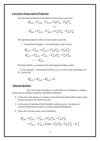
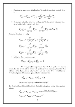
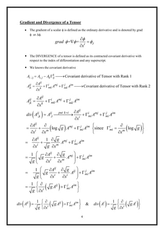
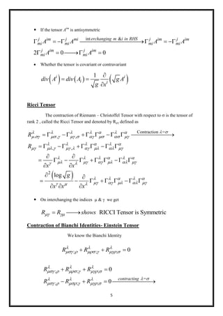
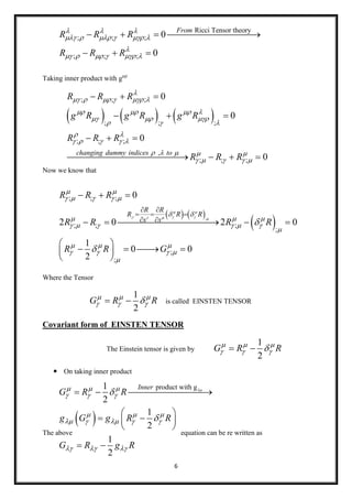
2. 2
Curvature Tensor and its Properties
We know that the Riemann Christoffel Curvature tensor is given by
Or
The important properties of this curvature tensor is given by
1. Antisymmetric property – on interchanging and  we get
This shows that R
 is antisymmetric with respect to indices and 
Cyclic property – Permuting the indices in a cyclic order and adding it can
be proved that
Bianchi Identities
Here for the sake of simplicity we shall make use of Geodesic co ordinate
system and can establish an Identity called Bianchi Identities.
 At the pole of the geodesic co ordinate system both kind of Christoffel symbol vanish,
but not necessarily their derivatives also.
 At the event of vanishing of the Christoffel symbol at a point , the process of
covariant differentiation reduces to ordinary partial differentiation
 Hence the Curvature tensor can be modified as
. , ,R      
                
. , ,
i i i i l i l
j mk jm k jk m lk jm lm jkR        
. , ,
. , ,
.
R
R
R
      
         
      
         

 
       
       
 
. . . 0R R R  
       
 
. , ,
, , since - 0
R      
         
     
       
       
       

3. 3
 The mixed curvature tensor at the Pole P0 of the geodesic co ordinate system is given
by
 On taking covariant derivative w.r.t r at the pole of the Geodesic co-ordinate system
(covariant derivative=ordinary derivative)
Permuting the indicesand 
 Adding the above equations we get
We have proved this equation at the Pole P0 of geodesic co ordinate
system. But it is in Tensor form it must hold good in every co ordinate system. Here P0 is
arbitrary point in Riemannian space but this this equation is true for all the point of the space.
Ie true for all points of Riemannian space and all co-ordinate system
This Relation is called BIANCHI IDENTITIES.
The Covariant form of Bianchi Identities is obtained by taking inner product of the equation
with g
, ,R
x x
    
       
 
      
 
2 2
; 0R at Pole P
x x x x
  
      
 
   
   
2 2
;
2 2
;
2 2
;
R
x x x x
R
x x x x
R
x x x x
  
      
  
      
  
      
 
   
   
 
   
   
 
   
   
; ; ; 0R R R  
       
; ; ; 0R R R  
       
Pr
; ; ;
; ; ;
0
0
Inner oduct g
R R R
R R R
  
     
     
   
  

4. 4
Gradient and Divergence of a Tensor
 The gradient of a scalar  is defined as the ordinary derivative and is denoted by grad
or 
 The DIVERGENCE of a tensor is defined as its contracted covariant derivative with
respect to the index of differentiation and any superscript.
 We knows the covariant derivative
,= = ii
grad
x

  

 

; j ,
;
Covariant derivative of Tensor with Rank 1
Covariant derivative of Tensor with Rank 2
k
i i j k ij
ij
ij ji mj im
mkk mkk
A A A
A
A A A
x
   

     

 
   
;
;;
log since log
ij
ij ji mj im
mkk mkk
ij
put k iij ij ji mj im
mii mik i
ij
jmj im i
mimii m m
A
A A A
x
A
div A A A A
x
A
g A A g
x x x


    


     

   
      
   
 
1
1
1
1
ij
jmj im
mii m
ij
jmj im
mii m
ij
jij im
mii i
jij im
mii
gA
A A
gx x
gA
g A A
g x x
gA
g A A
g x x
g A A
g x

   
 
 
       
 
       
 
   
 
       1 1
&jij ij im i i
mii i
div A g A A div A g A
g gx x
    
      
    

5. 5
 If the tensor Aim
is antisymmetric
 Whether the tensor is covariant or contravariant
Ricci Tensor
The contraction of Riemann – Christoffel Tensor with respect to  is the tensor of
rank 2 , called the Ricci Tensor and denoted by Rdefined as
 On interchanging the indices  we get
RICCI Tensor is SymmetricR R shows  
Contraction of Bianchi Identities- Einstein Tensor
We know the Bianchi Identity
int &
2 0 0
erchanging m i in RHSj j j jim mi im im
mi mi mi mi
j jim im
mi mi
A A A A
A A
     
   
     1i i
i i
div A div A g A
g x

 

 
Contraction =
. , ,
, ,
2
log
R
R
x x
g
x x x
       
         
     
        
     
      
    
      
          
         
 
         
 
 
        
  
; ; ; 0R R R  
       
; ; ;
=
; ; ;
0
0
contracting
R R R
R R R
  
     
   
     
  
   

6. 6
Taking inner product with g
Now we know that
Where the Tensor
1
2
G R R  
    is called EINSTEN TENSOR
Covariant form of EINSTEN TENSOR
The Einstein tensor is given by
1
2
G R R  
   
 On taking inner product
The above equation can be re written as
Ricci Tensor theory
; ; ;
; ; ;
0
0
From
R R R
R R R
  
     

     
   
  
     
; ; ;
; ; ;
; ; ;
,
; ; ;
0
0
0
0
changing dummy indices to
R R R
g R g R g R
R R R
R R R

     
   
  
  
 
    
    
    
  
  
  
   
   
 ; ;
; ; ;
; ; ;
;
;
;
0
2 0 2 0
1
0 0
2
R R
R R R
x x
R R R
R R R R
R R G
 
    
 
    
 
  
     

  
   



 
  
 
  
    
 
    
 
 
product with g1
2
1
2
1
2
Inner
G R R
g G g R R
G R g R
  
  
  
    
  


  
 
  
 
 

7. 7
 Divergence of Einstein tensor- According to the definition of divergence of a tensor
   ;Sin 0
; 0
ce G
div G G div G

   
   

  
GEODESICS
 In Euclidean 3D space ( Flat space ) the path of shortest distance between two fixed
points is a straight line. But in Riemannian space (Non-Euclidean space ) the Path of
extremum ( Maximum or minimum) distance between any two points in Riemannian
space is called GEODESIC
 Thus it is determined by the condition that , the path between any two fixed points A
and b is given by
 In Riemannian space we have
 Keeping end points fixed path of the trajectory is deformed giving an arbitrary
infinitesimal displacement xm
,
On differentiating above equation
1
2
G R g R   
We can write
extremum ( or stationery ) 0
B B
Hence
A A
ds ds   
2 i j
ijds g dx dx
       
   
   
2
by 2ds
On differentiating
2
1
2
i j
ij
i j i j i j
ij ij ij
iji j m j i i j
ij ijm
i j j i
ijDividing m i
ij ijm
ds g dx dx
ds ds g dx dx g dx dx g dx dx
g
dx dx x g dx dx g dx dx
x
gdx dx dx d dx d
ds x g x g
ds ds ds ds ds dx
   
  
  

  

  


   

 
 
   
since 0 &
1
0
2
j
B i
i
A
B i j j i
ij m i j
ij ijm
A
x ds
s
dx d
ds x
ds ds
gdx dx dx d dx d
x g x g x ds
ds ds ds ds ds dsx

  
  
  
 
  
  
    
   
  
    
  



8. 8
   
 
 
1
0
2
1
0
2
1
2
B i j j i
ij m m m
mj imm
A
B i j j i
ij m m
mj imm
A
i j j i
ij m m
mj imm
gdx dx dx d dx d
x g x g x ds
ds ds ds ds ds dsx
gdx dx dx dx d
x g g x ds
ds ds ds ds dsx
gdx dx dx dx d
x g g x
ds ds ds ds dsx
  
 
 
  
    
  
   
         
  
      


 
0
On Integrating the II term
1 1
= 0
2 2
B
A
B Bi j j i
ij m m
mj imm
A A
ds
gdx dx dx dx d
x ds g g x ds
ds ds ds ds dsx
 
 
 
  
    
              

 
As the infinitesimal displacement xm
, is arbitrary, the integrand must vanish . Ie term inside
the bracket must be zero
Hence we can write
i j j i
ij
mj imm
gdx dx d dx dx
g g
ds ds ds ds dsx
 
     
1 1
= 0
2 2
BB Bi j j i j i
ij m m m
mj im mj imm
A AA
gdx dx dx dx d dx dx
x ds g g x g g x ds
ds ds ds ds ds ds dsx
  
      
                       
 
1
0
2
B i j j i
ij m
mj imm
A
gdx dx d dx dx
g g x ds
ds ds ds ds dsx

   
         

i j j i
ij
mj imm
gdx dx d dx dx
g g
ds ds ds ds dsx
 
     
2 2
2 2
2 2
2 2
i j j j i i
ij mj im
mj imm
i j i j j j i i
ij mj im
mj imm i j
g dg dgdx dx dx d x dx d x
g g
ds ds ds ds ds dsx ds ds
g dg dgdx dx dx dx d x dx dx d x
g g
ds ds ds ds ds dsx dx ds dx ds

   


   


9. 9
 
2 2
2 2
2 2
2 2
Replace &
i j i j j i i j
ij mj im
im mjm i j
i j l l
ij mj im
lm mlm i j
g dg dgdx dx dx dx dx dx d x d x
g g
ds ds ds ds ds dsx dx dx ds ds
g dg dgdx dx d x d x
g g i j by l
ds ds x dx dx ds ds

   

 
     
 
2
2
2
2
2
2
i j l
ij mj im
lmm i j
i j l
ij mj im
lmm i j
g dg dgdx dx d x
g
ds ds x dx dx ds
g dg dgdx dx d x
g
ds ds x dx dx ds
 
   
 
 
     
 
2
2
1
2
i j l
ij mj im
lmm i j
g dg dgdx dx d x
g
ds ds x dx dx ds
  
      
   
 Taking inner product with gmp
2
2
1
2
i j l
jm ijpm mpim
lmj i m
dg gdgdx dx d x
g g g
ds ds dx dx x ds
  
     
   
2
2
2
2
2
2
0
0
i j l
p p
ij l
i j p
p
ij
k i j
k
ij
dx dx d x
ds ds ds
dx dx d x
ds ds ds
d x dx dx
ds dsds

 
   
  
  
  
 This equation represents the differential equation of a GEODESIC. For k=1,2,3,4 this
equation gives four differential equation which determine a GEODESIC
2
2
0
k i j
k
ij
d x dx dx
ds dsds
  

10. 10
NEWTON’S EQUATION OF MOTION AS AN APPROXIMATION OF
GEODESIC EQUATIONS
Let us consider the motion of a test particle in a very weak static field, so that its velocity is
non- Relativistic. The Geodesic equation of motion of the test particle in a curved space
geometry is
For a flat space , the Christoffel symbol vanishes , and in that case Geodesic equation reduce
the equations of Straight lines.
The metric tensor gdetermines both the line element and the equations of the motion.First
case it determines the structure of the geometry while in the second case Christoffel symbol (
derivative of metric tensor) determine the trajectory of the test particle.
 Comparing the equations of motion with Newton’s equations of motion we conclude
that gplay the role of Gravitational potential 
 Let us establish a connection between Geodesic equation of motion with the Newton’s
equation of motion
The component of a metric tensor g in Euclidean space denoted by are all constants given
by 
 Since
2
2
0
d x dx dx
ds dsds
  

  
2
2
0
d x
ds


2
4 G   
1 0 0 0
0 1 0 0
0 0 1 0
0 0 0 1
g 
 
 
  
 
 
 
2
2 2 2 2 2
Riemannian Space
Euclidean Space
ds g dx dx
dx dy dz c dt In
 
 
     

11. 11
Let us now assume that are not constants , but differ from above values by an infinitesimal
amount in a weak magnetic field. In weak B no relativistic condition to be applied
4
0
, ,
1
2
1
2
v v
v v
where are small quantities and functions
g
of x y z but independent of time c tx
g g g
g
x x x
x x x
 
  
   
   
   
  
 
 
  
 
  
    
 
   
    
   
   
          
1
since
2
vv
x x x x x
   
    
   

    
    
     
In Galilean co ordinates
Then we get
By virtue of above equation
From above equations
1 2 3 4
2 2 2 2 2 2
, , ,x x x y x z and x ct
we get ds dx dy dz c dt
   
    
1 2 3 4
0 & 1
dx dx dx dx
ds ds ds ds
   
1 2 3 4
2 2 2 2 2 2
2
2 2 2 2 2 2 2 2 2
2 4
, , ,
1
0,
x x x y x z and x ct
we get ds dx dy dz c dt
for small velocities v cv
ds v dt c dt c dt c dt
c v c ds cdt dx
   
    
    
        
        
2
2
22 4
2
2 2
4, 4
442 2
0
0
0 0
d x dx dx
ds dsds
d x dx
dsds
d x d x
ds ds
  





 
  

 
  
 
   
  
      

12. 12
2 2
44 442 2
1,2,34 4 44 44
444 4
2 2
244
44 44 442 2
2
tons Eqn= Geodesi
2
0 0
1 1
2 2
1 1
0
2 2
New
d x d x
ds ds
x x x x
d x d x
c g
ds ds x x
d x
ds x
 
 
  
  
 
 
 


   



      
      
          
      
    
          
   

 

2
c Eqn 2
442
2
44
1
2
1
2
d x
c g
ds x
c g
x x


 

  
    
 
  
   
  
On integrating
Integrating44
442 2
2 2Ong
dx dx g k
x c x c
 
 
  
   
 
 
Since in flat space g44=1 and =0 so that k=1
Hence the geodesic equation are reducible to Newton’s equations of motion in the case of a
weak magnetic field if
2 2
tons Eqn= Geodesic Eqn 2
442 2
1
2
Newd x d x
c g
ds x ds x
 
 
   
      
  
When RHS of the equation become
2
2 2
44 2
1 1 2
1
2 2 2
c
c g c
x x c x x   
 

       
             
          
Newton’s theory of gravitation can be regarded as giving first approximation to the general
theory of relativity with quantity g44 of the General theory closely related to the Gravitational
Potential  of the Newton theory
Sin 1
44 442 2
2 2
1
ce k
g k g
c c
 
    
44 2
2
1g
c

 

13. 13
Therefore we can assume the GRAVITATIONAL FIELD is represented by the metric
tensor (g) and the equations of motion of the particle in a Gravitational field are given by
GEODESIS EQUATION OF MOTION
Material Energy Tensor
If 0 is the proper density of matter and refers to the motion of the
Matter, then in relativistic unit the material energy tensor is defined as
If is the co ordinate density of matter moving with velocity v relative to Galilean co
ordinates then
0 0
2 2 2
2 2 2 2 2
2 2 2 2
2
2
0 0
02 2 2
= in relativistic units
1 1
Hence 1 1
1 1
v c v
In Galilean co ordinates ds dx dy dz dt
ds dx dy dz
v
dt dt dt dt
ds
dtv c v
 

 
  
 
 
     
       
             
       
 
     
   
 Hence Galilean co ordinate equation becomes
2
0
2
0
ds
dtdx dx ds dx dx
T T
ds ds dt ds ds
dx ds dx ds dx dx
T T
ds dt ds dt dt dt
    
 
   
 
 
 
 
  
   
    
 
   
     
   
 Considering u,v,w as the components of velocity then we have
Then we get in Matrix form as
dx
ds

0
dx dx
T
ds ds
 


1 2 3 4
1,2,3,4
v 1
dx dx dx dx dx
u or or w or
dt dt dt dt dt

           
                    

14. 14
11 12 13 14 2
21 22 23 24
31 32 33 34
41 42 43 44
T T T T u uv uw u
T T T T uv
T
T T T T
T T T T

   

 
 
 
  
 
 
 
2
2
v vw v
uw vw w w
u v w
  
   
   
 
 
 
 
 
 
 
In automatically constituted matter a volume which is regarded as small macroscopic
treatment contains particles with widely varying motions . Thus above matrix elements must
be summed up for varying motion of the particle . Hence we must add tensor formed by the
internal stresses
 
2
2
2
T , , ,
xx xy xz
yx yy yz
zx zy zz
x y z
p u p uv p uw u
p uv p v p vw v
T
p uw p vw p w w
u v w


 
   
   
   
  

  
  

  
Re
, ,
present the whole density
u v w mass motion of the macroscopic element


 
 
 
 
 
 
  


Let us consider a relation
     
4
0
Taking first then
u v w
x y z t
which represents the Equation of continuity in Hydrodynamics

   

   
   
   
       
2
1
0
xyxx xz
Taking then
up uv uw up p
x y z x y z t

   

    
      
      
0
1,2,3,4
case study can be done byT
puttingx

 
 
  
  

15. 15
       
       
 
2
Taking u as first term and u/ v/ w/ as second term on differ.
0
xyxx xz
up uv uw up p
x y z x y z t
u v w u u u u
u u v w
x y z t x y z t
u u
u u v w
x y
   
   
   


             
       
 
         
                    
  
    
 
u u u u u u
u v w
z t x y z t
du d
where u v w
dt dt x y z t


       
                
    
      
    
Similarly we can obtain
1
2
3
xy Putxx xz
yx yy yz Put
zy Putzx zz
pp p du
x y z dt
p p p dv
x y z dt
pp p dw
x y z dt









 
    
  
  
    
  
 
    
  
Here , & represent the components of the
accelaration of the element of the fluid
du dv dw
dt dt dt
The above equations express directly the conservation of mass and momentum so that in
Galilean co ordinates the principles of conservation of mass and momentum are contained
As 
 relative to Galilean co ordinates, Hence
 
 
Covariant derivative reduce to Ordinary derivative
;
;
0 0 ivergence of 0
T
T
x
T
Hence T D T
x




 
 

 


    


16. 16
Hence
var
As represent the rate of creation of mass and momentum in unit volume
It is often convenient to use mixed tensor T in place of contra iant ten or T
T
x
s







Then T g T 
 