Content
1. Two Typesof Random Variables
2. Probability Distributions for Discrete
Random Variables
3. The Binomial Distribution
4. Poisson and Hypergeometric Distributions
5. Probability Distributions for Continuous
Random Variables
6. The Normal Distribution
3.
Content (continued)
7. DescriptiveMethods for Assessing
Normality
8. Approximating a Binomial Distribution
with a Normal Distribution
9. Uniform and Exponential Distributions
10. Sampling Distributions
11. The Sampling Distribution of a Sample
Mean and the Central Limit Theorem
4.
Learning Objectives
1. Developthe notion of a random variable
2. Learn that numerical data are observed values of
either discrete or continuous random variables
3. Study two important types of random variables
and their probability models: the binomial and
normal model
4. Define a sampling distribution as the probability of
a sample statistic
5. Learn that the sampling distribution of follows a
normal model
x
5.
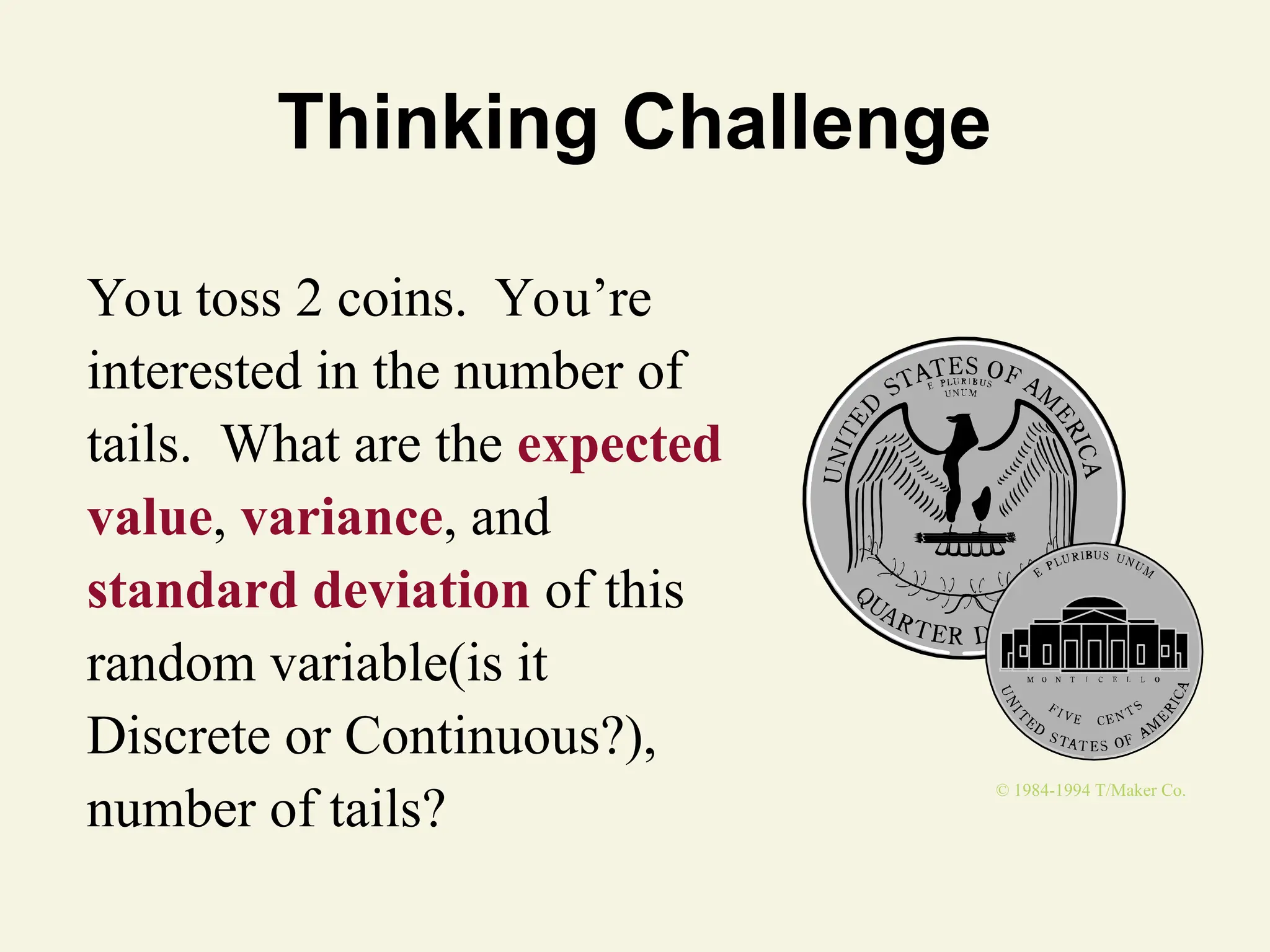
Thinking Challenge
• You’retaking a 33 question
multiple choice test. Each
question has 4 choices. Clueless
on 1 question, you decide to
guess. What’s the chance you’ll
get it right?
• If you guessed on all 33
questions, what would be your
grade? Would you pass?
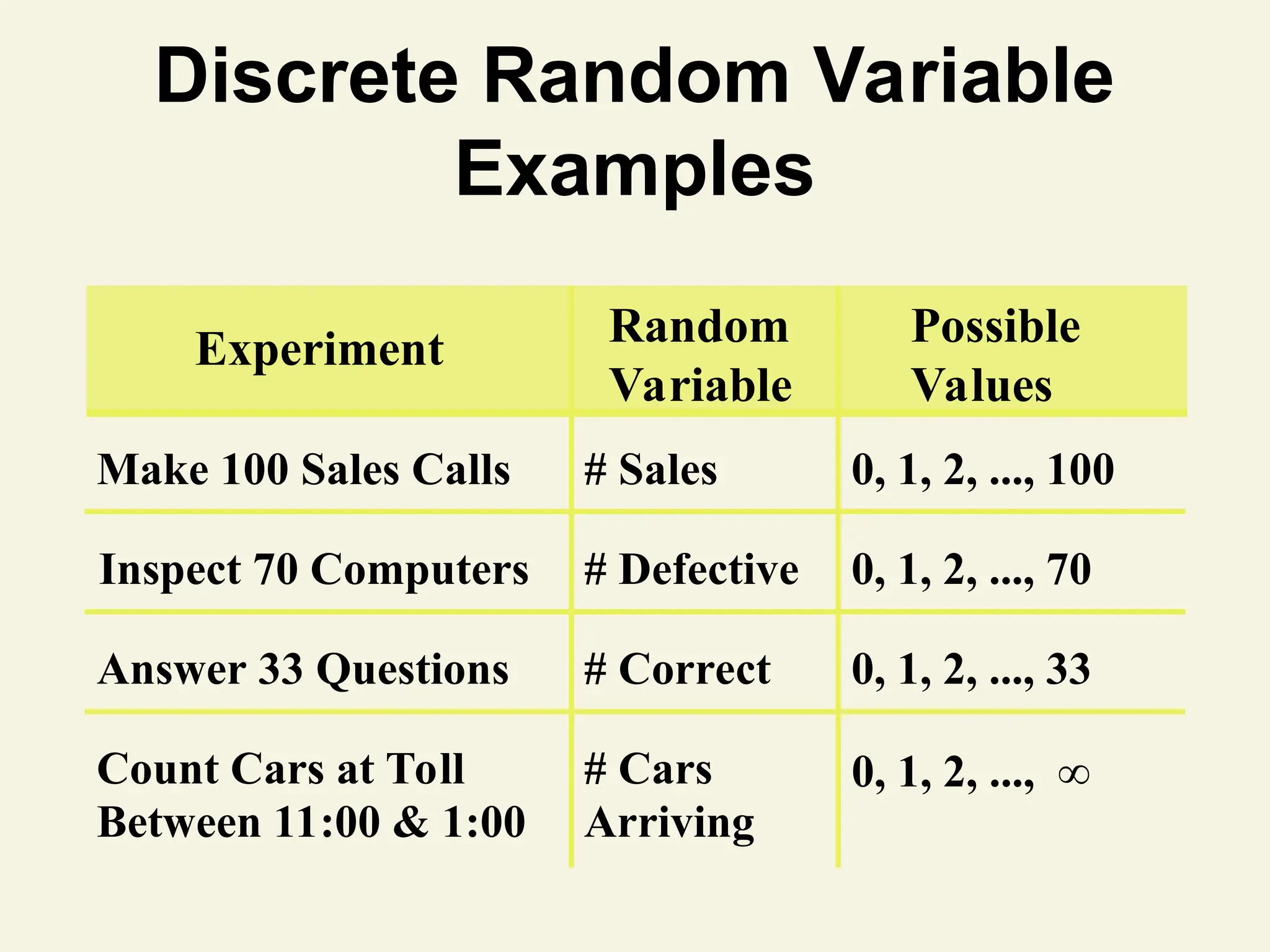
Random Variable
A randomvariable is a variable that assumes
numerical values associated with the random
outcomes of an experiment, where one (and only
one) numerical value is assigned to each sample
point.
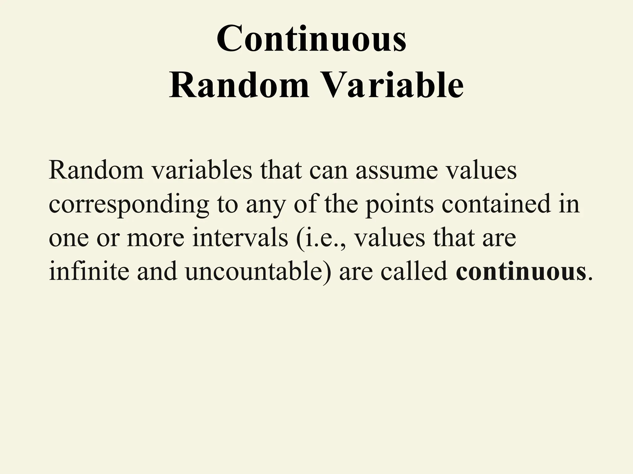
Continuous
Random Variable
Random variablesthat can assume values
corresponding to any of the points contained in
one or more intervals (i.e., values that are
infinite and uncountable) are called continuous.
11.
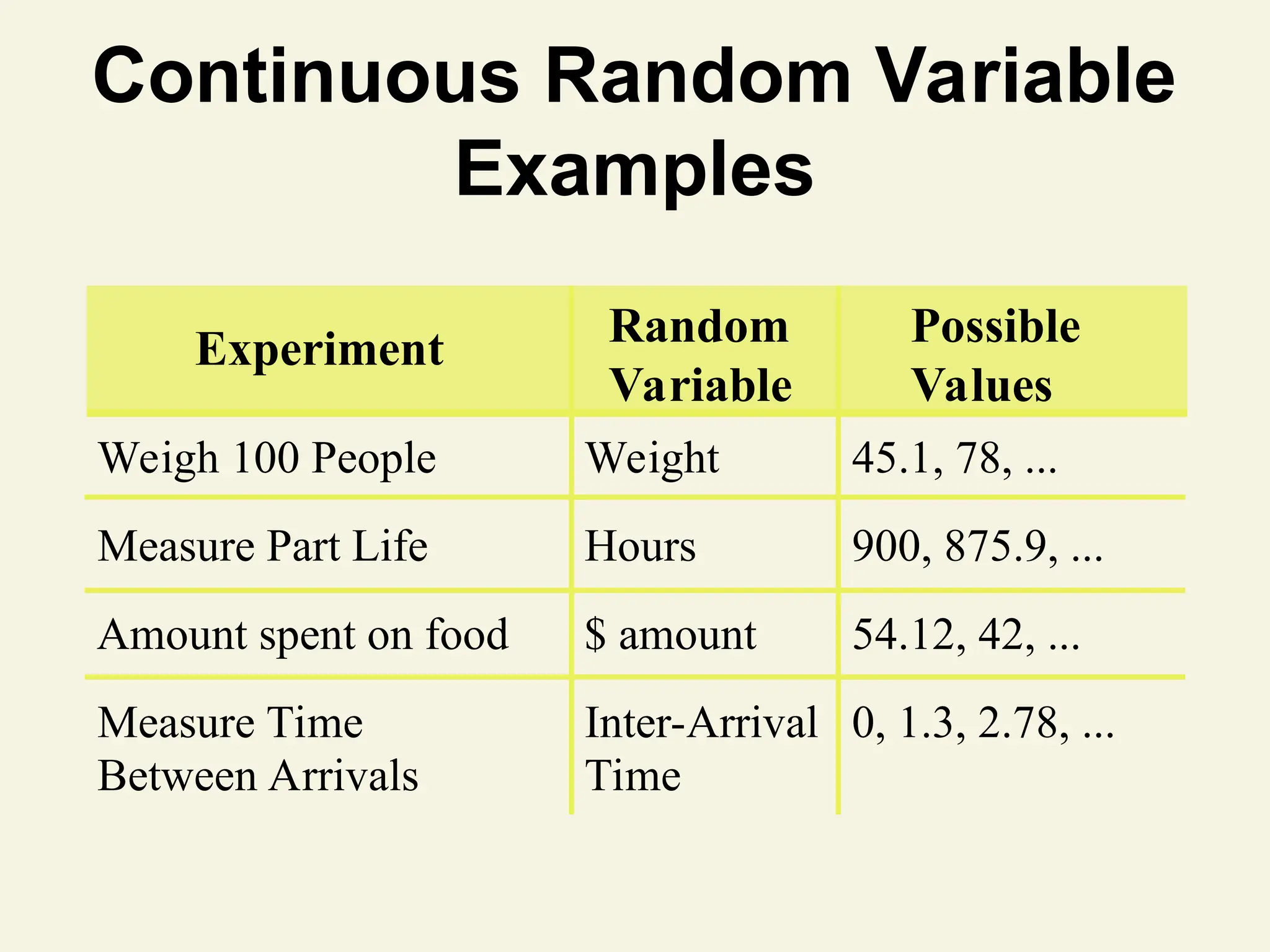
Continuous Random Variable
Examples
MeasureTime
Between Arrivals
Inter-Arrival
Time
0, 1.3, 2.78, ...
Experiment Random
Variable
Possible
Values
Weigh 100 People Weight 45.1, 78, ...
Measure Part Life Hours 900, 875.9, ...
Amount spent on food $ amount 54.12, 42, ...
Discrete
Probability Distribution
The probabilitydistribution of a discrete
random variable is a graph, table, or formula
that specifies the probability associated with each
possible value the random variable can assume.
14.
Requirements for the
ProbabilityDistribution of a
Discrete Random Variable x
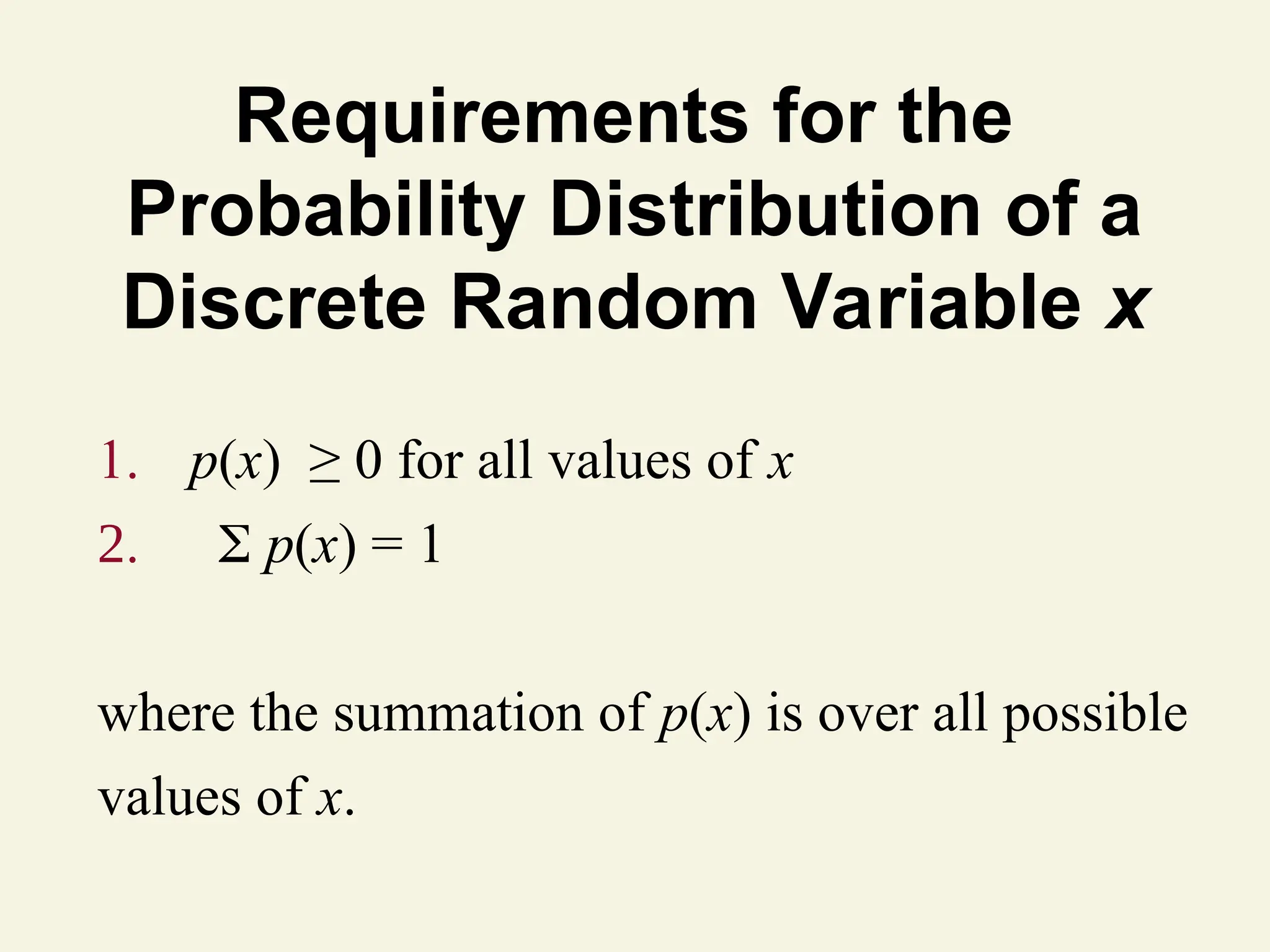
1. p(x) ≥ 0 for all values of x
2. p(x) = 1
where the summation of p(x) is over all possible
values of x.
Visualizing Discrete
Probability Distributions
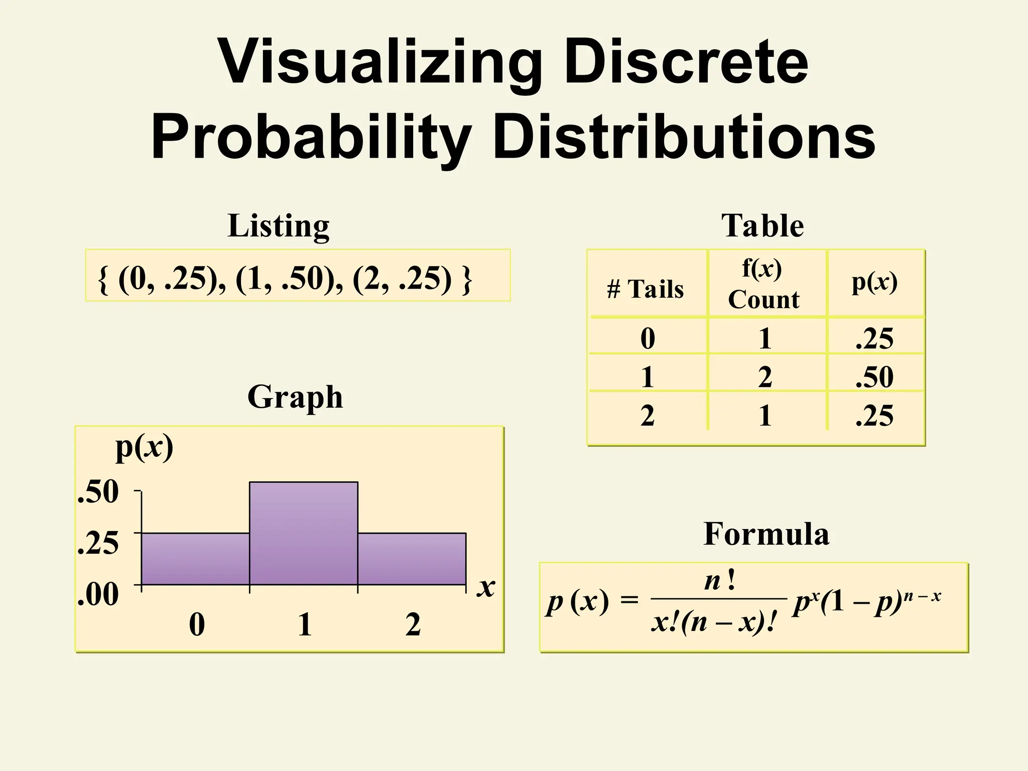
ListingTable
Formula
# Tails
f(x)
Count
p(x)
0 1 .25
1 2 .50
2 1 .25
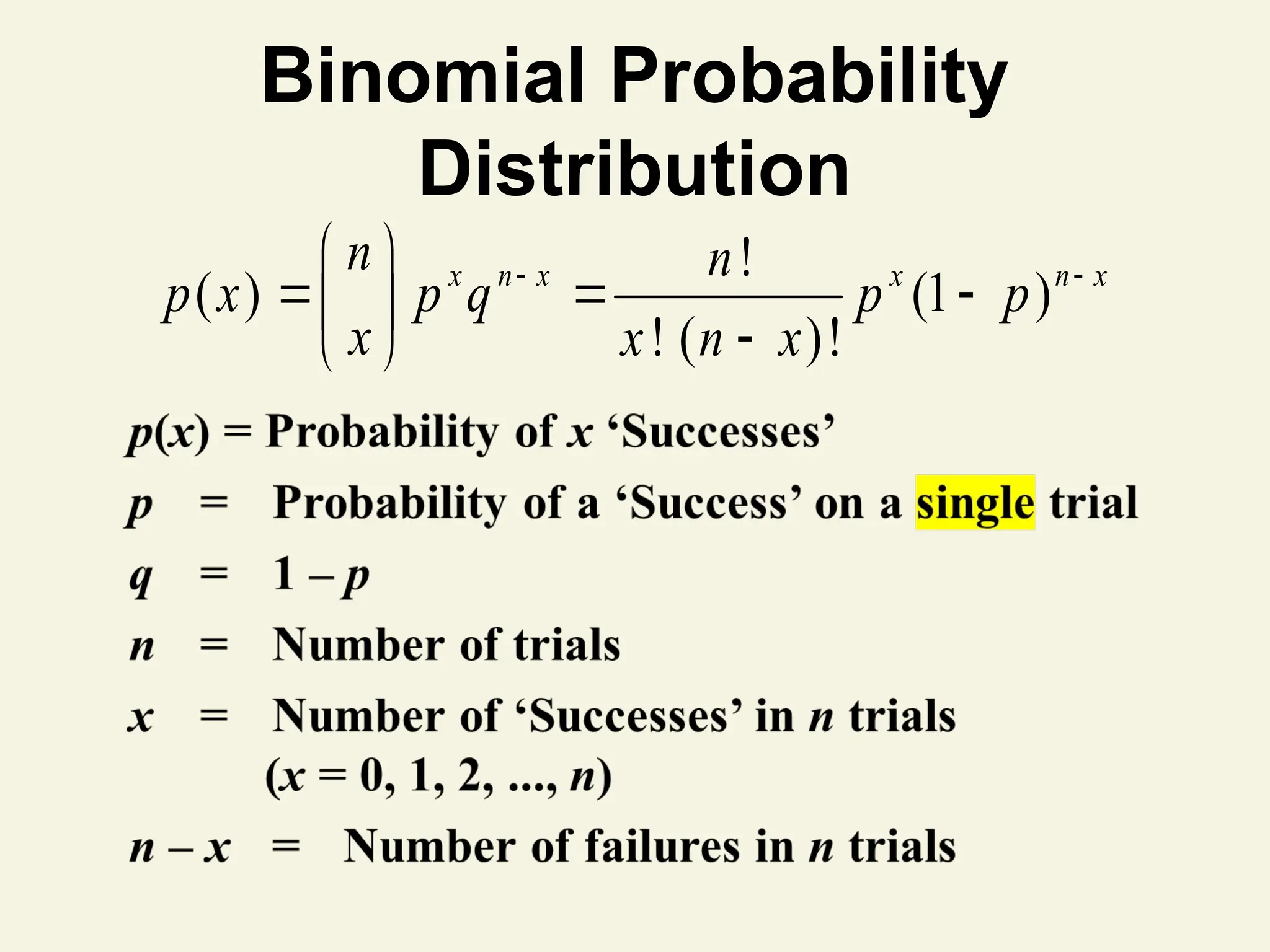
p x
n
x!(n – x)!
( )
!
= px
(1 – p)n – x
Graph
.00
.25
.50
0 1 2
x
p(x)
{ (0, .25), (1, .50), (2, .25) }
17.
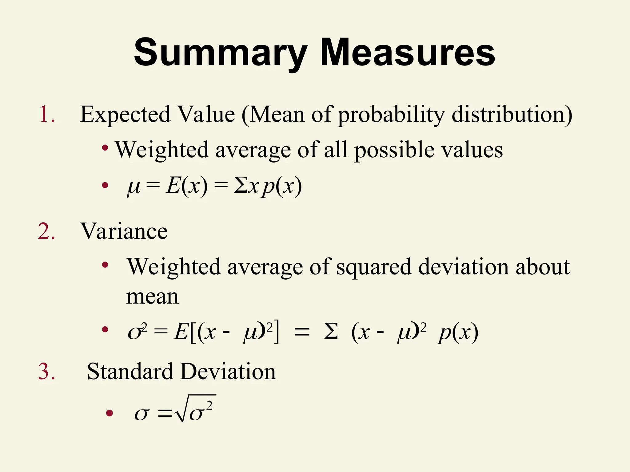
Summary Measures
1. ExpectedValue (Mean of probability distribution)
• Weighted average of all possible values
• = E(x) = xp(x)
2. Variance
• Weighted average of squared deviation about
mean
• 2
= E[(x
(x
p(x)
3. Standard Deviation
2
●
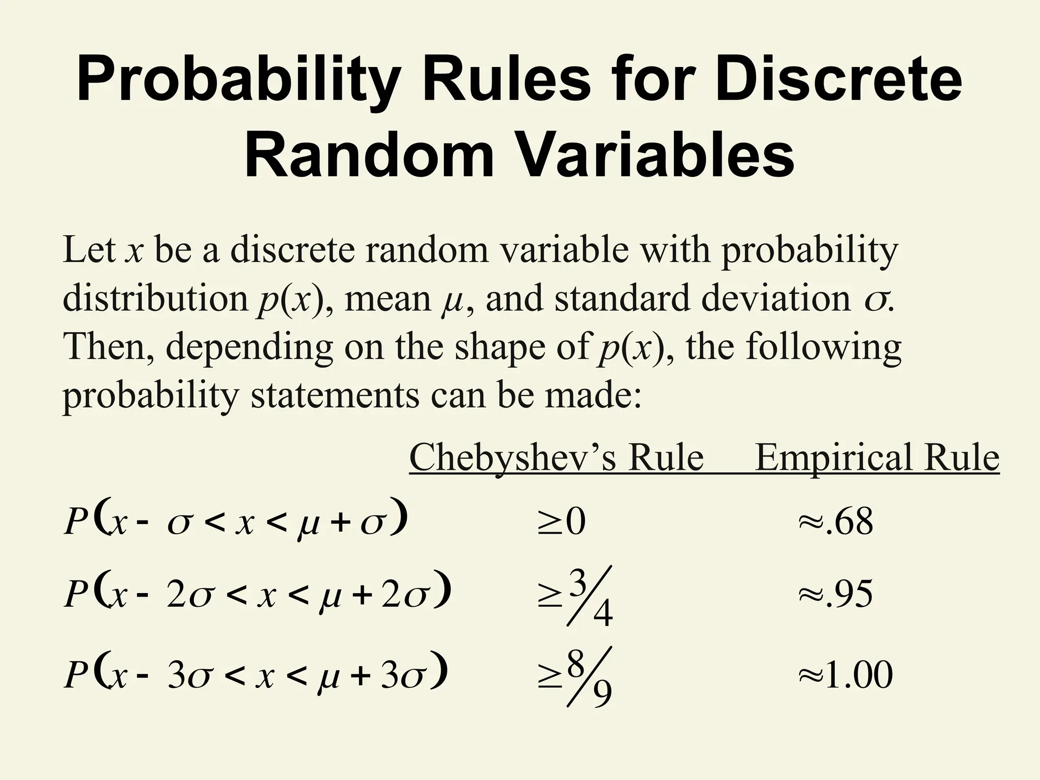
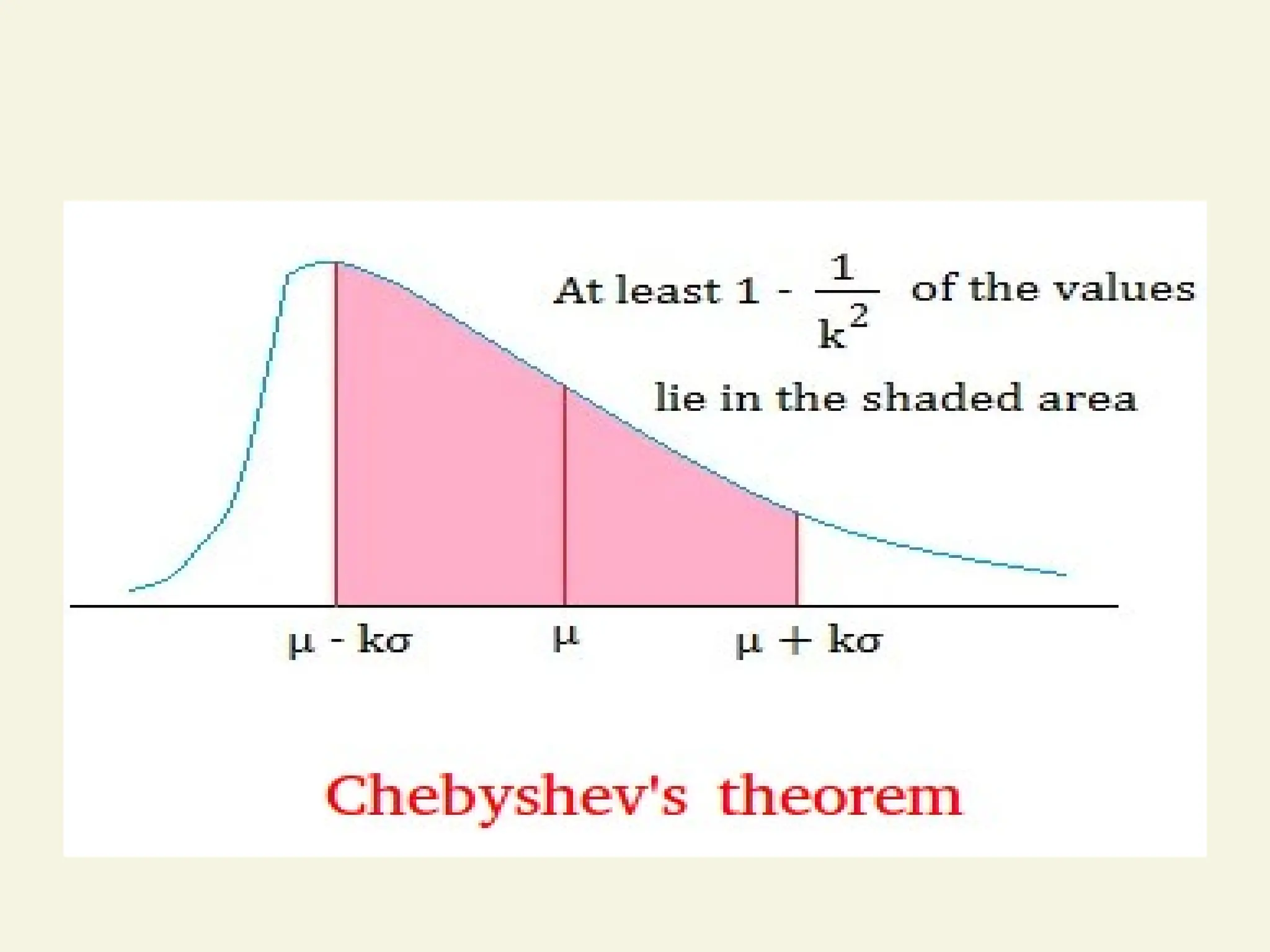
Probability Rules forDiscrete
Random Variables
Let x be a discrete random variable with probability
distribution p(x), mean µ, and standard deviation .
Then, depending on the shape of p(x), the following
probability statements can be made:
Chebyshev’s Rule Empirical Rule
P x x µ
0 .68
P x 2 x µ 2
3
4 .95
P x 3 x µ 3
8
9 1.00
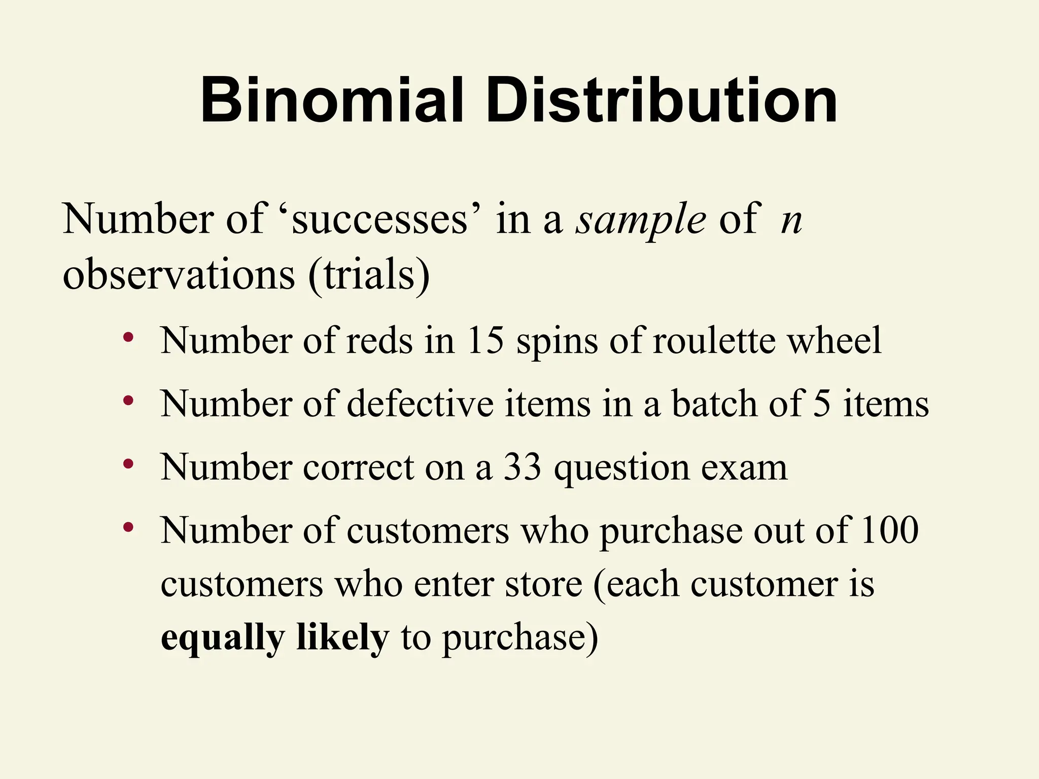
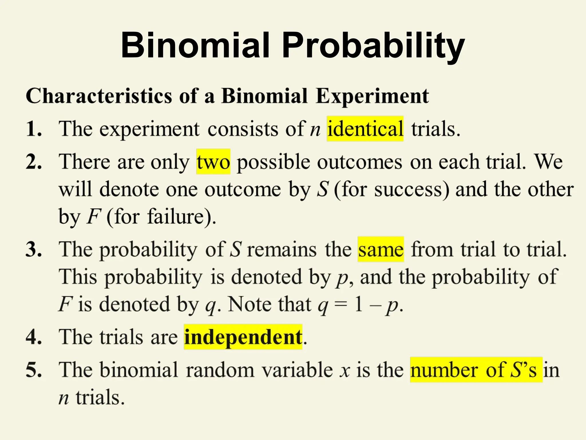
Binomial Distribution
Number of‘successes’ in a sample of n
observations (trials)
• Number of reds in 15 spins of roulette wheel
• Number of defective items in a batch of 5 items
• Number correct on a 33 question exam
• Number of customers who purchase out of 100
customers who enter store (each customer is
equally likely to purchase)
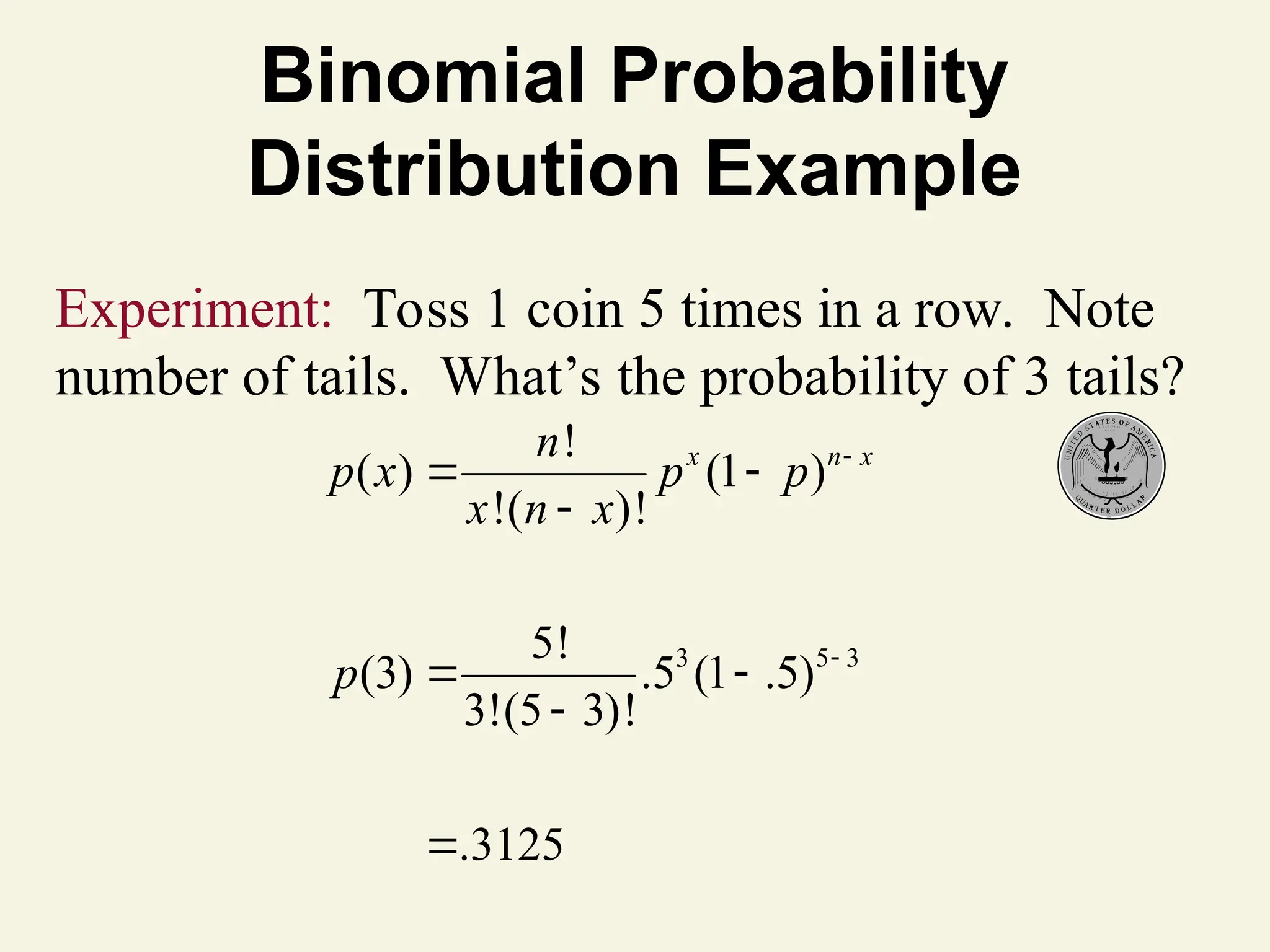
Binomial Probability
Distribution Example
35 3
!
( ) (1 )
!( )!
5!
(3) .5 (1 .5)
3!(5 3)!
.3125
x n x
n
p x p p
x n x
p
Experiment: Toss 1 coin 5 times in a row. Note
number of tails. What’s the probability of 3 tails?
Binomial Distribution
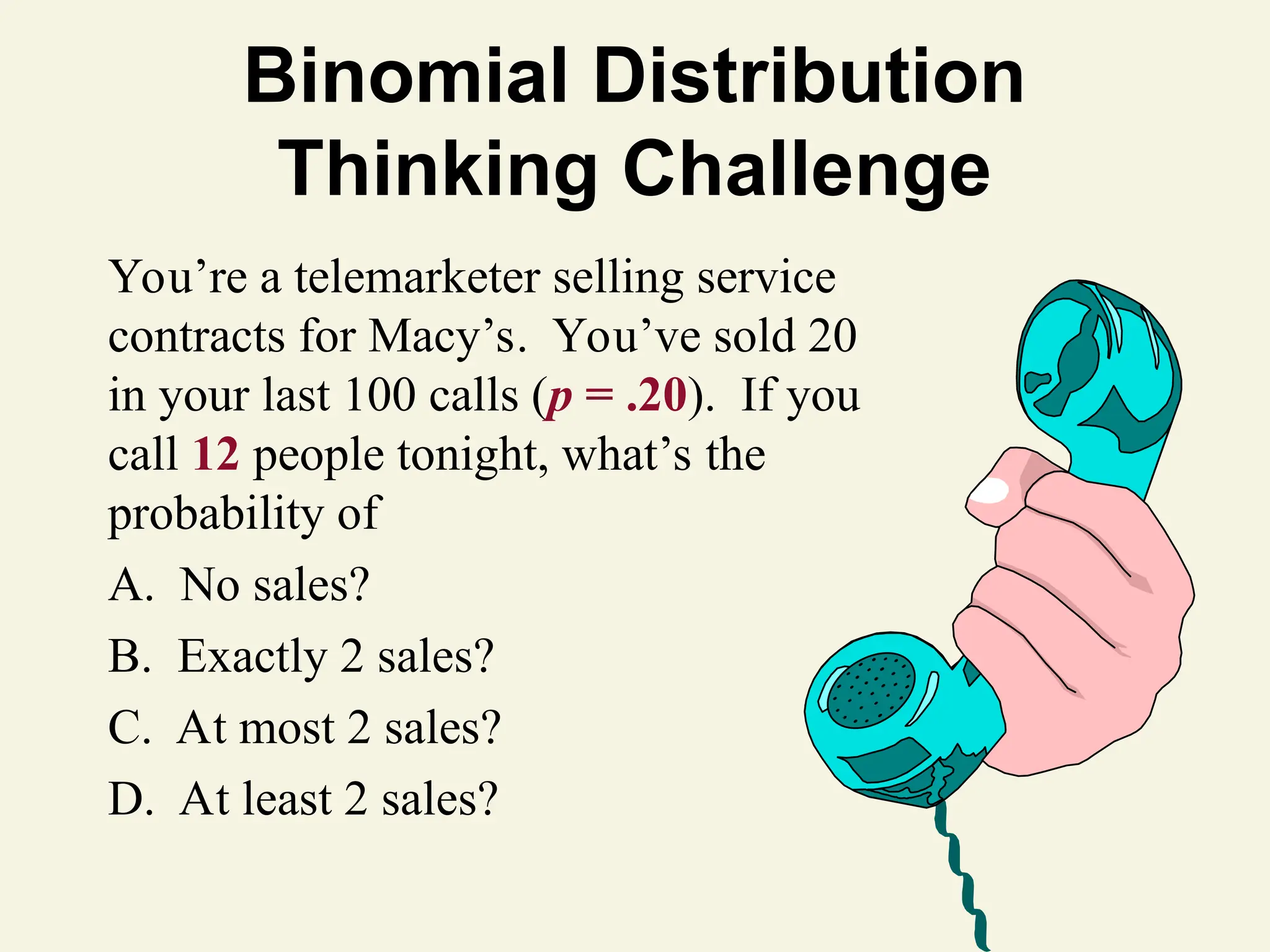
Thinking Challenge
You’rea telemarketer selling service
contracts for Macy’s. You’ve sold 20
in your last 100 calls (p = .20). If you
call 12 people tonight, what’s the
probability of
A. No sales?
B. Exactly 2 sales?
C. At most 2 sales?
D. At least 2 sales?
33.
Binomial Distribution Solution*
n= 12, p = .20
A. p(0) = .0687
B. p(2) = .2835
C. p(at most 2) = p(0) + p(1) + p(2)
= .0687 + .2062 + .2835
= .5584
D. p(at least 2) = p(2) + p(3)...+ p(12)
= 1 – [p(0) + p(1)]
= 1 – .0687 – .2062
= .7251
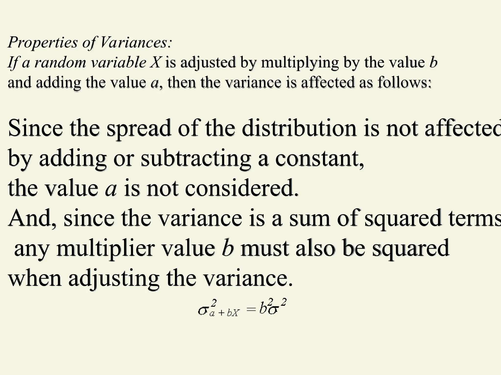
Properties of Variances:
Ifa random variable X is adjusted by multiplying by the value b
and adding the value a, then the variance is affected as follows:
Since the spread of the distribution is not affected
by adding or subtracting a constant,
the value a is not considered.
And, since the variance is a sum of squared terms
any multiplier value b must also be squared
when adjusting the variance.
36.
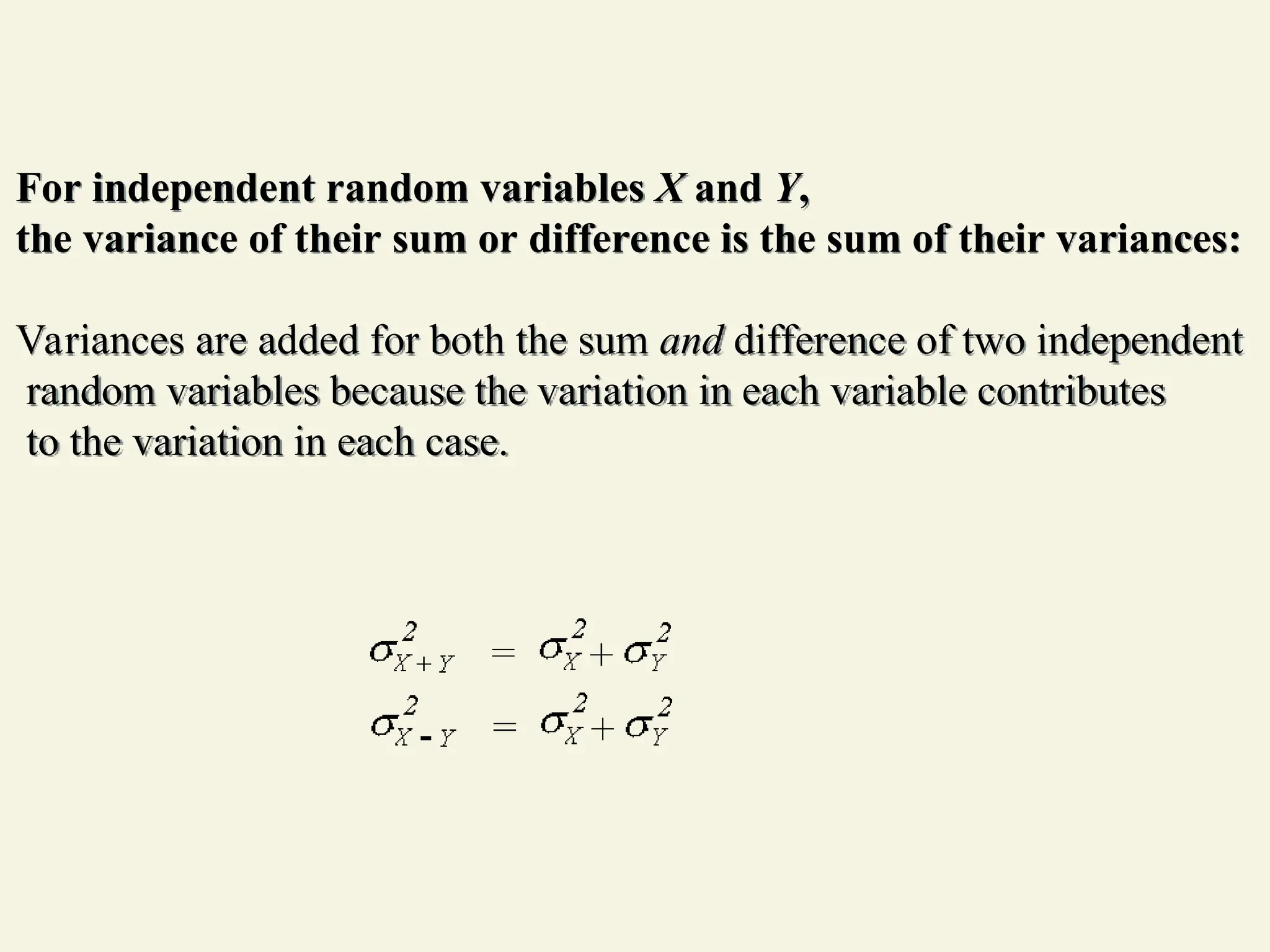
For independent randomvariables X and Y,
the variance of their sum or difference is the sum of their variances:
Variances are added for both the sum and difference of two independent
random variables because the variation in each variable contributes
to the variation in each case.
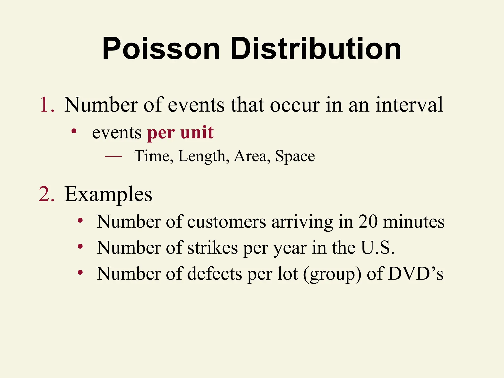
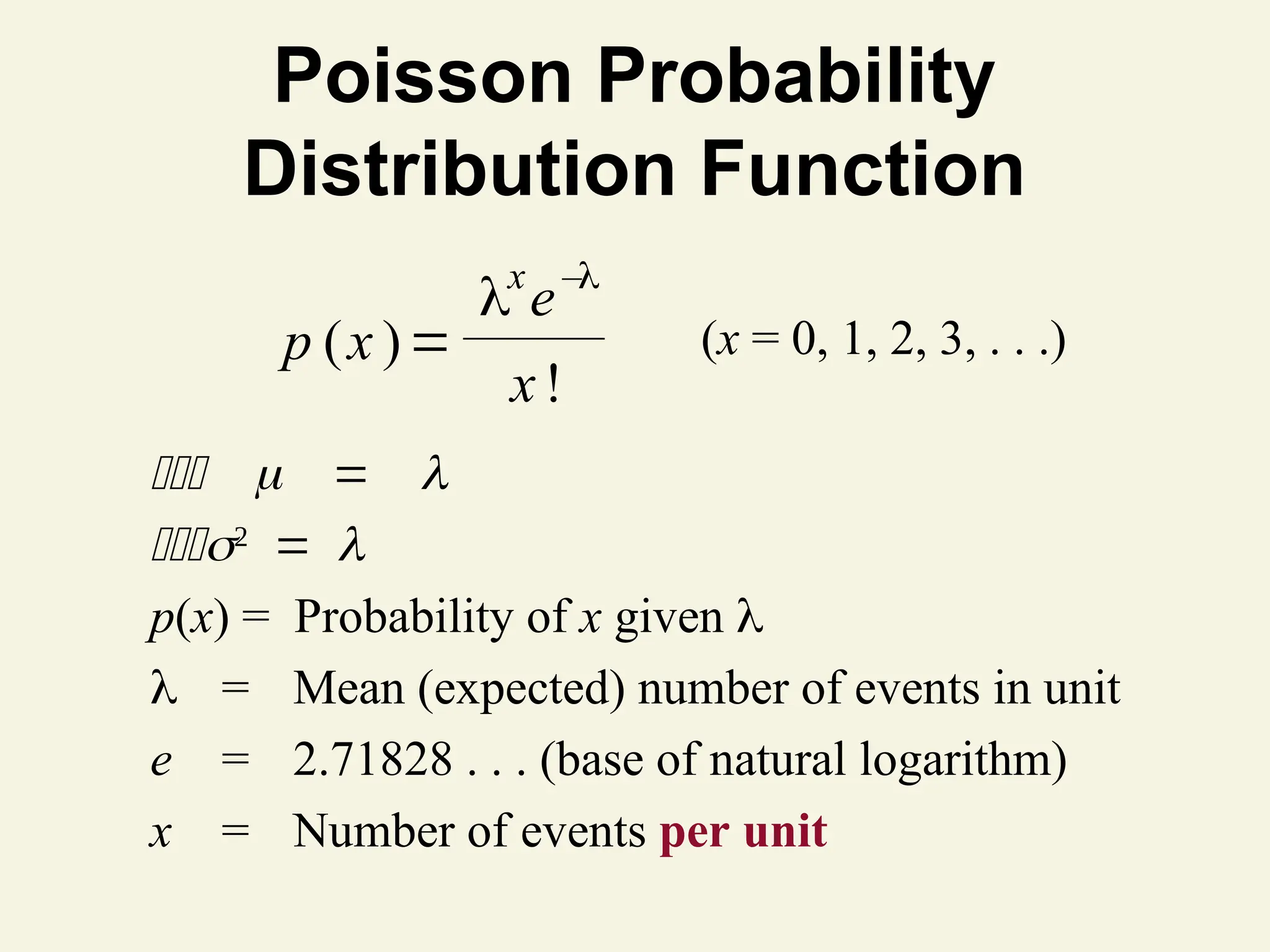
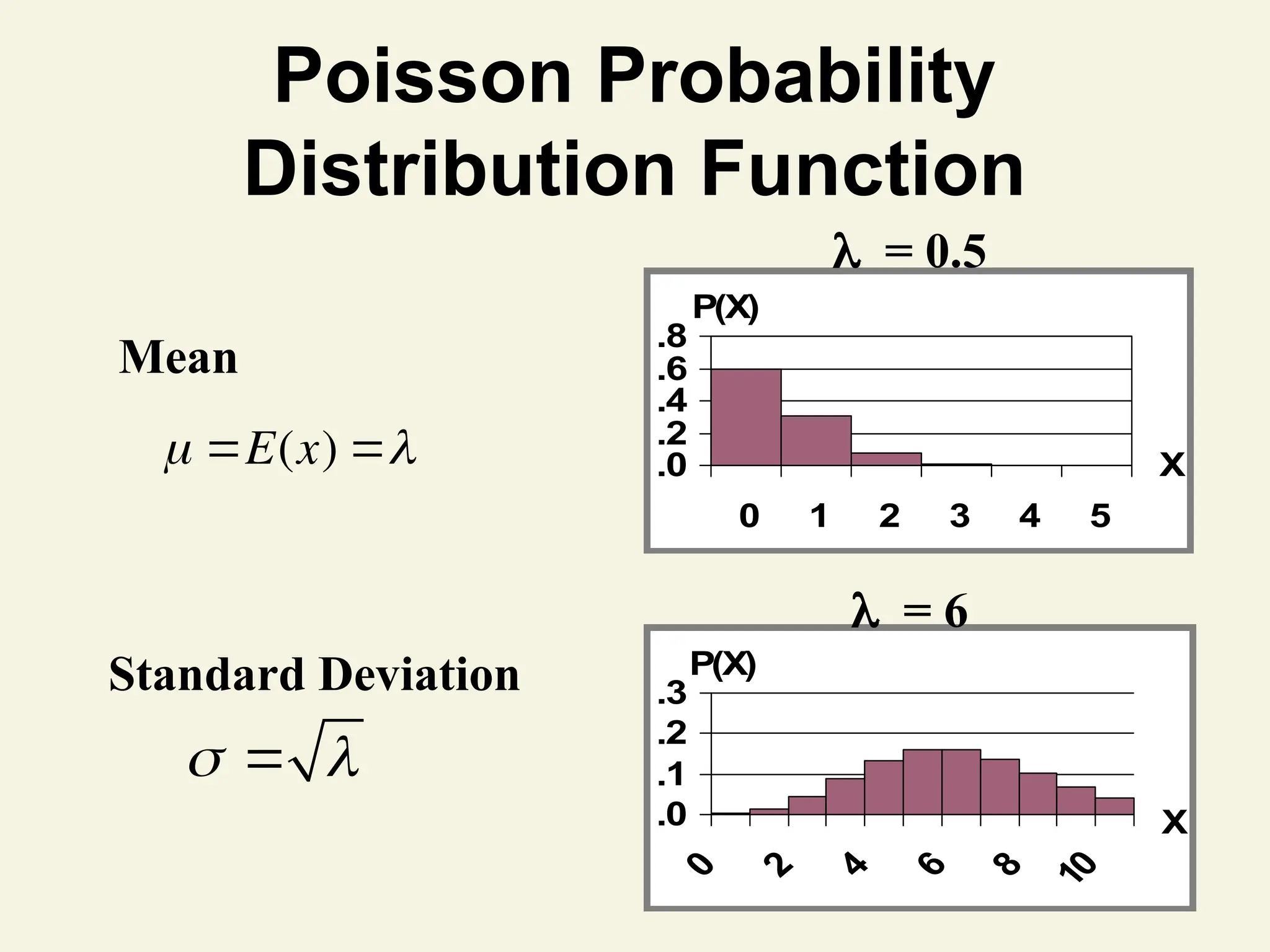
Poisson Distribution
1. Numberof events that occur in an interval
• events per unit
— Time, Length, Area, Space
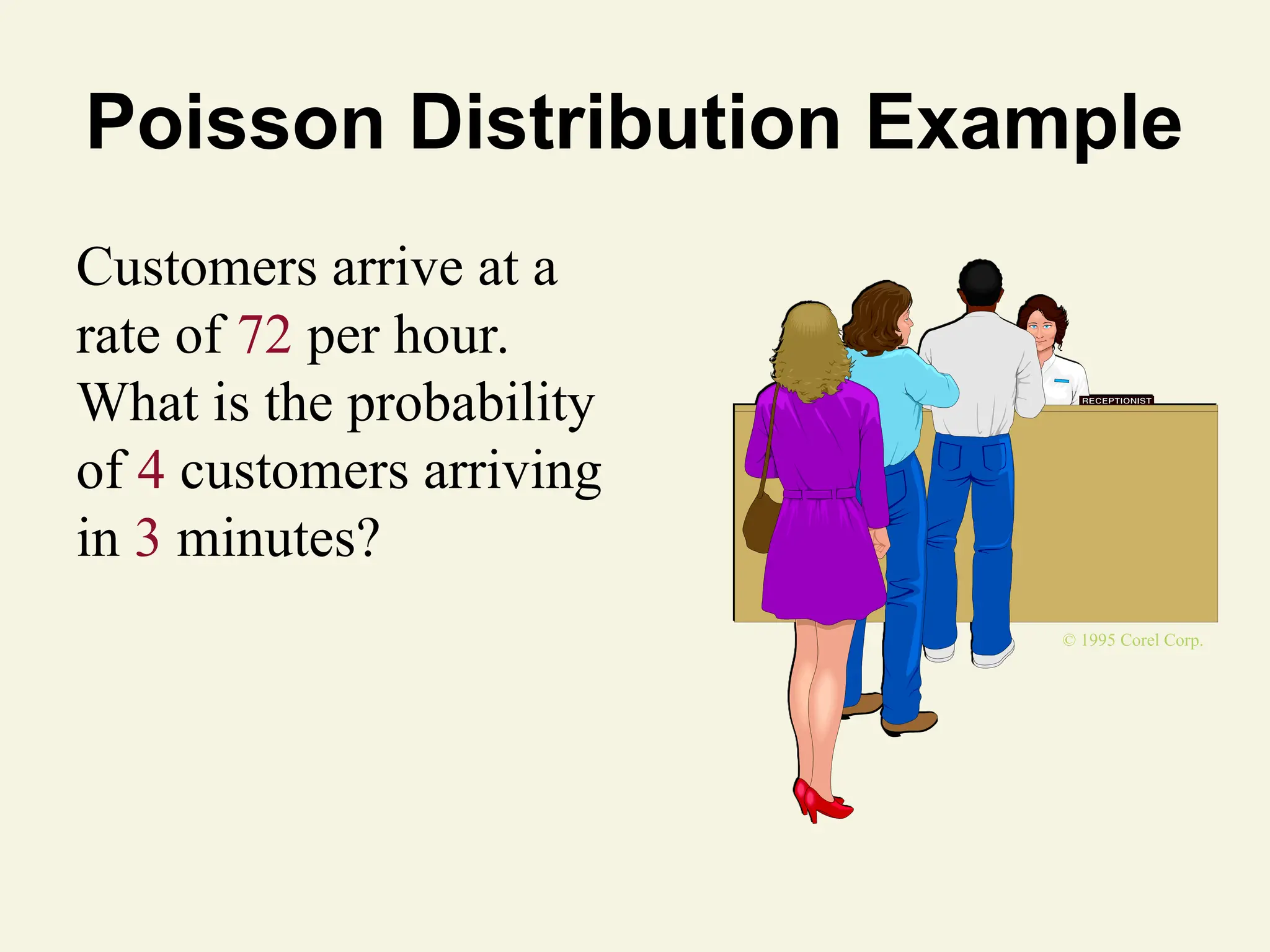
2. Examples
• Number of customers arriving in 20 minutes
• Number of strikes per year in the U.S.
• Number of defects per lot (group) of DVD’s
39.
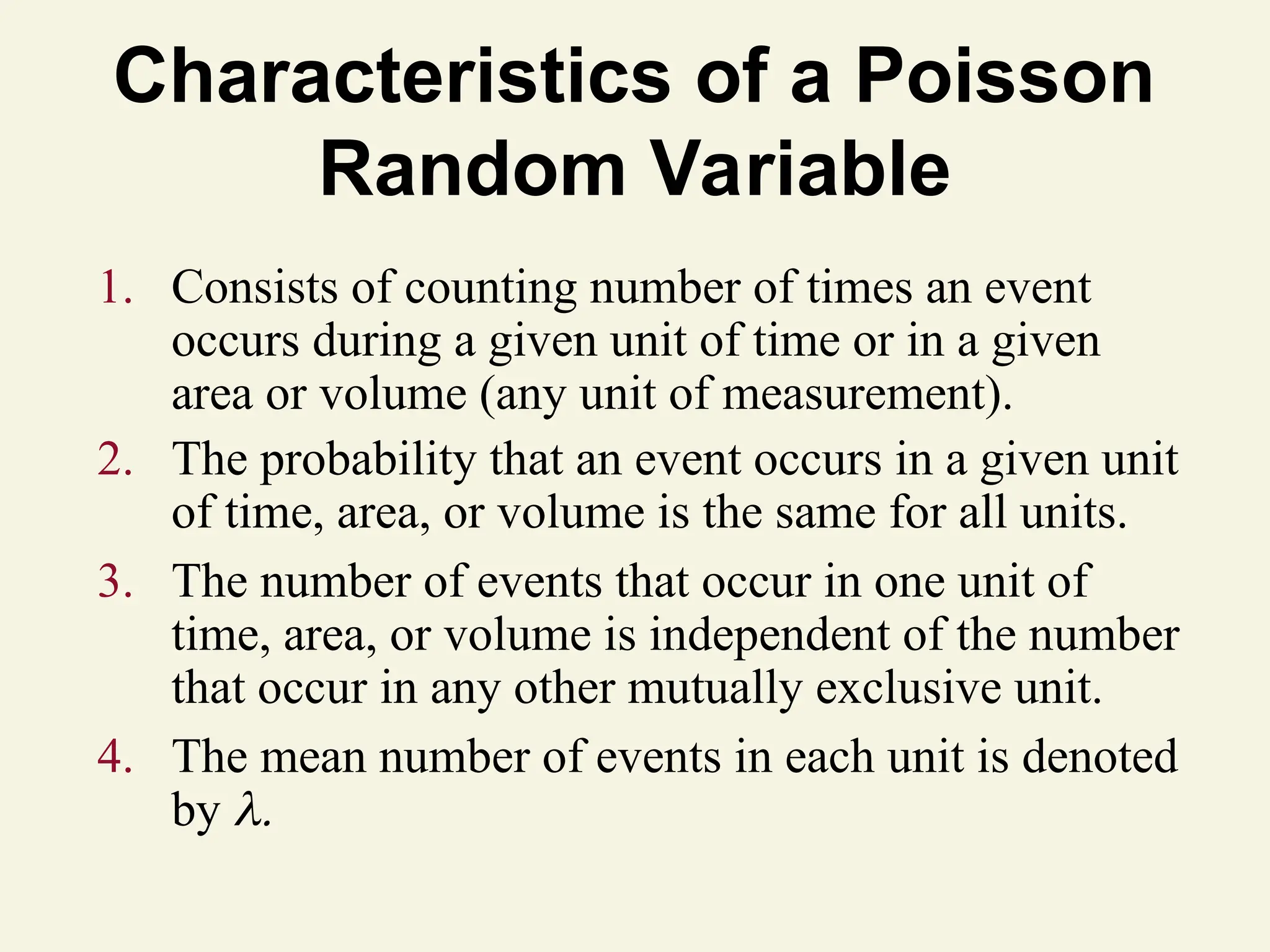
Characteristics of aPoisson
Random Variable
1. Consists of counting number of times an event
occurs during a given unit of time or in a given
area or volume (any unit of measurement).
2. The probability that an event occurs in a given unit
of time, area, or volume is the same for all units.
3. The number of events that occur in one unit of
time, area, or volume is independent of the number
that occur in any other mutually exclusive unit.
4. The mean number of events in each unit is denoted
by
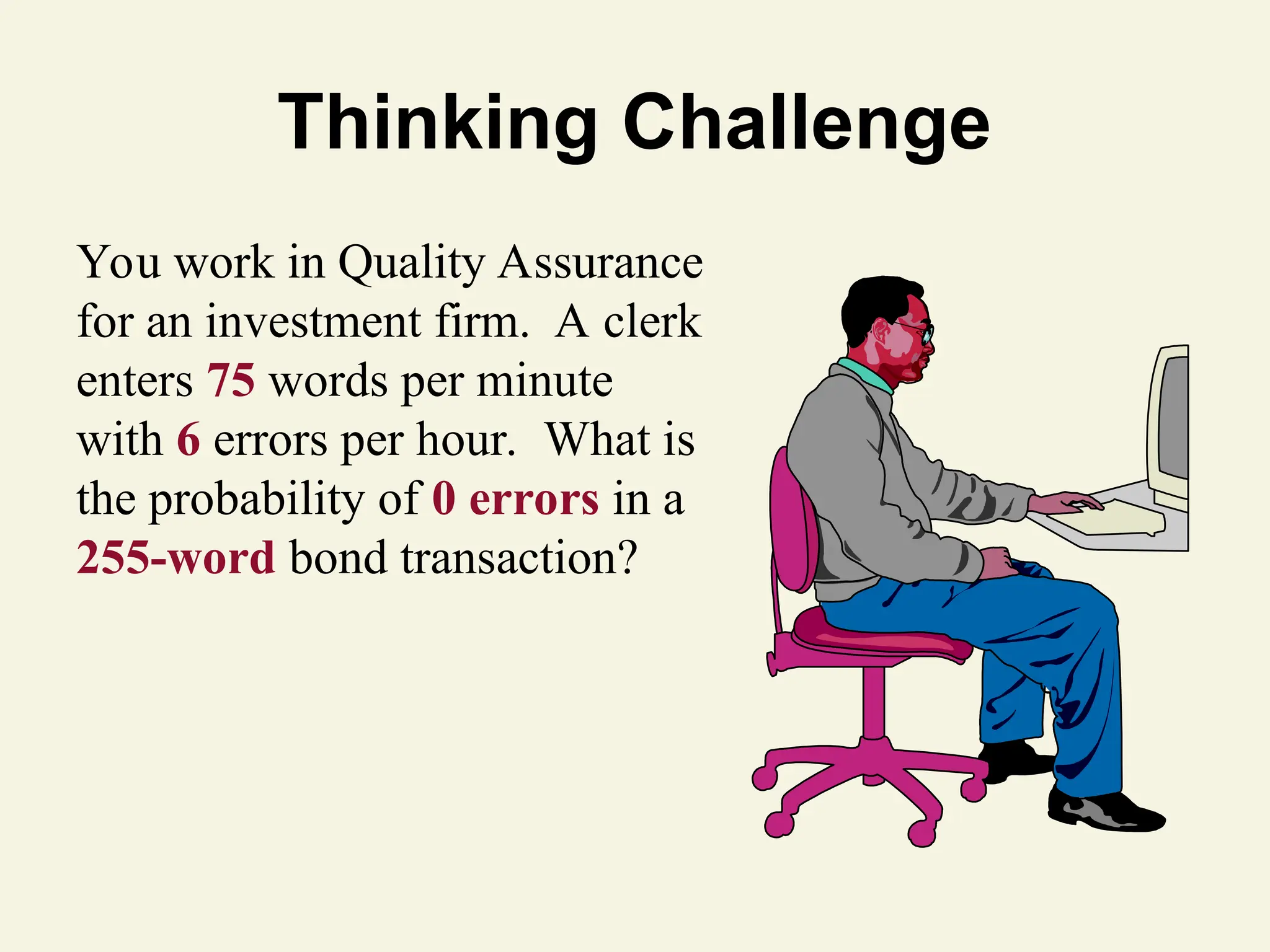
Thinking Challenge
You workin Quality Assurance
for an investment firm. A clerk
enters 75 words per minute
with 6 errors per hour. What is
the probability of 0 errors in a
255-word bond transaction?
46.
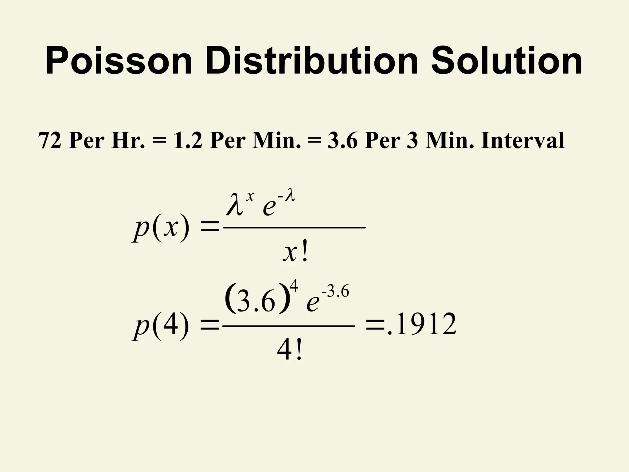
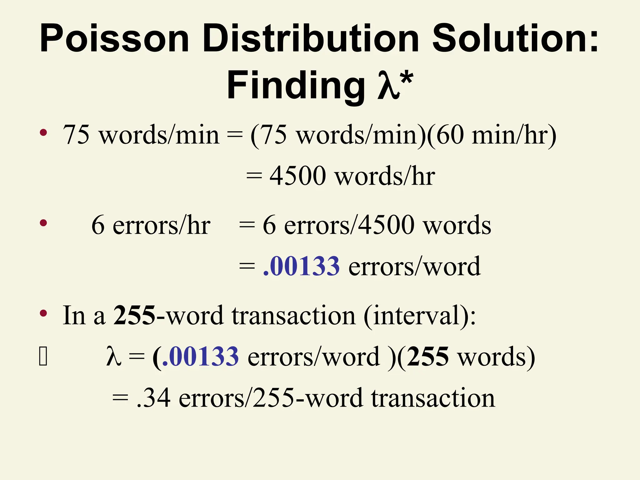
Poisson Distribution Solution:
Finding*
• 75 words/min = (75 words/min)(60 min/hr)
= 4500 words/hr
• 6 errors/hr = 6 errors/4500 words
= .00133 errors/word
• In a 255-word transaction (interval):
= (.00133 errors/word )(255 words)
= .34 errors/255-word transaction
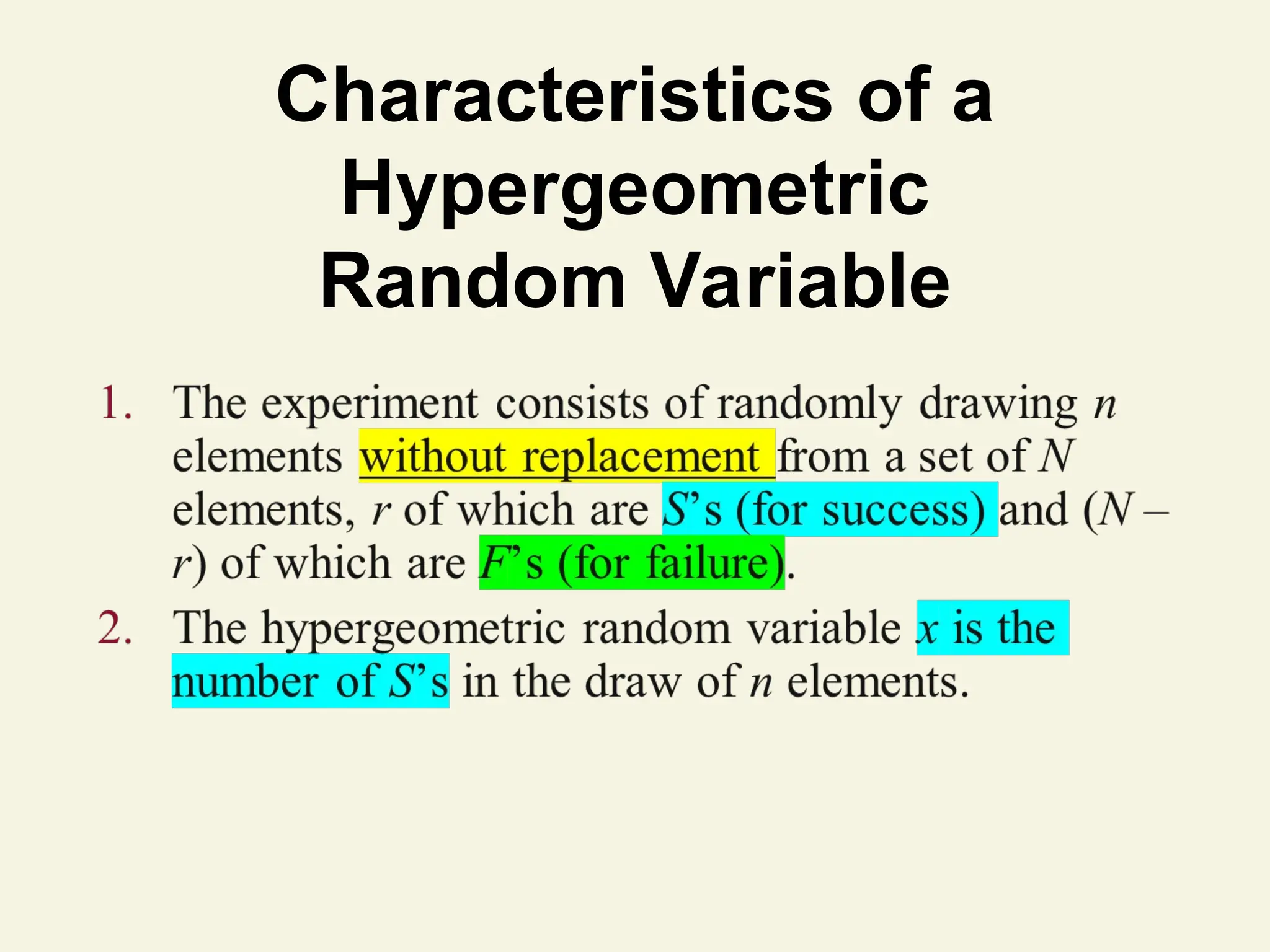
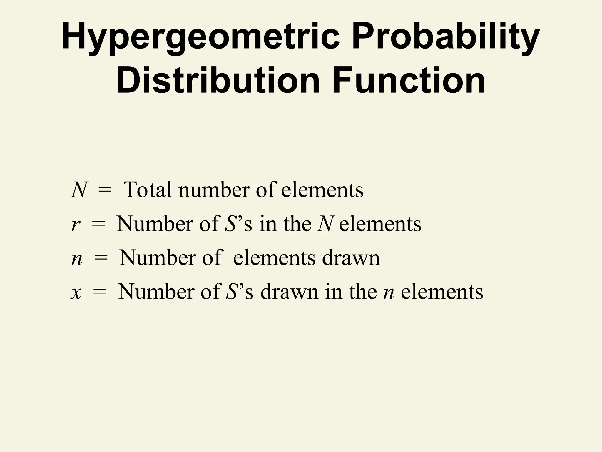
Hypergeometric Probability
Distribution Function
where. . .
[x = Maximum [0, n – (N – r), …,
Minimum (r, n)]
p x
r
x
N r
n x
N
n
µ
nr
N
2
r N r
n N n
N2
N 1
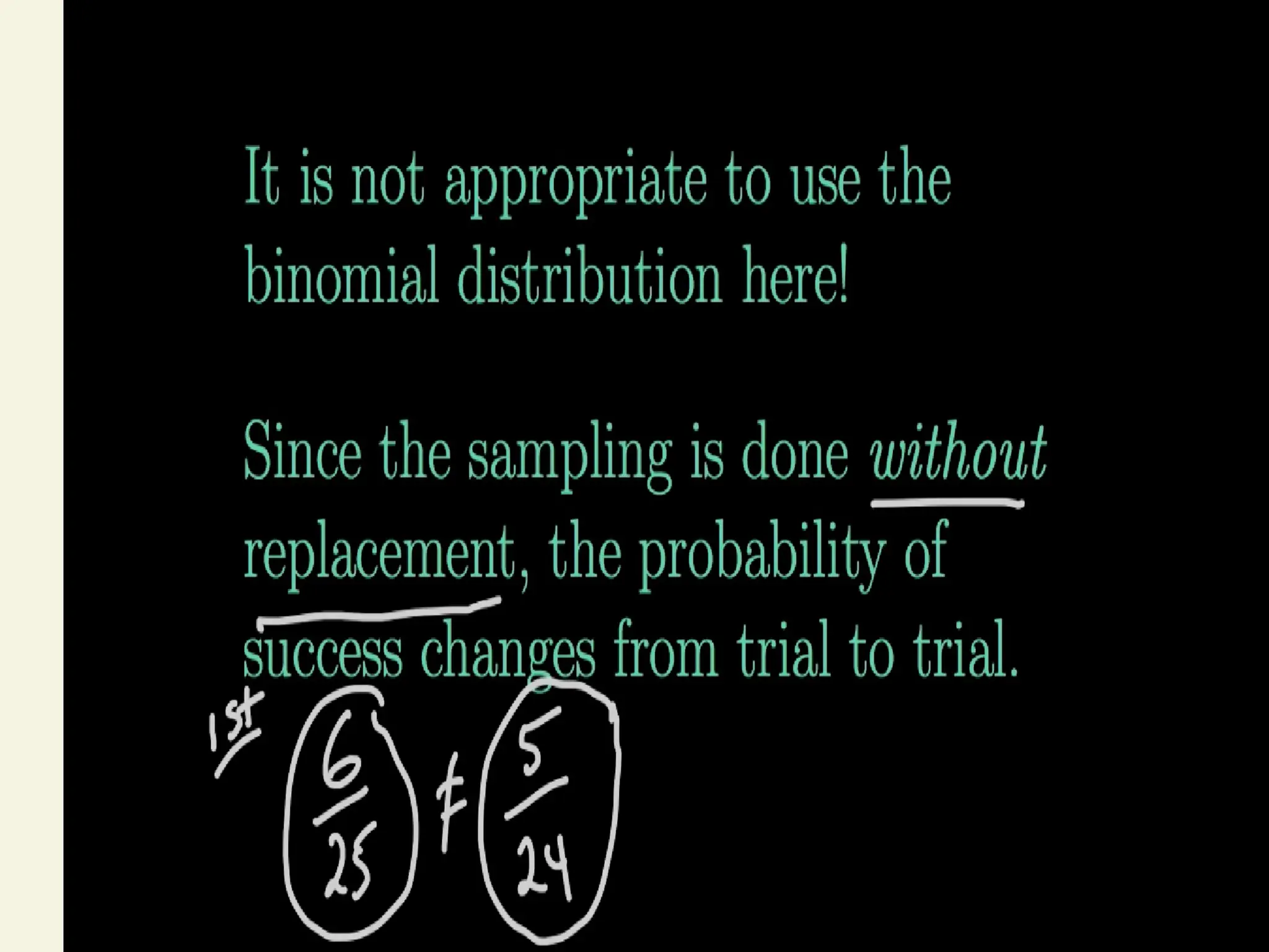
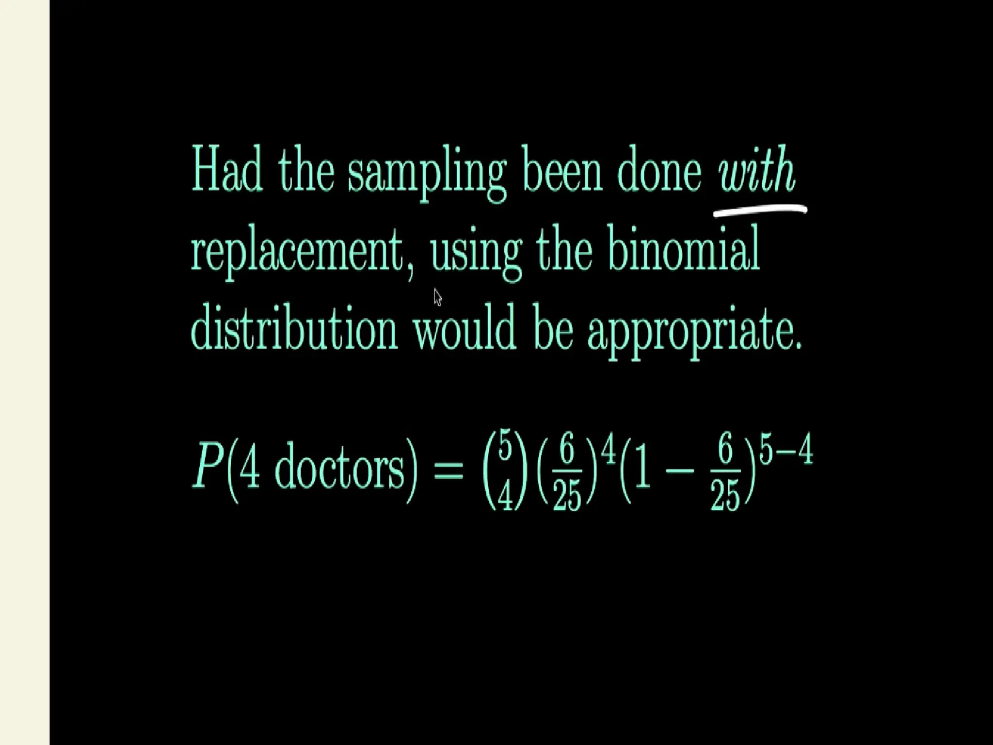
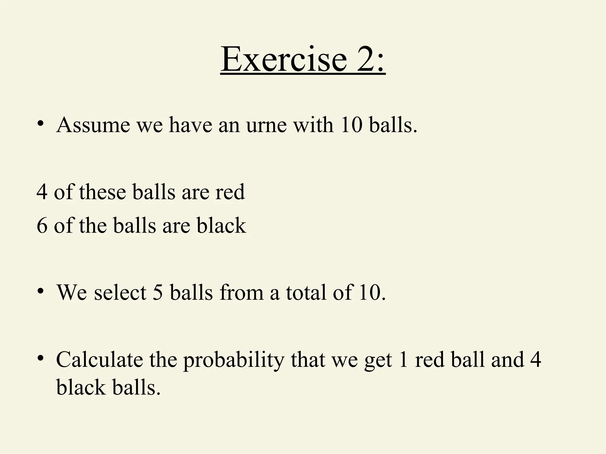
Exercise 2:
• Assumewe have an urne with 10 balls.
4 of these balls are red
6 of the balls are black
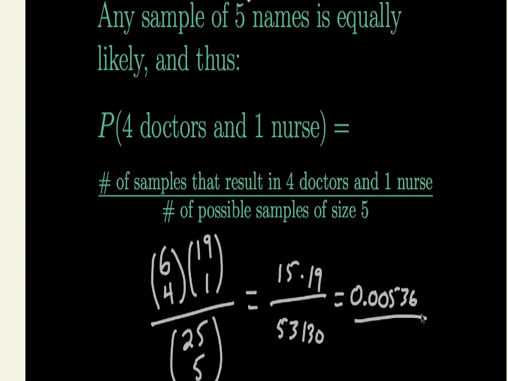
• We select 5 balls from a total of 10.
• Calculate the probability that we get 1 red ball and 4
black balls.
57.
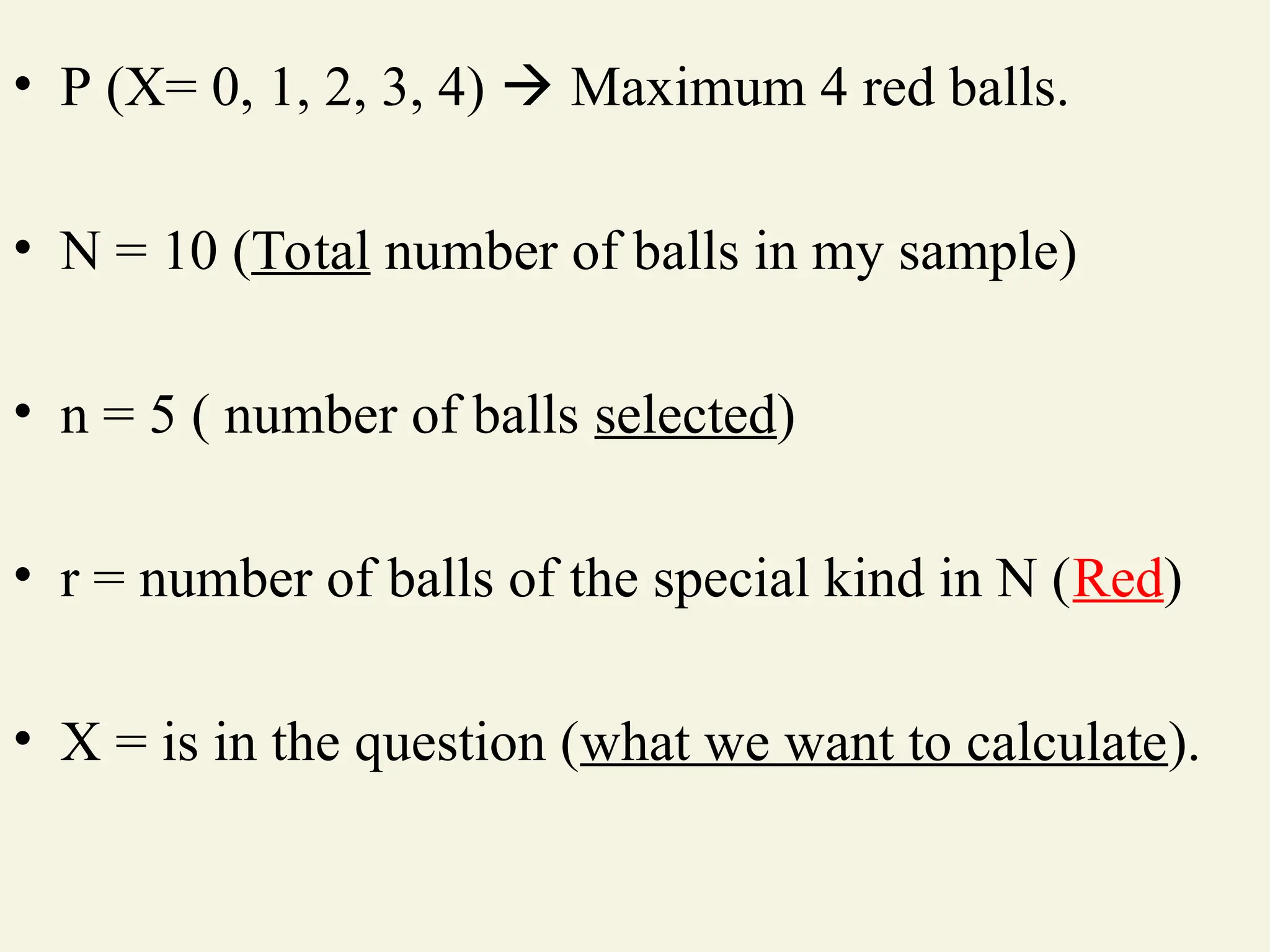
• P (X=0, 1, 2, 3, 4) Maximum 4 red balls.
• N = 10 (Total number of balls in my sample)
• n = 5 ( number of balls selected)
• r = number of balls of the special kind in N (Red)
• X = is in the question (what we want to calculate).
58.
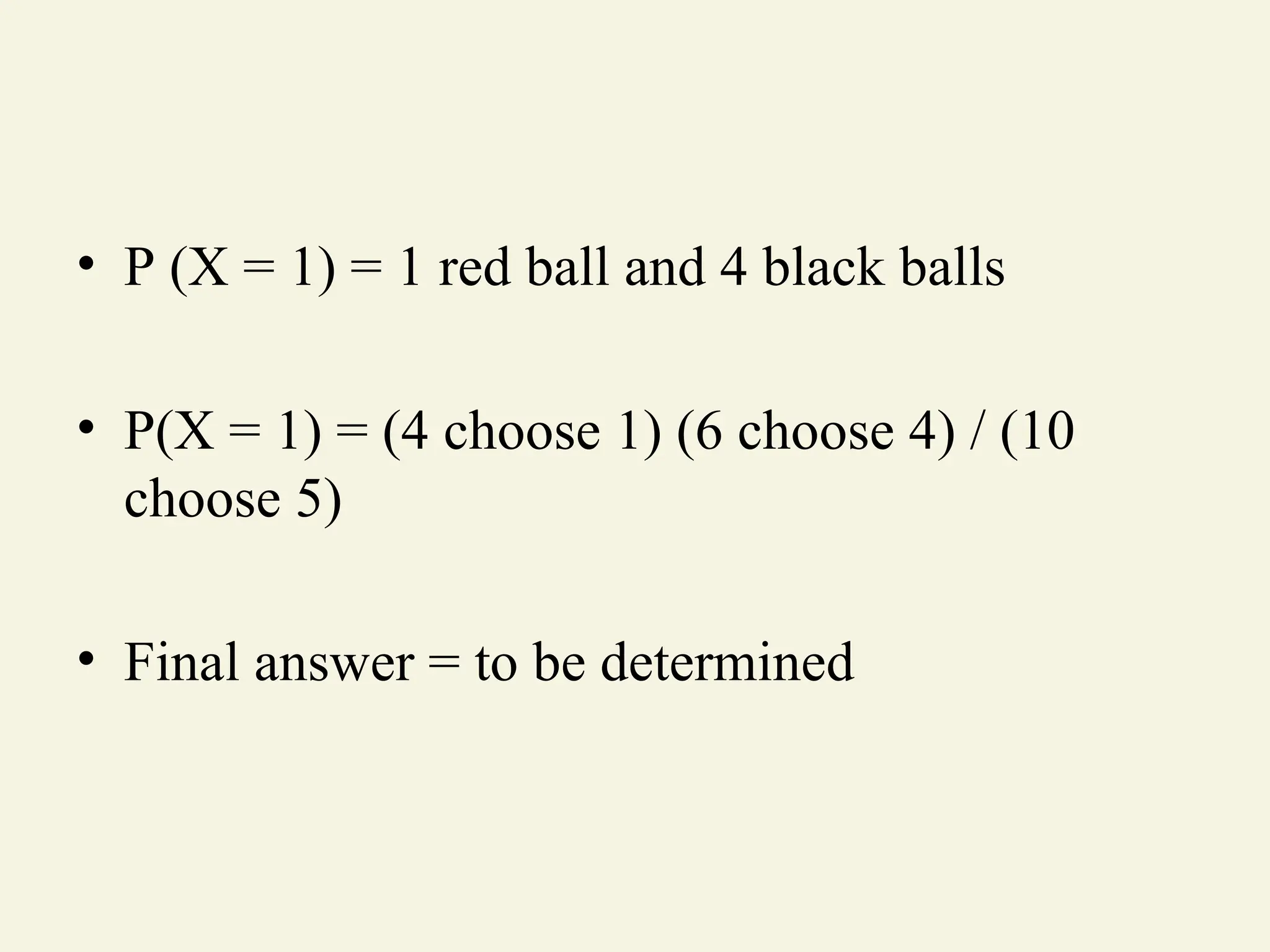
• P (X= 1) = 1 red ball and 4 black balls
• P(X = 1) = (4 choose 1) (6 choose 4) / (10
choose 5)
• Final answer = to be determined
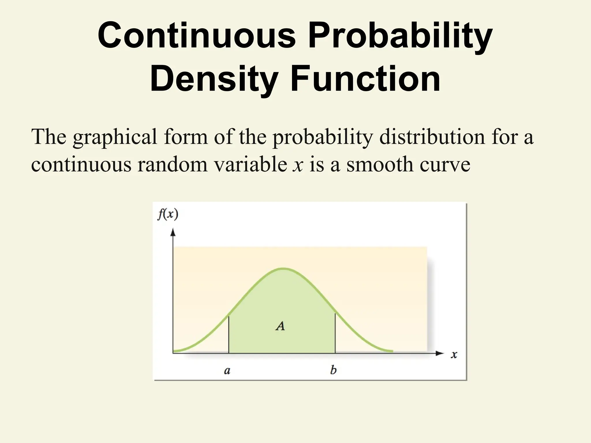
Continuous Probability
Density Function
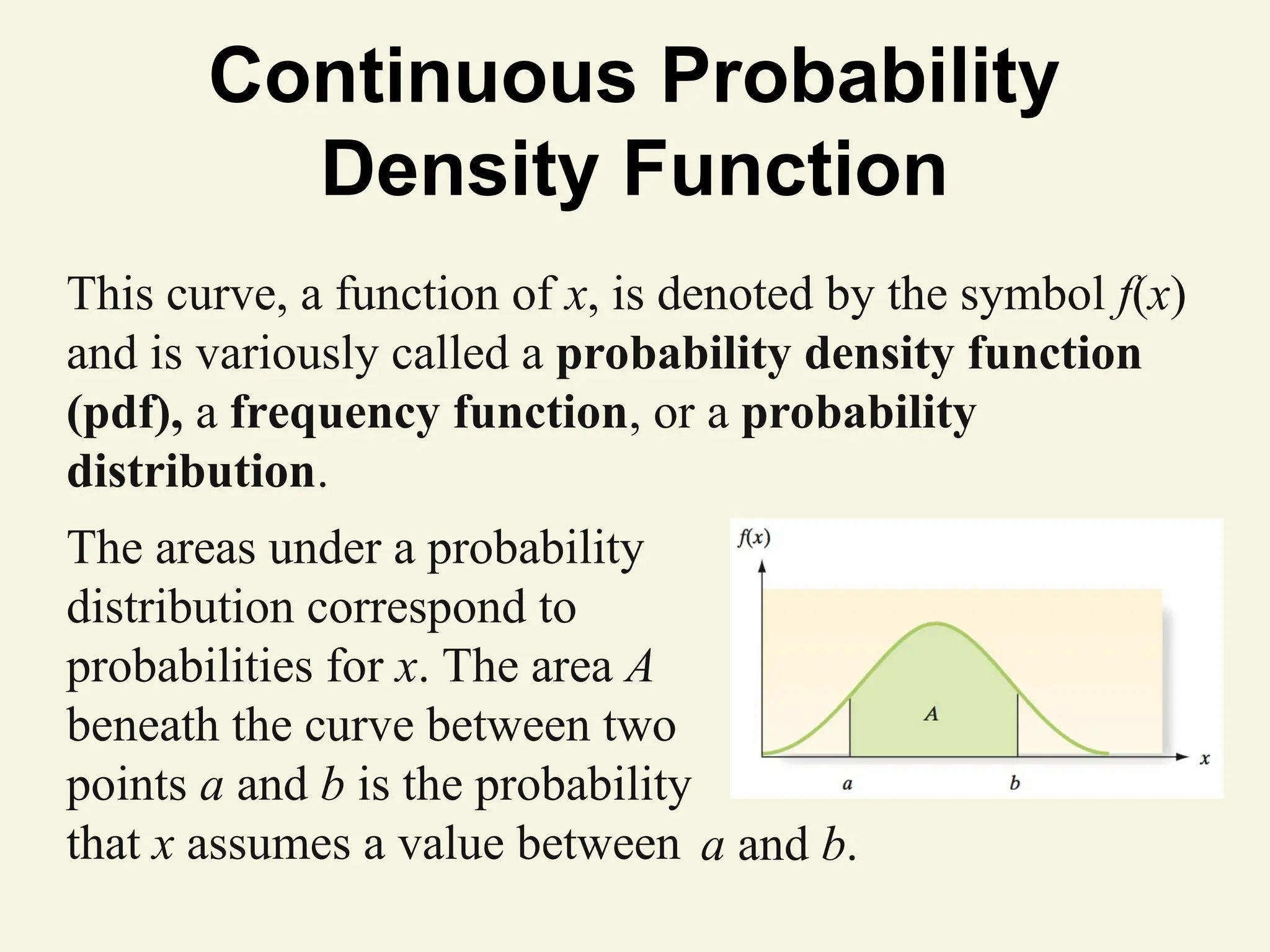
Thiscurve, a function of x, is denoted by the symbol f(x)
and is variously called a probability density function
(pdf), a frequency function, or a probability
distribution.
The areas under a probability
distribution correspond to
probabilities for x. The area A
beneath the curve between two
points a and b is the probability
that x assumes a value between a and b.
Editor's Notes
#2 As a result of this class, you will be able to...
#3 As a result of this class, you will be able to...
#4 As a result of this class, you will be able to...
#5 The ‘pass’ question is meant to be a ‘teaser’ and not answered.
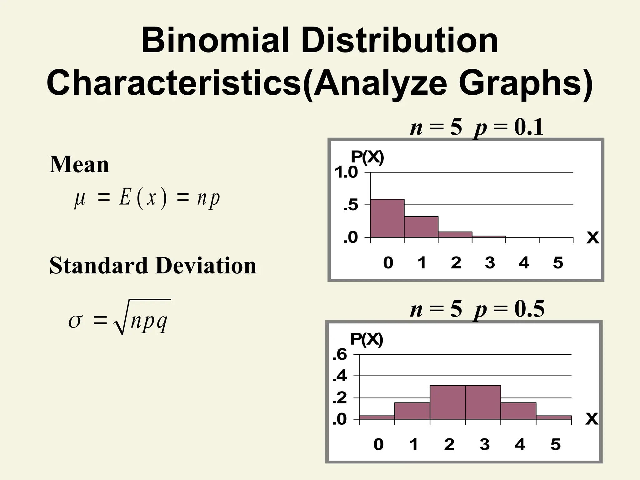
#31 Distribution has different shapes.
1st Graph:
If inspecting 5 items & the Probability of a defect is 0.1 (10%), the Probability of finding 0 defective item is about 0.6 (60%).
If inspecting 5 items & the Probability of a defect is 0.1 (10%), the Probability of finding 1 defective items is about .35 (35%).
2nd Graph:
If inspecting 5 items & the Probability of a defect is 0.5 (50%), the Probability of finding 1 defective items is about .18 (18%).
Note:
Could use formula or tables at end of text to get Probabilities.
#32 Let’s conclude this section on the binomial with the following Thinking Challenge.
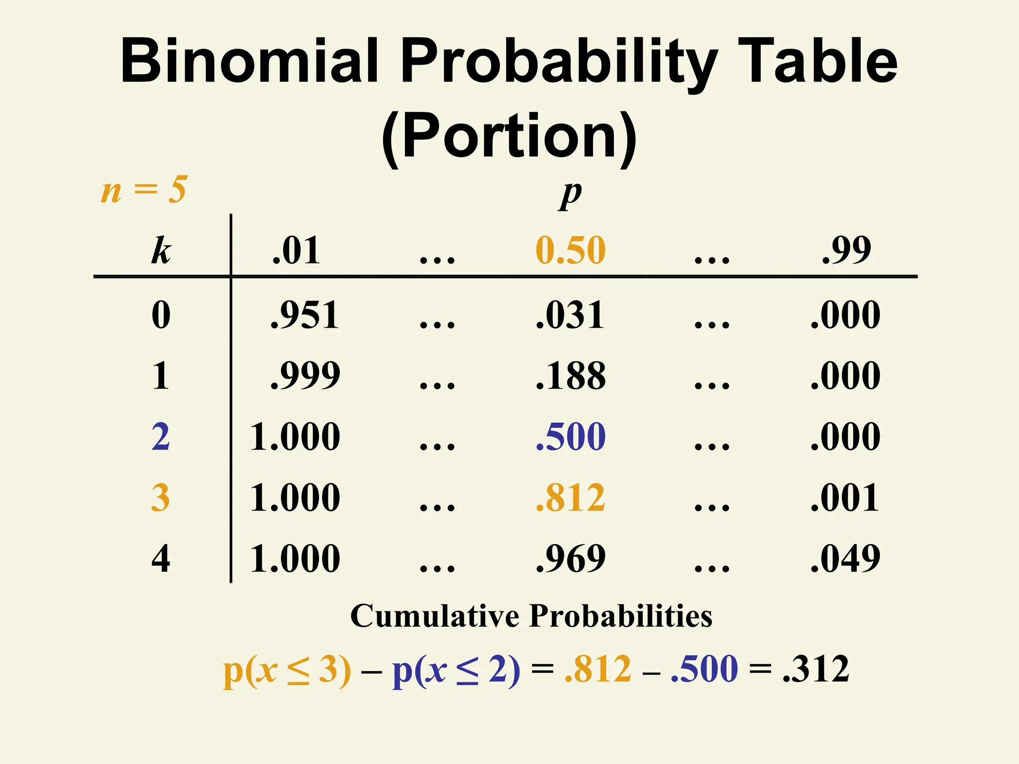
#33 From the Binomial Tables:
A. p(0) = .0687
B. p(2) = .2835
C. p(at most 2) = p(0) + p(1) + p(2)
= .0687+ .2062 + .2835
= .5584
D. p(at least 2) = p(2) + p(3)...+ p(12)
= 1 - [p(0) + p(1)]
= 1 - .0687 - .2062
= .7251
#38 Other Examples:
Number of machines that break down in a day
Number of units sold in a week
Number of people arriving at a bank teller per hour
Number of telephone calls to customer support per hour
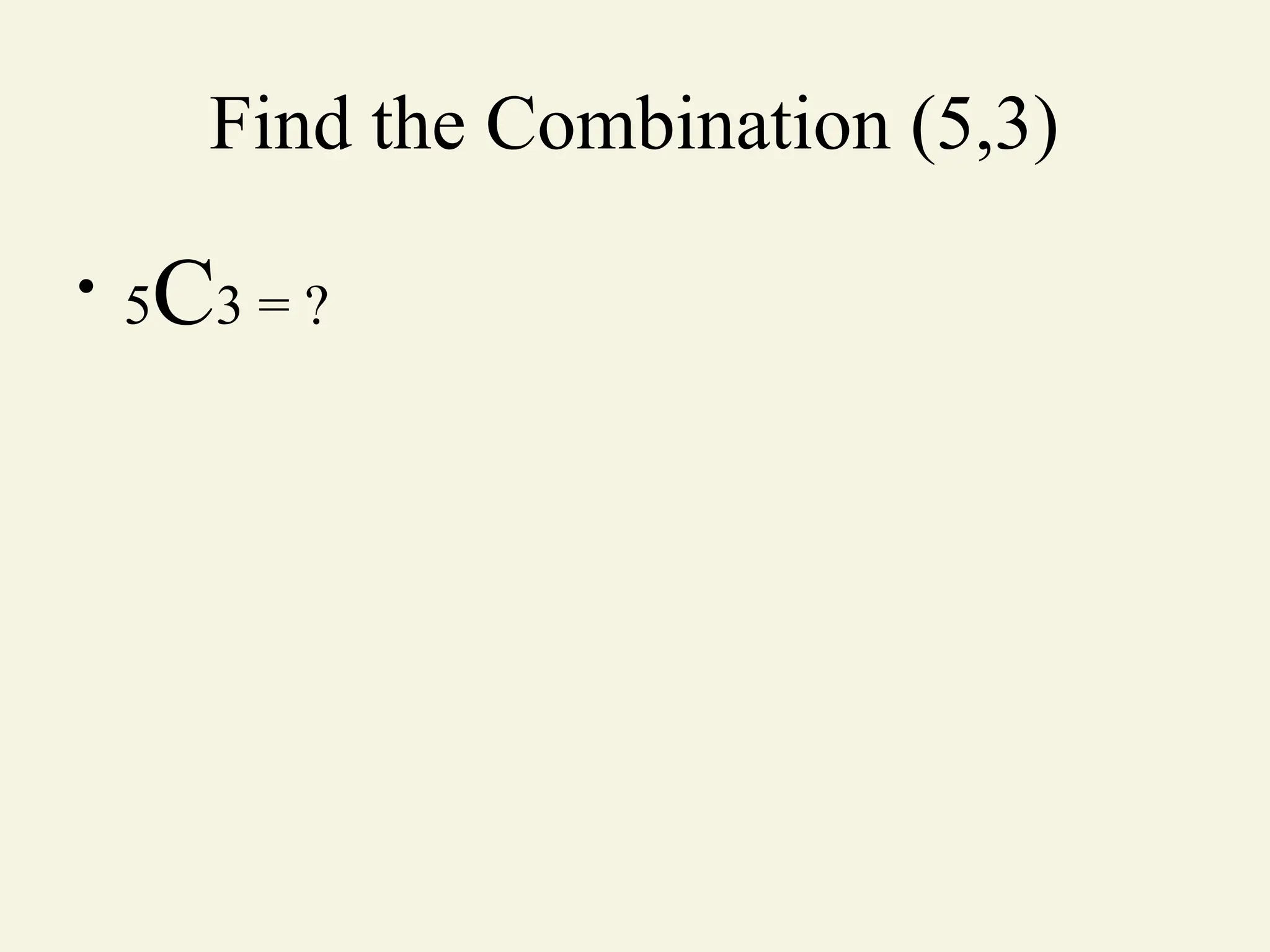
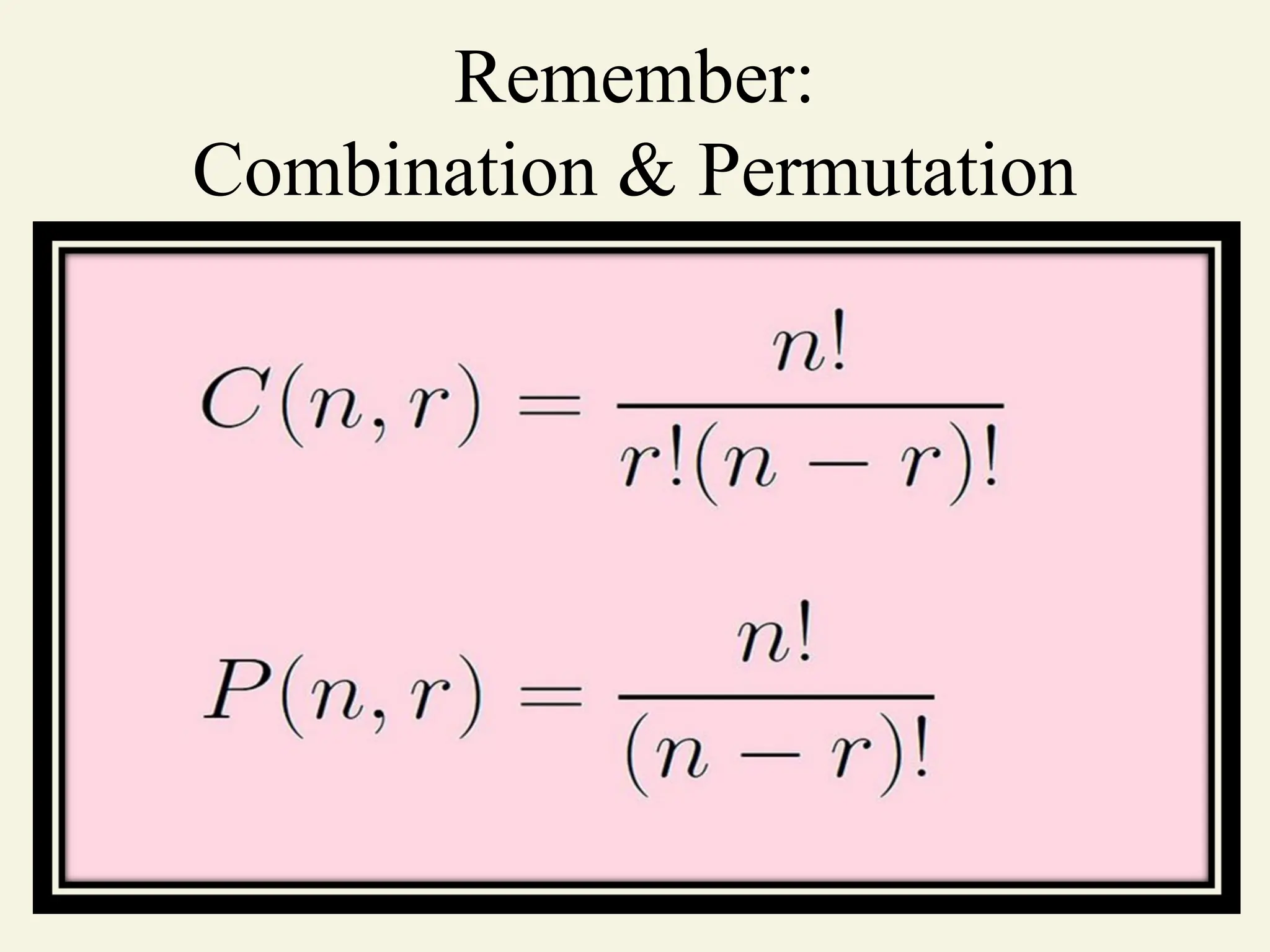
![nCx
• Combination 5C3 = 5!/[3!(5-3)!]=10](https://image.slidesharecdn.com/discreterandomvariablesprobdist4-251008070344-4a49ca9c/75/Discrete-Random-Variables-Prob-dist-4-0-pptx-28-2048.jpg)
![Binomial Distribution Solution*
n = 12, p = .20
A. p(0) = .0687
B. p(2) = .2835
C. p(at most 2) = p(0) + p(1) + p(2)
= .0687 + .2062 + .2835
= .5584
D. p(at least 2) = p(2) + p(3)...+ p(12)
= 1 – [p(0) + p(1)]
= 1 – .0687 – .2062
= .7251](https://image.slidesharecdn.com/discreterandomvariablesprobdist4-251008070344-4a49ca9c/75/Discrete-Random-Variables-Prob-dist-4-0-pptx-33-2048.jpg)

![Hypergeometric Probability
Distribution Function
where . . .
[x = Maximum [0, n – (N – r), …,
Minimum (r, n)]
p x
r
x
N r
n x
N
n
µ
nr
N
2
r N r
n N n
N2
N 1
](https://image.slidesharecdn.com/discreterandomvariablesprobdist4-251008070344-4a49ca9c/75/Discrete-Random-Variables-Prob-dist-4-0-pptx-49-2048.jpg)


![[DSC Europe 25] Vid Stimac - Policy Parsimony: Between Oversimplifying and Ov...](https://cdn.slidesharecdn.com/ss_thumbnails/eqlepagzqp2rhg3gbluh-dsc-stimac-251120-251205090438-059e7f54-thumbnail.jpg?width=640&height=640&fit=bounds)
![[DSC Europe 25] Max Talanov - Non digital NNs.pptx](https://cdn.slidesharecdn.com/ss_thumbnails/wif8tr3gtua74qvtopke-non-digital-nns-251205090438-26b0eea6-thumbnail.jpg?width=640&height=640&fit=bounds)
![[DSC Europe 25] Nikola Rajovic - Hardware Technologies Under the Hood: RISC-V...](https://cdn.slidesharecdn.com/ss_thumbnails/o2gptrmtoyqndgoshwgq-dsc2025-tenstorrent-rajovic-251205090438-814685f5-thumbnail.jpg?width=640&height=640&fit=bounds)


![[DSC Europe 25] Boris Perkovic - Lost in performance.pptx](https://cdn.slidesharecdn.com/ss_thumbnails/uq5hrp7vsuahqkxzifux-1-251204082258-fd2ee09d-thumbnail.jpg?width=640&height=640&fit=bounds)

![[DSC Europe 25] Marija Vlajkovic & Andrea Radonjanin - Integration of AI tool...](https://cdn.slidesharecdn.com/ss_thumbnails/qf1jrglttoc3bm8s3aop-final-integration-of-ai-tools-251208151905-394f3a6a-thumbnail.jpg?width=640&height=640&fit=bounds)


![[DSC Europe 25] Dragan Vucic - Building the Learning Organization - How AI Tr...](https://cdn.slidesharecdn.com/ss_thumbnails/8brigo2sbu6qur6gxrra-7-251205085715-6ae07d24-thumbnail.jpg?width=640&height=640&fit=bounds)


