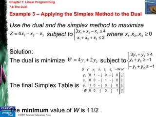
This chapter discusses linear programming problems and methods for solving them. It introduces linear inequalities in two variables and how to represent the feasible region geometrically. The chapter describes how to formulate a linear programming problem by defining the objective function and constraints. Solution methods covered include graphical representation, the simplex method, and its extensions like dealing with degeneracy, unbounded solutions, and minimization problems. The chapter also defines the dual of a linear programming problem and how to apply the simplex method to the dual problem.

1. INTRODUCTORY MATHEMATICALINTRODUCTORY MATHEMATICAL
ANALYSISANALYSISFor Business, Economics, and the Life and Social Sciences
©2007 Pearson Education Asia
Chapter 7Chapter 7
Linear ProgrammingLinear Programming

2. ©2007 Pearson Education Asia
INTRODUCTORY MATHEMATICAL
ANALYSIS
0. Review of Algebra
1. Applications and More Algebra
2. Functions and Graphs
3. Lines, Parabolas, and Systems
4. Exponential and Logarithmic Functions
5. Mathematics of Finance
6. Matrix Algebra
7. Linear Programming
8. Introduction to Probability and Statistics

3. ©2007 Pearson Education Asia
9. Additional Topics in Probability
10. Limits and Continuity
11. Differentiation
12. Additional Differentiation Topics
13. Curve Sketching
14. Integration
15. Methods and Applications of Integration
16. Continuous Random Variables
17. Multivariable Calculus
INTRODUCTORY MATHEMATICAL
ANALYSIS

4. ©2007 Pearson Education Asia
• To represent geometrically a linear inequality in two
variables.
• To state a linear programming problem and solve it
geometrically.
• To consider situations in which a linear programming
problem exists.
• To introduce the simplex method.
• To solve problems using the simplex method.
• To introduce use of artificial variables.
• To learn alteration of objective function.
• To define the dual of a linear programming problem.
Chapter 7: Linear Programming
Chapter ObjectivesChapter Objectives

5. ©2007 Pearson Education Asia
Linear Inequalities in Two Variables
Linear Programming
Multiple Optimum Solutions
The Simplex Method
Degeneracy, Unbounded Solutions, and Multiple Solutio
Artificial Variables
Minimization
The Dual
7.1)
7.2)
7.3)
7.4)
Chapter 7: Linear Programming
Chapter OutlineChapter Outline
7.5)
7.6)
7.7)
7.8)

6. ©2007 Pearson Education Asia
Chapter 7: Linear Programming
7.1 Linear Inequalities in 2 Variables7.1 Linear Inequalities in 2 Variables
• Linear inequality is written as
where a, b, c = constants and
not both a and b are zero.
0
or0
or0
or0
≥++
>++
≤++
<++
cbyax
cbyax
cbyax
cbyax

7. ©2007 Pearson Education Asia
Chapter 7: Linear Programming
7.1 Linear Inequalities in 2 Variables
• A solid line is included in the solution and a
dashed line is not.

8. ©2007 Pearson Education Asia
Chapter 7: Linear Programming
7.1 Linear Inequalities in 2 Variables
Example 1 – Solving a Linear Inequality
Example 3 – Solving a System of Linear Inequalities
Find the region defined by the inequality y ≤ 5.
Solution:
The region consists of the line y = 5
and with the half-plane below it.
Solve the system
Solution:
The solution is the unshaded region.



−≥
+−≥
2
102
xy
xy

9. ©2007 Pearson Education Asia
Chapter 7: Linear Programming
7.2 Linear Programming7.2 Linear Programming
Example 1 – Solving a Linear Programming Problem
• A linear function in x and y has the form
• The function to be maximized or minimized is
called the objective function.
byaxZ +=
Maximize the objective function Z = 3x + y subject
to the constraints
0
0
1232
82
≥
≥
≤+
≤+
y
x
yx
yx

10. ©2007 Pearson Education Asia
Chapter 7: Linear Programming
7.2 Linear Programming
Example 1 – Solving a Linear Programming Problem
Solution:
The feasible region is nonempty and bounded.
Evaluating Z at these points, we obtain
The maximum value of Z occurs when x = 4
and y = 0.
( ) ( )
( ) ( )
( ) ( )
( ) ( ) 4403
11233
12043
0003
=+=
=+=
=+=
=+=
DZ
CZ
BZ
AZ

11. ©2007 Pearson Education Asia
Chapter 7: Linear Programming
7.2 Linear Programming
Example 3 – Unbounded Feasible Region
The information for a produce is summarized as
follows:
If the grower wishes to minimize cost while still
maintaining the nutrients required, how many bags of
each brand should be bought?

12. ©2007 Pearson Education Asia
Chapter 7: Linear Programming
7.2 Linear Programming
Example 3 – Unbounded Feasible Region
Solution:
Let x = number of bags of Fast Grow bought
y = number of bags of Easy Grow bought
To minimize the cost function
Subject to the constraints
There is no maximum value
since the feasible region is unbounded .
yxC 68 +=
0
0
802
20025
16023
≥
≥
≥+
≥+
≥+
y
x
yx
yx
yx

13. ©2007 Pearson Education Asia
Chapter 7: Linear Programming
7.3 Multiple Optimum Solutions7.3 Multiple Optimum Solutions
Example 1 – Multiple Optimum Solutions
• There may be multiple optimum solutions for an
objective function.
Maximize Z = 2x + 4y subject
to the constraints
Solution:
The region is nonempty and bounded.
0,
162
84
≥
≤+
−≤−
yx
yx
yx
( ) ( ) ( )
( ) ( ) ( )
( ) ( ) ( ) (max)328402
(max)324482
82402
=+=
=+=
=+=
CZ
BZ
AZ

14. ©2007 Pearson Education Asia
Chapter 7: Linear Programming
7.4 The Simplex Method7.4 The Simplex Method
Standard Linear Programming Problem
• Maximize the linear function
subject to the constraints
where x and b are non-negative.
nn xcxcxcZ +++= 2211










≤+++
≤+++
≤+++
≤+++
mnmnmm
nn
nn
nn
bxaxaxa
bxaxaxa
bxaxaxa
bxaxaxa




2211
11212111
11212111
11212111
.
.

15. ©2007 Pearson Education Asia
Chapter 7: Linear Programming
7.4 The Simplex Method
Example 1 – The Simplex Method
Maximize subject to and
x1, x2 ≥ 0.
Solution:
The maximum value of Z is 95.





≤+−
≤+
≤+
123
352
20
21
21
21
xx
xx
xx
21 45 xxZ +=














−−
−
0
12
35
20
100045
000013
001012
000111
3
2
1
32121
Z
s
s
s
RZsssxxB














−
−
−
95
52
15
5
101300
014500
001101
001210
3
1
2
32121
Z
s
x
x
RZsssxxB

16. ©2007 Pearson Education Asia
Chapter 7: Linear Programming
7.5 Degeneracy, Unbounded and Multiple Solutions7.5 Degeneracy, Unbounded and Multiple Solutions
Degeneracy
• A basic feasible solution (BFS) is degenerate if one
of the basic variables is 0.
Unbounded Solutions
• An unbounded solution occurs when the objective
function has no maximum value.
Multiple Optimum Solutions
• Multiple (optimum) solutions occur when there are
different BFS.

17. ©2007 Pearson Education Asia
Chapter 7: Linear Programming
7.5 Degeneracy, Unbounded and Multiple Solutions
Example 1 – Unbounded Solution
Maximize subject to
Solution:
Since the 1st
two rows of the x1-column are negative,
no quotients exist.
Hence, it has an unbounded solution.
321 4 xxxZ −+=





≥
≤++−
≤−+−
0,,
1263
30265
321
321
321
xxx
xxx
xxx










0
12
30
1001-4-1-
010631-
0012-65-
Z
s
s
2
1
32121 RZsssxxB










16
4
6
1090-
0021-
02-114-03-
3
4
3
7
3
1
3
1
2
1
32121
Z
x
s
RZsssxxB

18. ©2007 Pearson Education Asia
Chapter 7: Linear Programming
7.6 Artificial Variables7.6 Artificial Variables
Example 1 – Artificial Variables
• Use artificial variables to handle maximization
problems that are not of standard form.
Maximize subject to
Solution:
Add an artificial variable t,
Consider an artificial objective equation,
212 xxZ +=







≥
≥+−
≤+
≤+
0,
2
202
12
21
21
21
21
xx
xx
xx
xx
2
202
12
321
221
121
=+−+−
=++
=++
tsxx
sxx
sxx
02 21 =++−− WMtxx

19. ©2007 Pearson Education Asia
Construct a Simplex Table,
All indicators are nonnegative.
The maximum value of Z is 17.












−−−+−
−−
MMMMW
t
s
s
RWtsssxxB
2100012
20110011
200001021
120000111
2
1
3212`












−
−
171000
70010
10100
50001
2
1
2
3
2
1
2
1
2
1
2
3
2
1
2
1
2
1
3212`
W
t
s
s
RZsssxxB
Chapter 7: Linear Programming
7.6 Artificial Variables
Example 1 – Artificial Variables

20. ©2007 Pearson Education Asia
Use the simplex method to maximize
subject to
Solution:
Construct a Simplex Table,
The feasible region is empty, hence, no solution
exists.










−++−
−−−
MMMMW
s
t
RWtssxxB
1101021
1001011
1011102
2
1
12121










−−−+−
−−
MMMMW
s
t
RWtssxxB
210012
1001011
2010111
2
1
12121
Chapter 7: Linear Programming
7.6 Artificial Variables
Example 3 – An Empty Feasible Region
2132 xxZ =





≥
≤+
≥+−
0,
1
2
21
21
21
xx
xx
xx

21. ©2007 Pearson Education Asia
Chapter 7: Linear Programming
7.7 Minimization7.7 Minimization
Example 1 – Minimization
• To minimize a function is to maximize the negative
of the function.
Minimize subject to
Solution:
Construct a Simplex Table,
The minimum value of Z is −(−4) = 4.
21 2xxZ +=





≥
≥+−
≥+−
0,
2
12
21
21
21
xx
xx
xx










−−+
−
−−
MMMMMW
t
t
RWttssxxB
31002231
20101011
10010112
2
1
212121










−+−
−−−
−−
4122003
10111101
20101011
2
1
212121
MMW
t
t
RWttssxxB

22. ©2007 Pearson Education Asia
Chapter 7: Linear Programming
7.8 The Dual7.8 The Dual
Example 1 – Finding the Dual of a Maximization Problem
Find the dual of the following:
Maximize subject to
where
Solution:
The dual is minimize subject to
where
321 243 xxxZ ++=



≤++
≤+
1022
102
321
21
xxx
xx
21 1010 yyW +=





−≥−
≥+−
≥−
34
1
23
21
21
21
xx
xx
xx
0,, 321 ≥xxx
0, 21 ≥yy

23. ©2007 Pearson Education Asia
Chapter 7: Linear Programming
7.8 The Dual
Example 3 – Applying the Simplex Method to the Dual
Use the dual and the simplex method to maximize
subject to where
Solution:
The dual is minimize subject to
The final Simplex Table is
The minimum value of W is 11/2 .
21 24 yyW +=
0,, 321 ≥xxx3214 xxxZ −−=



≤++
≤−+
2
43
321
321
xxx
xxx




−≥+−
−≥+
≥+
1
1
43
21
21
21
yy
yy
yy












−
−−
−−
−
−
2
11
2
1
2
3
4
5
4
1
4
1
2
5
2
1
2
1
4
1
4
3
4
1
1
2
2
32121
1000
0001
0100
0010
W
y
s
y
RWsssyyB