Basic Derivation

1. Derivatives And It’s Simple Applications

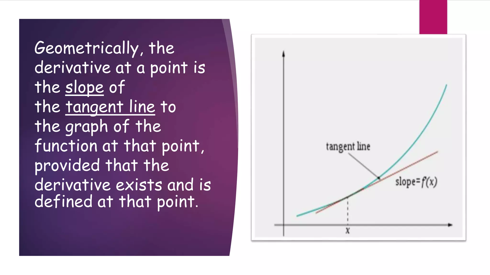
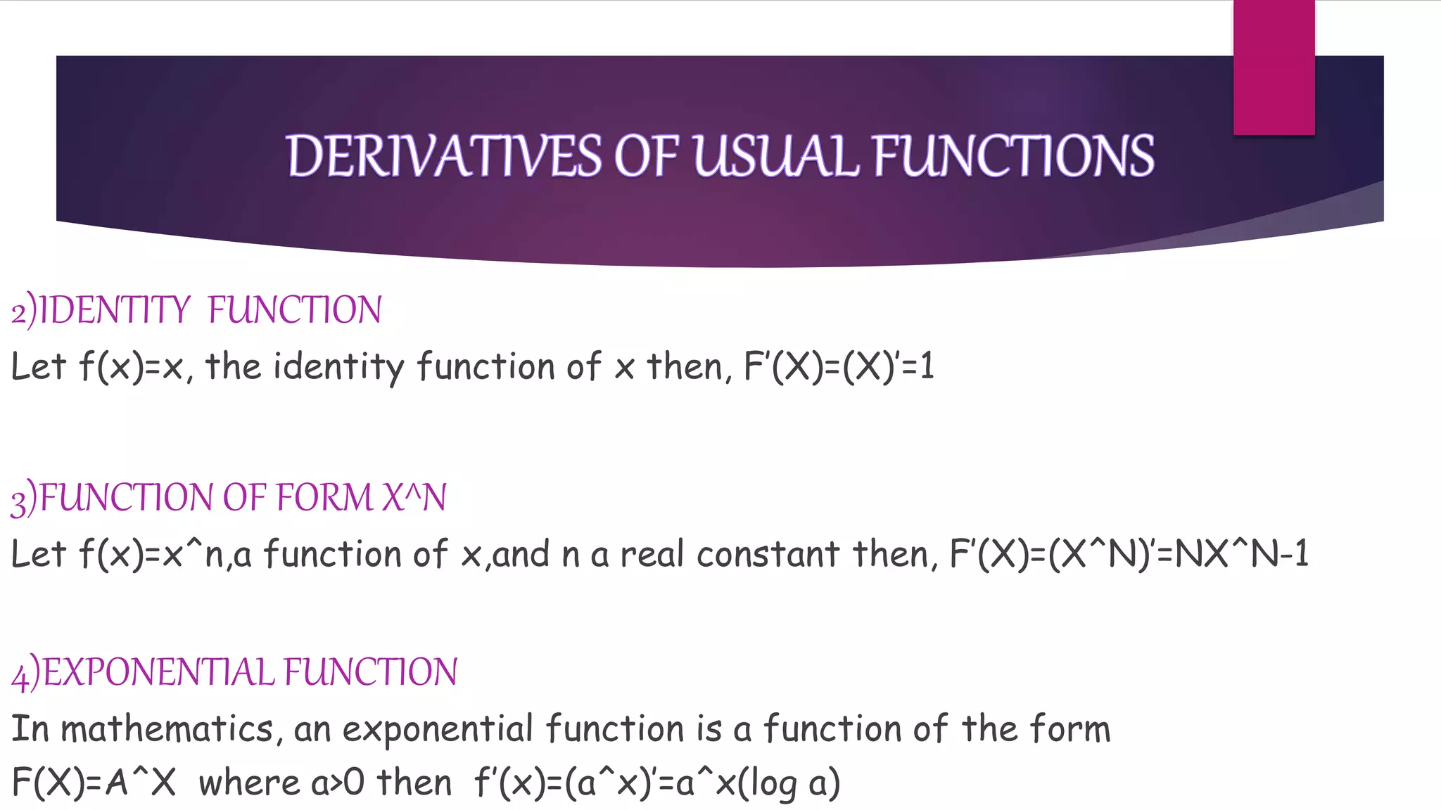
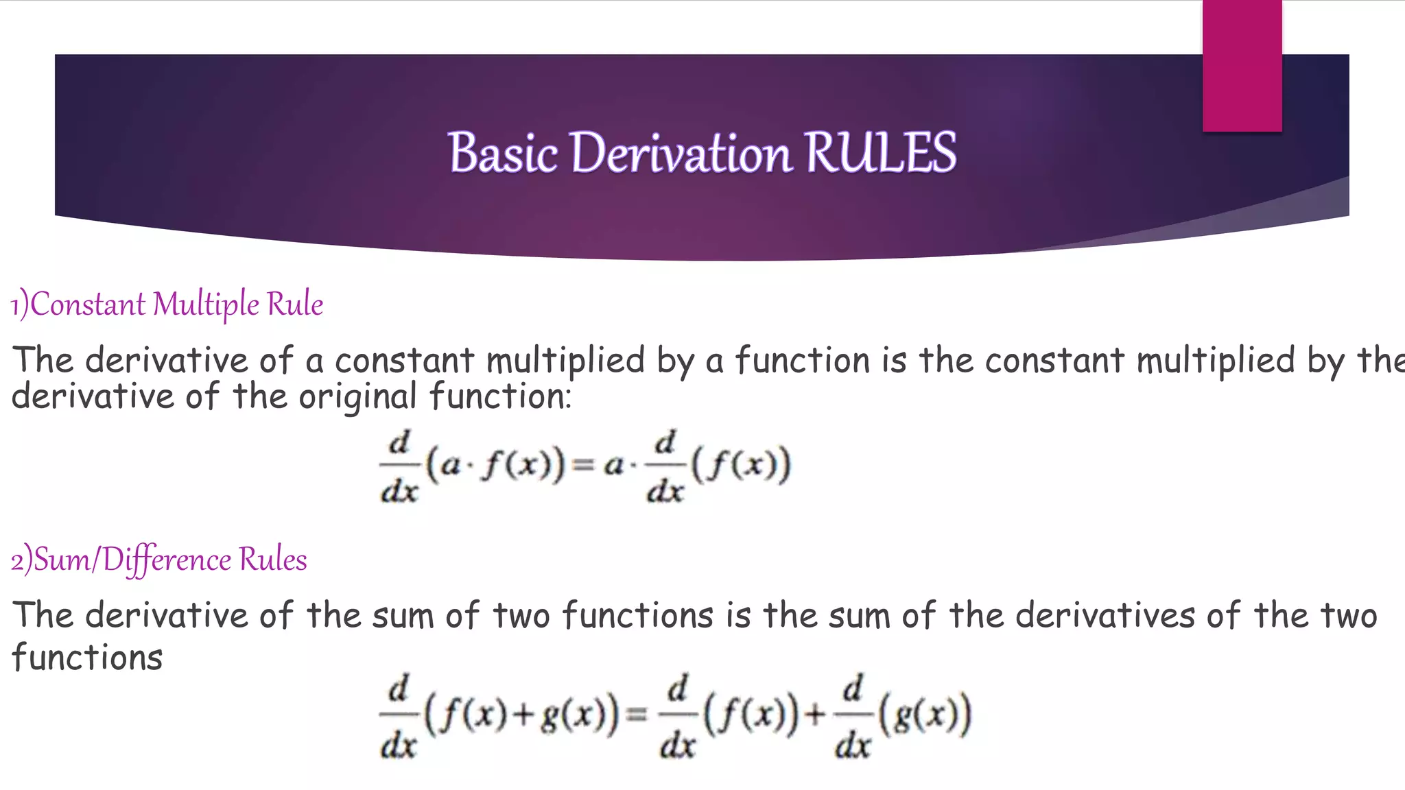
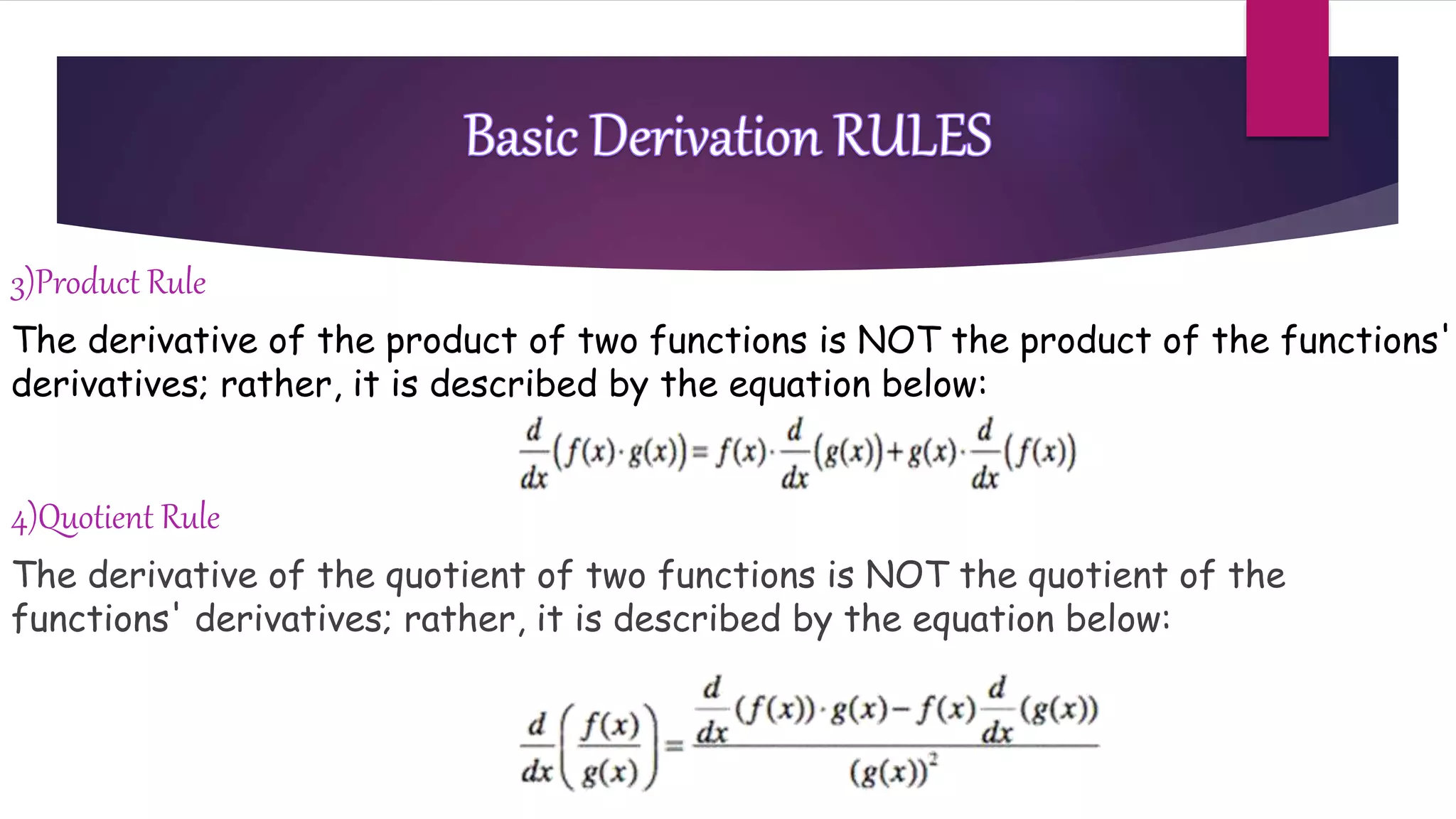
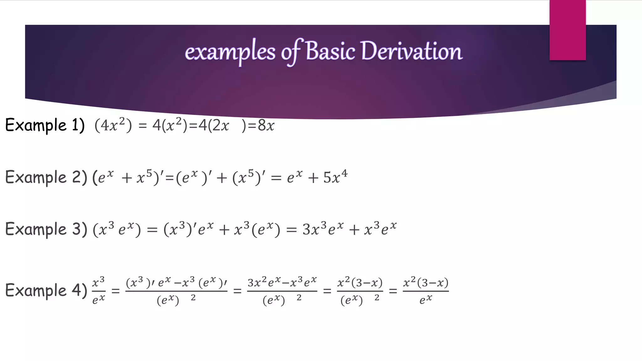
4. Introduction to derivative
 In mathematics, differential calculus is a subfield of calculus concerned with the study
of the rates at which quantities change.
 The primary objects of study in differential calculus are the derivative of a function,
related notions such as the differential, and their applications.
 The derivative of a function at a chosen input value describes the rate of change of the
function near that input value. The process of finding a derivative is
called differentiation

5. Geometrically, the
derivative at a point is
the slope of
the tangent line to
the graph of the
function at that point,
provided that the
derivative exists and is
defined at that point.

6. Derivative of usual function

7. 1) Differentiating Constant Functions
Remember that a constant function has the same value at every point. The graph of
such a function is a horizontal line:
Now at any point, the tangent line to the graph (remember this is the line which
best approximates the graph) is the same horizontal line. Since the derivative
measures the slope of the tangent line and a horizontal line has slope zero, we
expect the following:
Derivative of a constant :

8. 2)IDENTITY FUNCTION
Let f(x)=x, the identity function of x then, F’(X)=(X)’=1
3)FUNCTION OF FORM X^N
Let f(x)=x^n,a function of x,and n a real constant then, F’(X)=(X^N)’=NX^N-1
4)EXPONENTIAL FUNCTION
In mathematics, an exponential function is a function of the form
F(X)=A^X where a>0 then f’(x)=(a^x)’=a^x(log a)

9. Basic derivation rules

10. 1)Constant Multiple Rule
The derivative of a constant multiplied by a function is the constant multiplied by the
derivative of the original function:
2)Sum/Difference Rules
The derivative of the sum of two functions is the sum of the derivatives of the two
functions

11. 3)Product Rule
The derivative of the product of two functions is NOT the product of the functions'
derivatives; rather, it is described by the equation below:
4)Quotient Rule
The derivative of the quotient of two functions is NOT the quotient of the
functions' derivatives; rather, it is described by the equation below:

12. Let us see some examples to understand how Basic
rules of derivatives are applied

13. Example 1) 4𝑥2 = 4(𝑥2)=4(2𝑥 )=8𝑥
Example 2) (𝑒 𝑥
+ 𝑥5
)′=(𝑒 𝑥
)′ + (𝑥5
)′ = 𝑒 𝑥
+ 5𝑥4
Example 3) (𝑥3 𝑒 𝑥) = 𝑥3 ′ 𝑒 𝑥 + 𝑥3(𝑒 𝑥) = 3𝑥3 𝑒 𝑥 + 𝑥3 𝑒 𝑥
Example 4)
𝑥3
𝑒 𝑥 =
(𝑥3 )′ 𝑒 𝑥 −𝑥3 (𝑒 𝑥 )′
(𝑒 𝑥) 2 =
3𝑥2 𝑒 𝑥−𝑥3 𝑒 𝑥
(𝑒 𝑥) 2 =
𝑥2 3−𝑥
(𝑒 𝑥) 2 =
𝑥2 3−𝑥
𝑒 𝑥

15. THE CHAIN RULE
The chain rule is a formula for computing the derivative of
the composition of two or more function.
That is, if f and g are functions, then the chain rule expresses the
derivative of their composition f o g
The function which maps x to f(g(x)) in terms of the derivatives
of f and g and the product of function as follows:
(f o g)’=(f’ o g).g’

16. A function inverse can be thought of as the reversal of whatever our function does
to its input. Composition of two inverse function results in identity function. Inverse
of inverse of a function is that function itself
where (f o f−1)(x) = (f−1o f)(x)
Steps to solve inverse function is summarized below.
•On both sides of the equation replace x with f−1 (x).
•Substitute f(f−1(x)) = x
•Solve f−1 (x) in terms of x.

17. Let us see some examples to understand How
composite function are applied

18. Example 1: Find the derivative of Sin 10x
Solution:
Let y = sin u and u = 10x
dy
dx
= cos u and
du
dx
= 10
Hence
dy
dx
=
dy
du
∗
du
dx
= cos u * 10 = 10 cos 10x

19. Example 2:The two functions f and g are defined on the set of real numbers such
that: f(x)= 𝑥2
+ 5 and g(x) = x√x. Find fog and gof and show that fog≠gof.
Solution :
(fog)(x) = f{g(x)} (fog)(x) = f(x√x) = √𝑥
2
+ 5 = x + 5
(gof)(x) = g(f(x) (gof)(x) = g(𝑥2+ 5) = x2 + 5
Therefore fog ≠ gof

21. In calculus, the second derivative, or the second order derivative, of a function f is
the derivative of the derivative of f.
Roughly speaking, the second derivative measures how the rate of change of a
quantity is itself changing
for example, the second derivative of the position of a vehicle with respect to time
is the instantaneous acceleration of the vehicle, or the rate at which the velocity of
the vehicle is changing with respect to time.
In Leibniz notation:
𝑎 =
𝑑𝑣
𝑑𝑡
=
𝑑 2∗𝑥
𝑑𝑡 2 where the last term is the second derivative expression.

22. Second derivative test
The relation between the second
derivative and the
Graph can be used to test whether a
stationary point for a
Function is a local maximum or a local
minimum.
Specifically
If f’’(x) <0 then f has a local
maximum at x.
If f’’(x)>0 then f has a local
minimum at x.
If f’’(x)=0 , the second derivative
test says nothing
about the point x , a possible
inflection point.

23. Second derivative test
The reason the second derivative produces these results can be seen by way of a
real-world analogy. Example,
Consider a vehicle that at first is moving forward at a great velocity, but with a
negative acceleration.
Clearly the position of the vehicle at the point where the velocity reaches zero will
be the maximum distance from the starting position – after this time, the velocity
will become negative and the vehicle will reverse.
The same is true for the minimum, with a vehicle that at first has a very negative
velocity but positive acceleration.

24. Let us see some examples to understand how
application of derivatives takes place

25. In physics
A particle is moving in such a way that its displacement ‘s’ at a time ‘t’ is
given by 𝒔 = 𝟐𝒕 𝟐 + 𝟓𝒕 + 𝟐𝟎, find the velocity and acceleration after 2 sec.
Solution :
𝑠 = 2𝑡2 + 5𝑡 + 20 Therefore velocity =
𝑑𝑠
𝑑𝑡
= 4𝑡 + 5
𝑑𝑠
𝑑𝑡
= 4(2) + 5 =13
Acceleration = a =
𝑑𝑣
𝑑𝑡
= 4
The velocity and acceleration are 13units per sec and 4 units per sec square.

26. A ladder of length 20 feet rests against a smooth vertical wall. The lower end,which is on a smooth horizontal surface is moved away from the
wall at rate of 4feet/sec. Find the rate at which the upper end moves when the lower end is 12 feet away from the wall.
Solution: Let AB be ladder ,Let OB=x & OA =Y A
dx
dt
= 4ft/sec
From the figure 𝑥2
+𝑦2
= 202
y
2x
𝑑𝑥
𝑑𝑡
+2y
𝑑𝑦
𝑑𝑡
= 0 O B
𝑑𝑦
𝑑𝑡
=
−𝑥
𝑦
𝑑𝑥
𝑑𝑡
…………….(1)
Now x=12ft.
(12)2
+𝑦2
= 20 2
𝑦2
= 20 2
- 12 2
= 256 y=16
From (1) we get
𝑑𝑦
𝑑𝑡
=
−12
16
4 = −3
Therefore the upper end is moving downwards at the rate of 3ft/sec.