This document provides examples and definitions related to probability and expected value. It introduces key concepts like finite probability, conditional probability, independence, and expected value. Some examples calculate the probability of events like rolling dice, randomly selecting balls from a bag, and coin flips. Other examples determine if events are independent or calculate the expected number of heads from coin flips. The document aims to explain fundamental probability topics through illustrative examples.
This document outlines key concepts about discrete probability distributions. It defines probability distributions and random variables, distinguishing between discrete and continuous distributions. It describes how to calculate the mean, variance, and standard deviation of discrete distributions. The document also provides details on the binomial and Poisson probability distributions, including their characteristics and how to compute probabilities using them. Examples are provided to illustrate calculating probabilities and distribution properties.
The document discusses different types of two-sample hypothesis tests, including tests comparing two population means of independent samples, two population proportions, and paired or dependent samples. It provides examples and step-by-step explanations of how to conduct two-sample t-tests, z-tests, and tests of proportions. Key points covered include determining the appropriate test statistic based on sample size and characteristics, stating the null and alternative hypotheses, test criteria, and decisions rules.
1. The document discusses sampling methods and the central limit theorem. It describes various probability sampling methods like simple random sampling, systematic random sampling, and stratified random sampling.
2. It defines the sampling distribution of the sample mean and explains that according to the central limit theorem, the sampling distribution will follow a normal distribution as long as the sample size is large.
3. The mean of the sampling distribution is equal to the population mean, and its variance is equal to the population variance divided by the sample size. This allows probabilities to be determined about a sample mean falling within a certain range.
This document defines and provides examples of basic concepts in propositional logic, including:
1. Propositions are declarative sentences that are either true or false. Common propositional variables include p, q, r.
2. Logical connectives combine propositions and include negation (¬p), conjunction (p∧q), disjunction (p∨q), conditional (p→q), biconditional (p↔q). Truth tables define the truth values of connected propositions.
3. Relations between conditionals include the converse, contrapositive, and inverse. Examples show how to derive these from a given conditional statement.
The document provides an overview of the history and evolution of management theories, beginning with early examples and the Industrial Revolution. It then discusses several classical approaches to management, including Scientific Management by Frederick Taylor, the work of Frank and Lillian Gilbreth on motion studies, and Henri Fayol's principles of management. Later sections cover quantitative approaches, total quality management, the behavioral school influenced by the Hawthorne Studies, systems theory, and contemporary management.
1. The document discusses functions and sequences. It begins by defining a function as an assignment of exactly one element from the codomain to each element of the domain.
2. It provides examples of determining the domain, codomain, and range of various functions. It also discusses one-to-one functions, where each element of the domain is mapped to a unique element in the codomain.
3. The document discusses adding and multiplying functions by defining (f1 + f2)(x) = f1(x) + f2(x) and (f1f2)(x) = f1(x)f2(x). It provides examples of calculating the sum and product of various
1. The document defines sets and provides examples of how to write sets using set notation. It discusses the definition of a set, elements of sets, and examples of common sets like integers, rational numbers, and real numbers.
2. Set equality and the empty set are introduced. Two sets are equal if they contain the same elements. The empty set, denoted {}, is the set with no elements.
3. Venn diagrams are discussed as a way to visually represent relationships between sets using circles or regions. Subsets are defined as sets where all elements of one set are also elements of a second set.
This document discusses propositional logic and logical equivalences. It begins by defining tautologies, contradictions, and contingencies. It then discusses logical equivalence and uses truth tables to show several examples of logically equivalent propositions. The document also lists common laws of logical equivalence, such as commutative, associative, distributive, and De Morgan's laws. It provides examples of using these laws to show logical equivalence without truth tables. Finally, the document discusses predicates, universal and existential quantification, and provides several examples of determining truth values of quantified statements.
The document discusses relations and their properties. It begins by defining a relation as a subset of the Cartesian product of two sets. Relations can be represented using ordered pairs in a set or graphically using arrows. Properties of relations such as reflexive, symmetric, and transitive are introduced. Examples are provided to illustrate relations and calculating their properties. The document also discusses n-ary relations, representing relations using matrices, and operations on relations such as selection.
This document provides an overview of analysis of variance (ANOVA). It lists the goals as conducting hypothesis tests to determine if variances or means of populations are equal. It describes the characteristics of the F-distribution and how it is used to test hypotheses about equal variances or means. Examples are provided to demonstrate comparing two variances, comparing means of two or more groups, and constructing confidence intervals for differences in means. The key steps of ANOVA including organizing data in an ANOVA table and making conclusions based on the F-statistic are outlined.
This document provides an overview of estimation and confidence intervals. It defines key terms like point estimates, confidence intervals, and level of confidence. It discusses how to construct confidence intervals for population means when the standard deviation is known or unknown. It also covers how to construct confidence intervals for population proportions. Examples are provided to illustrate how to calculate confidence intervals and interpret the results. Factors that affect the width of confidence intervals like sample size, population variability, and confidence level are also explained.
This document provides examples and definitions related to counting principles, including:
1) The product rule and sum rule for counting the number of ways a task can be completed.
2) The pigeonhole principle states that if more objects are placed in fewer boxes, at least one box will contain multiple objects.
3) Permutations refer to ordered arrangements of objects, and the number of r-permutations of a set of n distinct objects is calculated as P(n,r)=n!/(n-r)!.
Tenerife airport disaster klm flight 4805 and panReefear Ajang
The greatest disaster of aviation industry accidents involved two large commercial aircrafts, Boeing 747 by KLM and PAN AM at Tenerife Airport. NTSB and Netherlands authority reports.
The document discusses rules of inference and proofs in propositional logic. It begins by defining valid arguments and argument forms. It then introduces several common rules of inference like modus ponens, modus tollens, and disjunctive syllogism. The document provides examples of using these rules of inference to determine conclusions given certain premises. It also discusses direct proofs, indirect proofs using contraposition, and proof by cases. Worked examples are provided for each type of proof.
The document discusses set operations including union, intersection, difference, complement, and disjoint sets. It provides formal definitions and examples for each operation. Properties of the various operations are listed, such as the commutative, associative, identity, and domination laws. Methods for proving set identities are also described.
Chapter 1 Logic of Compound Statementsguestd166eb5
This document introduces basic concepts in propositional logic and discrete mathematics including:
- Statements and their truth values
- Logical connectives such as negation, conjunction, disjunction, implication, biconditional
- Compound statements formed using logical connectives
- Truth tables to determine the truth values of compound statements
- Tautologies, contradictions and contingencies
- Negation, contrapositive, converse and inverse of conditional statements
- De Morgan's laws of negation for conjunction and disjunction
Examples are provided to illustrate key concepts and definitions throughout.
This document introduces set theory and its importance and applications. It defines what a set is and provides examples of different types of sets such as finite, infinite, equal, subset, power and universal sets. It describes operations on sets like union, intersection and complements. The document discusses the history of set theory and its founder Georg Cantor. It provides examples of how set theory is applied in business organization and security. Venn diagrams are introduced as a way to visualize sets. An example problem is presented to demonstrate applying set theory and Venn diagrams. The document finds that set theory is widely used in many disciplines and can be applied at different levels in business operations for problems involving intersecting and non-intersecting sets.
This document outlines a course on discrete structures that covers topics like logic, proofs, sets, relations, graphs and trees. It begins with an introduction that distinguishes between discrete and continuous data. It then defines discrete mathematics as the study of discrete objects and structures. The syllabus lists the topics to be covered in the course. Reference books are provided and the document proceeds to provide examples and explanations of concepts like propositions, logical connectives, truth tables and how to form compound propositions using logical operators.
The next generation intelligent transport systems: standards and applicationsWongyos Keardsri
This document summarizes Wongyos Keardsri's seminar on intelligent transportation systems and ubiquitous ITS (u-ITS). It defines ITS as applying information and communication technologies to transport infrastructure and vehicles. Next generation ITS applies ubiquitous computing. U-ITS aims to provide transportation services that are user-centric, always available, seamless, and provide transparency of transportation environment status. The document also compares ITS and u-ITS and describes examples of u-ITS projects in the USA, Europe, Japan, and Thailand.
1. The document presents Wongyos Keardsri's Ph.D. seminar on an IP address anonymization scheme based on privacy levels.
2. The scheme considers privacy levels and three anonymization factors - IP address structures, network analysis functions, and computer law - to determine how to anonymize IP addresses.
3. Privacy tree structures are used to represent IP address structures and determine appropriate anonymization levels for different parts of IP addresses based on the relationships between addresses.
This document provides an outline for a tutor session on UNIX shell script programming. It introduces shells and shell scripts, and covers topics like variables, data operations, decision statements like if-else and switch-case, and iteration statements like for loops and while loops. Examples are provided throughout to illustrate different shell script programming concepts and syntax. Links to additional online resources on shell scripting are also included at the end.
SysProg-Tutor 02 Introduction to Unix Operating SystemWongyos Keardsri
The document provides an outline for a tutor session on UNIX operating systems. It covers the history of UNIX, the structure of UNIX including the kernel, shells, and file system, getting started with logging in and exiting, and an overview of UNIX commands that will be discussed such as directory navigation, file maintenance, display commands, and text processing. The tutor session aims to introduce students to the basic concepts and usage of UNIX operating systems.
SysProg-Tutor 01 Introduction to C Programming LanguageWongyos Keardsri
This document provides an outline for a tutor session on the C programming language. It begins with an introduction that discusses C's history and compares it to Java. It then covers various C language concepts like data types, operators, expressions, input/output functions like printf and scanf, and control flow structures like if/else statements. The outline concludes with a discussion of arrays, pointers, strings, structures, and file operations to be covered in the tutor session.
This document discusses graphs and graph theory concepts. It defines terms like paths, circuits, connectivity, Euler paths and circuits, Hamilton paths and circuits. It also describes Dijkstra's algorithm for finding the shortest path between two vertices in a weighted graph. Several examples are provided to illustrate graph concepts and applying Dijkstra's algorithm to find shortest paths in weighted graphs.
This document defines and provides examples of various graph concepts from discrete mathematics including:
- Complete graphs, cycle graphs, wheel graphs, and hypercubes as special types of simple graphs
- Bipartite graphs and complete bipartite graphs
- Subgraphs and unions of graphs
- Representing graphs using adjacency lists and matrices
- Graph isomorphism
It includes over 20 examples applying these graph concepts and definitions.
1. The document defines different types of graphs including simple graphs, multigraphs, pseudographs, directed graphs, and mixed graphs. It provides examples of how graphs can model real-world networks and relationships.
2. Graph terminology is defined, including adjacent vertices, neighborhoods, degrees of vertices, and the handshaking theorem. Examples show how to calculate degrees and neighborhoods in sample graphs.
3. Directed graphs are discussed, defining in-degrees and out-degrees of vertices in directed graphs.
This document discusses trees and their applications in three sentences:
Trees are connected graphs without cycles that can be used to model hierarchical data. Common tree types include binary search trees for storing and retrieving data efficiently and decision trees for modeling sequential decision processes. Tree traversal algorithms like preorder, inorder and postorder specify ways to systematically visit all vertices in a rooted tree.
This document discusses finite state machines and regular expressions. It provides definitions and examples of finite state machines with output and without output. It also defines regular expressions recursively and provides examples of describing regular language sets using regular expressions. The document contains several examples of constructing state diagrams and tables for finite state machines based on descriptions, and determining if strings belong to regular language sets defined by regular expressions.
1. Algorithms - 09 CSC1001 Discrete Mathematics 1
CHAPTER
อัลกอริทึม
9 (Algorithms)
1 Introduction to Algorithms
1. Algorithm Deffinitions
Definition 1
An algorithm is a finite sequence of precise instructions or steps for performing a computation or for solving
a problem (In computer science usually represent the algorithm by using pseudocode).
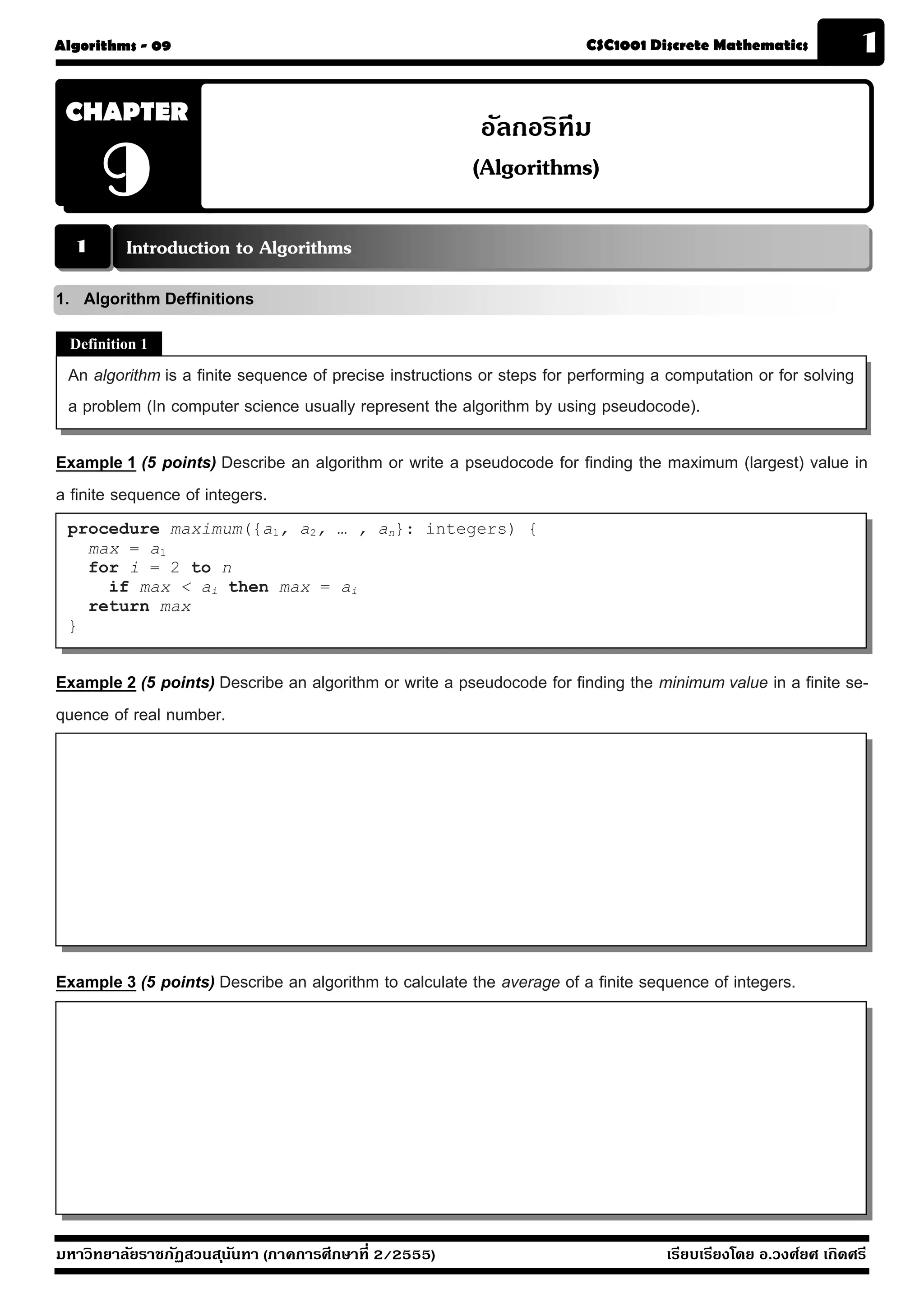
Example 1 (5 points) Describe an algorithm or write a pseudocode for finding the maximum (largest) value in
a finite sequence of integers.
procedure maximum({a1, a2, … , an}: integers) {
max = a1
for i = 2 to n
if max < ai then max = ai
return max
}
Example 2 (5 points) Describe an algorithm or write a pseudocode for finding the minimum value in a finite se-
quence of real number.
Example 3 (5 points) Describe an algorithm to calculate the average of a finite sequence of integers.
มหาวิทยาลัยราชภัฏสวนส ุนันทา (ภาคการศึกษาที่ 2/2555) เรียบเรียงโดย อ.วงศ์ยศ เกิดศรี
2. 2 CSC1001 Discrete Mathematics 09 - Algorithms
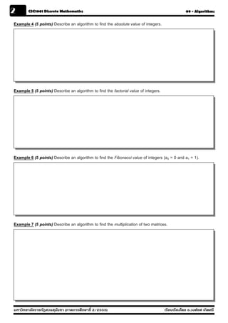
Example 4 (5 points) Describe an algorithm to find the absolute value of integers.
Example 5 (5 points) Describe an algorithm to find the factorial value of integers.
Example 6 (5 points) Describe an algorithm to find the Fibonacci value of integers (a0 = 0 and a1 = 1).
Example 7 (5 points) Describe an algorithm to find the multiplication of two matrices.
มหาวิทยาลัยราชภัฏสวนส ุนันทา (ภาคการศึกษาที่ 2/2555) เรียบเรียงโดย อ.วงศ์ยศ เกิดศรี
3. Algorithms - 09 CSC1001 Discrete Mathematics 3
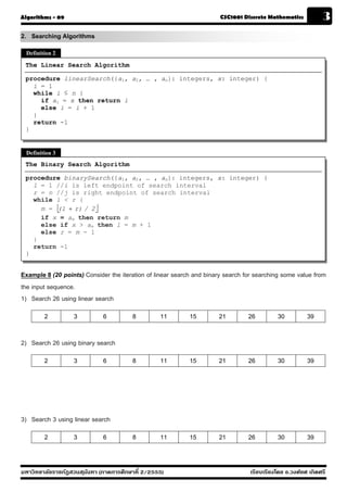
2. Searching Algorithms
Definition 2
The Linear Search Algorithm
procedure linearSearch({a1, a2, … , an}: integers, x: integer) {
i = 1
while i ≤ n {
if ai = x then return i
else i = i + 1
}
return -1
}
Definition 3
The Binary Search Algorithm
procedure binarySearch({a1, a2, … , an}: integers, x: integer) {
l = 1 //i is left endpoint of search interval
r = n //j is right endpoint of search interval
while l < r {
m = ⎣ + r) / 2 ⎦
(l
if x = am then return m
else if x > am then l = m + 1
else r = m - 1
}
return -1
}
Example 8 (20 points) Consider the iteration of linear search and binary search for searching some value from
the input sequence.
1) Search 26 using linear search
2 3 6 8 11 15 21 26 30 39
2) Search 26 using binary search
2 3 6 8 11 15 21 26 30 39
3) Search 3 using linear search
2 3 6 8 11 15 21 26 30 39
มหาวิทยาลัยราชภัฏสวนส ุนันทา (ภาคการศึกษาที่ 2/2555) เรียบเรียงโดย อ.วงศ์ยศ เกิดศรี
4. 4 CSC1001 Discrete Mathematics 09 - Algorithms
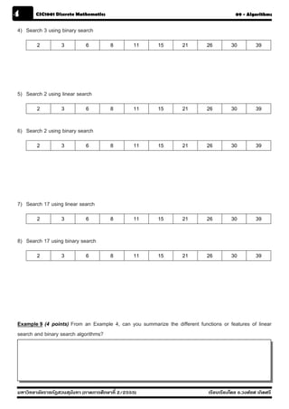
4) Search 3 using binary search
2 3 6 8 11 15 21 26 30 39
5) Search 2 using linear search
2 3 6 8 11 15 21 26 30 39
6) Search 2 using binary search
2 3 6 8 11 15 21 26 30 39
7) Search 17 using linear search
2 3 6 8 11 15 21 26 30 39
8) Search 17 using binary search
2 3 6 8 11 15 21 26 30 39
Example 9 (4 points) From an Example 4, can you summarize the different functions or features of linear
search and binary search algorithms?
มหาวิทยาลัยราชภัฏสวนส ุนันทา (ภาคการศึกษาที่ 2/2555) เรียบเรียงโดย อ.วงศ์ยศ เกิดศรี
5. Algorithms - 09 CSC1001 Discrete Mathematics 5
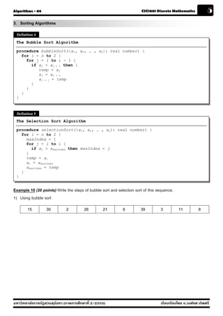
3. Sorting Algorithms
Definition 4
The Bubble Sort Algorithm
procedure bubbleSort({a1, a2, … , an}: real number) {
for i = n to 2 {
for j = 1 to i - 1 {
if aj > aj + 1 then {
temp = aj
aj = aj + 1
aj + 1 = temp
}
}
}
}
Definition 5
The Selection Sort Algorithm
procedure selectionSort({a1, a2, … , an}: real number) {
for i = n to 2 {
maxIndex = 1
for j = 1 to i {
if aj > amaxIndex then maxIndex = j
}
temp = ai
ai = amaxIndex
amaxIndex = temp
}
}
Example 10 (20 points) Write the steps of bubble sort and selection sort of this sequence.
1) Using bubble sort
15 30 2 26 21 6 39 3 11 8
มหาวิทยาลัยราชภัฏสวนส ุนันทา (ภาคการศึกษาที่ 2/2555) เรียบเรียงโดย อ.วงศ์ยศ เกิดศรี
6. 6 CSC1001 Discrete Mathematics 09 - Algorithms
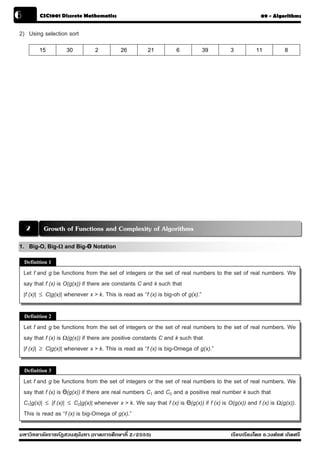
2) Using selection sort
15 30 2 26 21 6 39 3 11 8
2 Growth of Functions and Complexity of Algorithms
1. Big-O, Big-Ω and Big-Θ Notation
Definition 1
Let f and g be functions from the set of integers or the set of real numbers to the set of real numbers. We
say that f (x) is O(g(x)) if there are constants C and k such that
|f (x)| ≤ C|g(x)| whenever x > k. This is read as “f (x) is big-oh of g(x).”
Definition 2
Let f and g be functions from the set of integers or the set of real numbers to the set of real numbers. We
say that f (x) is Ω(g(x)) if there are positive constants C and k such that
|f (x)| ≥ C|g(x)| whenever x > k. This is read as “f (x) is big-Omega of g(x).”
Definition 3
Let f and g be functions from the set of integers or the set of real numbers to the set of real numbers. We
say that f (x) is Θ(g(x)) if there are real numbers C1 and C2 and a positive real number k such that
C1|g(x)| ≤ |f (x)| ≤ C2|g(x)| whenever x > k. We say that f (x) is Θ(g(x)) if f (x) is O(g(x)) and f (x) is Ω(g(x)).
This is read as “f (x) is big-Omega of g(x).”
มหาวิทยาลัยราชภัฏสวนส ุนันทา (ภาคการศึกษาที่ 2/2555) เรียบเรียงโดย อ.วงศ์ยศ เกิดศรี
7. Algorithms - 09 CSC1001 Discrete Mathematics 7
Example 11 (4 points) Show that f(x) = x2 + 2x + 1 is O(x2).
Example 12 (4 points) Show that f(x) = 3x4 + 5x2 + 15 is O(x4).
Example 13 (4 points) Show that f(x) = 7x2 is O(x3) by replace x into f(x).
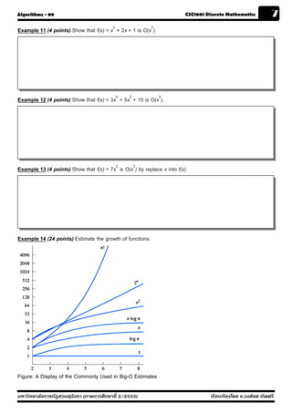
Example 14 (24 points) Estimate the growth of functions.
Figure: A Display of the Commonly Used in Big-O Estimates
มหาวิทยาลัยราชภัฏสวนส ุนันทา (ภาคการศึกษาที่ 2/2555) เรียบเรียงโดย อ.วงศ์ยศ เกิดศรี
8. 8 CSC1001 Discrete Mathematics 09 - Algorithms
1) (12 points) Ranking the speed rate of functions by descending
No Functions Ranking No Functions Ranking
1. n 7. n2
2. 0.5n 8. log6 n
3. n log n 9. n0.5
4. 1 10. n!
5. n2 log n 11. 2n
6. log n 12. n3
2) (12 points) Ranking the growth rate of functions by descending
No Functions Ranking No Functions Ranking
1. n 7. n2
2. 0.5n 8. log6 n
3. n log n 9. n0.5
4. 1 10. n!
5. n2 log n 11. 2n
6. log n 12. n3
Example 15 (4 points) Show that f(x) = 5x3 + 2x2 - 4x + 1 is Ω(x4).
Example 16 (4 points) Show that 3x2 + 8x log x is Θ(x2).
มหาวิทยาลัยราชภัฏสวนส ุนันทา (ภาคการศึกษาที่ 2/2555) เรียบเรียงโดย อ.วงศ์ยศ เกิดศรี
9. Algorithms - 09 CSC1001 Discrete Mathematics 9
Example 17 (4 points) Find Big-O of f(x) + g(x) if f(x) = 4x5 + 2x – 10 and g(x) = x3 log x + 10x
2. Time Complexity of Algorithms
The time complexity of an algorithm can be expressed in terms of the number of operations used by the
algorithm when the input has a particular size. The operations used to measure time complexity can be the
comparison of integers, the addition of integers, the multiplication of integers, the division of integers, or any
other basic operation.
Example 18 (5 points) Analyze the time complexity of Finding maximum value algorithm.
procedure maximum({a1, a2, … , an}: integers) {
max = a1
for i = 2 to n
if max < ai then max = ai
return max
}
Example 19 (5 points) Analyze the time complexity of an algorithm in Example 3.
มหาวิทยาลัยราชภัฏสวนส ุนันทา (ภาคการศึกษาที่ 2/2555) เรียบเรียงโดย อ.วงศ์ยศ เกิดศรี
10. 10 CSC1001 Discrete Mathematics 09 - Algorithms
Example 20 (5 points) Analyze the time complexity of an algorithm in Example 4.
Example 21 (5 points) Analyze the time complexity of an algorithm in Example 5.
Example 22 (5 points) Analyze the time complexity of an algorithm in Example 6.
Example 23 (5 points) Analyze the time complexity of an algorithm in Example 7.
มหาวิทยาลัยราชภัฏสวนส ุนันทา (ภาคการศึกษาที่ 2/2555) เรียบเรียงโดย อ.วงศ์ยศ เกิดศรี
11. Algorithms - 09 CSC1001 Discrete Mathematics 11
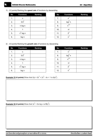
Example 24 (13 points) Find the Big-O notation of a part of Java program.
No. A Part of Java Program Big-O
int temp = a[i];
1. a[i] = a[a.length - i - 1];
a[a.length - i - 1] = temp;
for (int i = a.length - 1; i >= 0; i--) {
if (a[i] == x) {
2. System.out.println(i);
}
}
for (int i = 0; i <= n; i = i + 4) {
3. System.out.println(a[i]);
}
for (int i = 0; i < a.length; i++) {
for (int j = 0; j < a[i].length; j++) {
4. a[i][j] = 13;
}
}
for (int i = 10000000; i >= 2; i--) {
System.out.println(a[i]);
5. System.out.println(a[i - 1]);
System.out.println(a[i - 2]);
}
for (int i = 0; i < n; i++) {
for (int j = i; j >= 0; j--) {
System.out.print(a[i][j] + " ");
6. }
System.out.println();
}
for (int i = 0; i < n; i++) {
for (int j = 100; j >= 0; j--) {
System.out.print(a[i][j] + " ");
7. }
System.out.print("----------------");
System.out.println();
}
for (int i = 0; i <= n; i = i * 2) {
8. System.out.println(a[i]);
}
for (int i = 0; i < n; i++) {
for (int j = n; j >= 0; j = j / 5) {
System.out.print(a[i][j]);
9. System.out.println();
}
}
for (int i = 0; i < n; i += 100) {
for (int j = 0; j <= 200; j++) {
System.out.print(a[i][j] + " ");
sum = sum + a[i][j];
10. }
}
for (int i = 0; i <= n; i = i * 2) {
System.out.println(b[i]);
}
มหาวิทยาลัยราชภัฏสวนส ุนันทา (ภาคการศึกษาที่ 2/2555) เรียบเรียงโดย อ.วงศ์ยศ เกิดศรี
12. 12 CSC1001 Discrete Mathematics 09 - Algorithms
No. A Part of Java Program Big-O
for (int i = 0; i < mul.length; i++) {
for (int j = 0; j < mul[i].length; j++) {
for (int k = 0; k < y.length; k++) {
11. mul[i][j] += x[i][k] * y[k][j];
}
}
}
for (int i = 0; i < n; i++) {
for (int j = i; j >= 0; j -= 2) {
for (int k = 0; k < n; k *= 10) {
12. mul[i][j] += x[i][k] * y[k][j];
}
}
}
int left = 0, right = n, index = -1;
while (left <= right) {
int mid = (left + right) / 2;
13. if (key == a[mid]) index = mid;
else if (key < a[mid]) right = mid - 1;
else left = mid + 1;
}
มหาวิทยาลัยราชภัฏสวนส ุนันทา (ภาคการศึกษาที่ 2/2555) เรียบเรียงโดย อ.วงศ์ยศ เกิดศรี