Download as PDF, PPTX


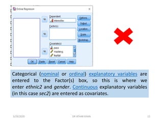
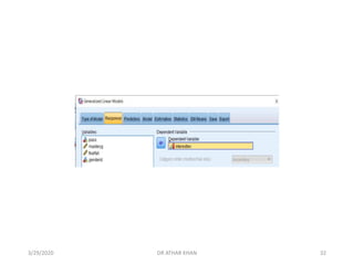
![Here, we place “Interestlev” variable in the dependent box and remaining
variables (IV’s) in the Covariate(s) box. Although they are categorical variables,
we can include “pass” and “genderid" as covariates.
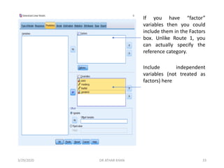
However, if you have categorical variables with more than two levels, then you
must use the “factor(s)” box for them. [FYI, would have also entered the
above variables as factors, but I prefer having control over the designation of
the reference category; SPSS defaults by treating the category with the
higher value as the reference category]
3/29/2020 DR ATHAR KHAN 11](https://image.slidesharecdn.com/ordinallogisticregression-converted-200329155907/85/Ordinal-logistic-regression-11-320.jpg)
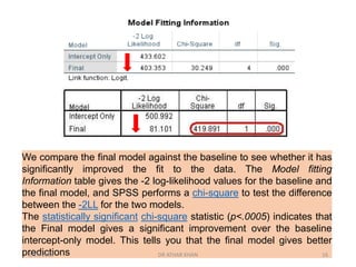
![The Model Fitting Information (see right) contains the -2 Log
Likelihood for:
Intercept only (or null) model and the Full Model
(containing the full set of predictors).
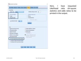
We also have a likelihood ratio chi-square test to test
whether there is a significant improvement in fit of the Final
model relative to the Intercept only model.
In this case, we see a significant improvement in fit of the
Final model over the null model [χ²(4)=30.249, p<.001].
3/29/2020 DR ATHAR KHAN 15](https://image.slidesharecdn.com/ordinallogisticregression-converted-200329155907/85/Ordinal-logistic-regression-15-320.jpg)
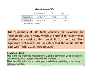
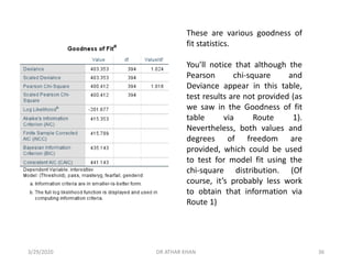
![In this analysis, we see that both the Pearson chi-square test
[χ²(394)=400.412, p=.401] and the deviance test
[χ²(394)=403.353, p=.362] were both non-significant. These
results suggest good model fit.
3/29/2020 DR ATHAR KHAN 18](https://image.slidesharecdn.com/ordinallogisticregression-converted-200329155907/85/Ordinal-logistic-regression-18-320.jpg)
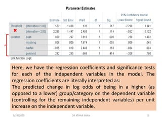
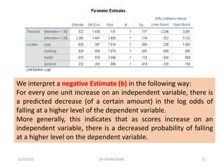
![Fear of failure was not a significant predictor in the model. [The
coefficient is interpreted as follows: For every one unit increase
on fear of failure, there is a predicted decrease of .015 in the
log odds of being in a higher level of the dependent variable.]
“Fearfail” is fear of failure (higher scores indicate greater fear of failure).
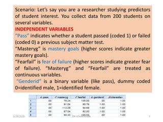
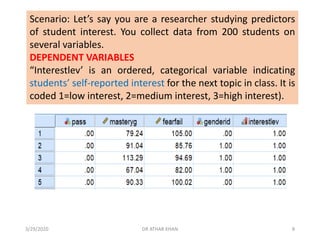
“Interestlev’ is an ordered, categorical variable indicating students’ self-
reported interest for the next topic in class. It is coded 1=low interest,
2=medium interest, 3=high interest).
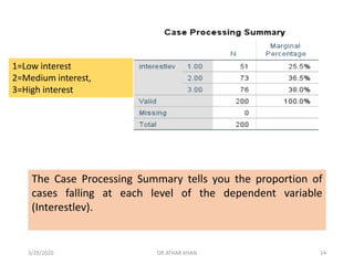
3/29/2020 DR ATHAR KHAN 23](https://image.slidesharecdn.com/ordinallogisticregression-converted-200329155907/85/Ordinal-logistic-regression-23-320.jpg)
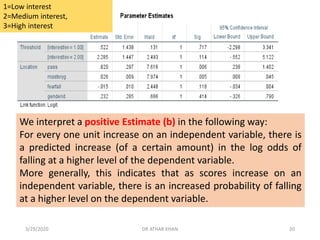
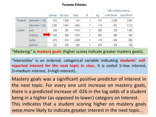
![Gender identification was not a significant predictor. [Again,
because this is a binary variable the slope can be thought of as
the difference in log odds between groups. On average, the log
odds of being in a higher Interest category was .232 points
greater for persons identified as female than males.]
“Genderid” is a binary variable (like pass), dummy coded 0=identified male,
1=identified female.
“Interestlev’ is an ordered, categorical variable indicating students’ self-
reported interest for the next topic in class. It is coded 1=low interest,
2=medium interest, 3=high interest).
3/29/2020 DR ATHAR KHAN 25](https://image.slidesharecdn.com/ordinallogisticregression-converted-200329155907/85/Ordinal-logistic-regression-25-320.jpg)

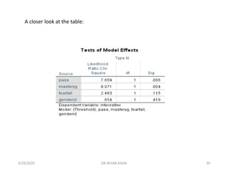
![This is the Likelihood ratio chi-square
test we saw via Route 1. We see that
our full model was a significant
improvement in fit over the null (no
predictors) model [χ²(4)=30.249,
p<.001].
3/29/2020 DR ATHAR KHAN 37](https://image.slidesharecdn.com/ordinallogisticregression-converted-200329155907/85/Ordinal-logistic-regression-37-320.jpg)
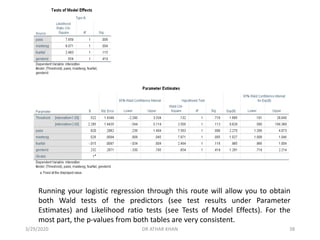
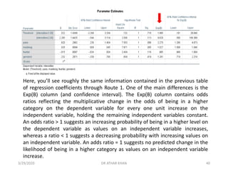
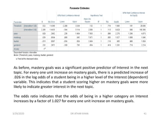
![Fear of failure was not a significant predictor in the model. [The regression
coefficient indicates that for every one unit increase on fear of failure, there is a
predicted decrease of .015 in the log odds of being in a higher level of the
dependent variable (controlling for the remaining predictors).]
The odds ratio indicates that the odds of being in a higher category on Interest
increases by a factor of .985 for every one unit increase on fear of failure. [Given
that the odds ratio is < 1, this indicates a decreasing probability of being in a higher
level on the Interest variable as scores increase on fear of failure.]
3/29/2020 DR ATHAR KHAN 42](https://image.slidesharecdn.com/ordinallogisticregression-converted-200329155907/85/Ordinal-logistic-regression-42-320.jpg)
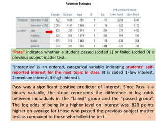
![▪ Pass was a significant positive predictor of Interest. The log odds of being in a
higher level on Interest was .820 points higher on average for those who passed
the previous subject matter test than those who failed the test.
▪ The odds of students who passed (the previous subject matter test) being in a
higher category on the dependent variable were 2.270 times that of those who
failed the test.
▪ Gender identification was not a significant predictor. [On average, the log odds of
being in a higher Interest category was .232 points greater for females than
males.]
▪ The odds of a student identified as female being in a higher category on the
dependent variable was 1.261 times that of a student identified as male (although
again, gender identification was not a significant predictor).
3/29/2020 DR ATHAR KHAN 43](https://image.slidesharecdn.com/ordinallogisticregression-converted-200329155907/85/Ordinal-logistic-regression-43-320.jpg)

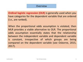
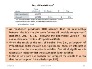
This document provides an overview of ordinal logistic regression (OLR). OLR is used when the dependent variable has ordered categories and the proportional odds assumption is met. Violations of this assumption indicate multinomial logistic regression may be a better alternative. The document discusses key aspects of OLR including interpretation of regression coefficients and odds ratios. It also provides an example analyzing predictors of student interest, finding mastery goals and passing a previous test significantly increased odds of higher interest while fear of failure decreased odds.