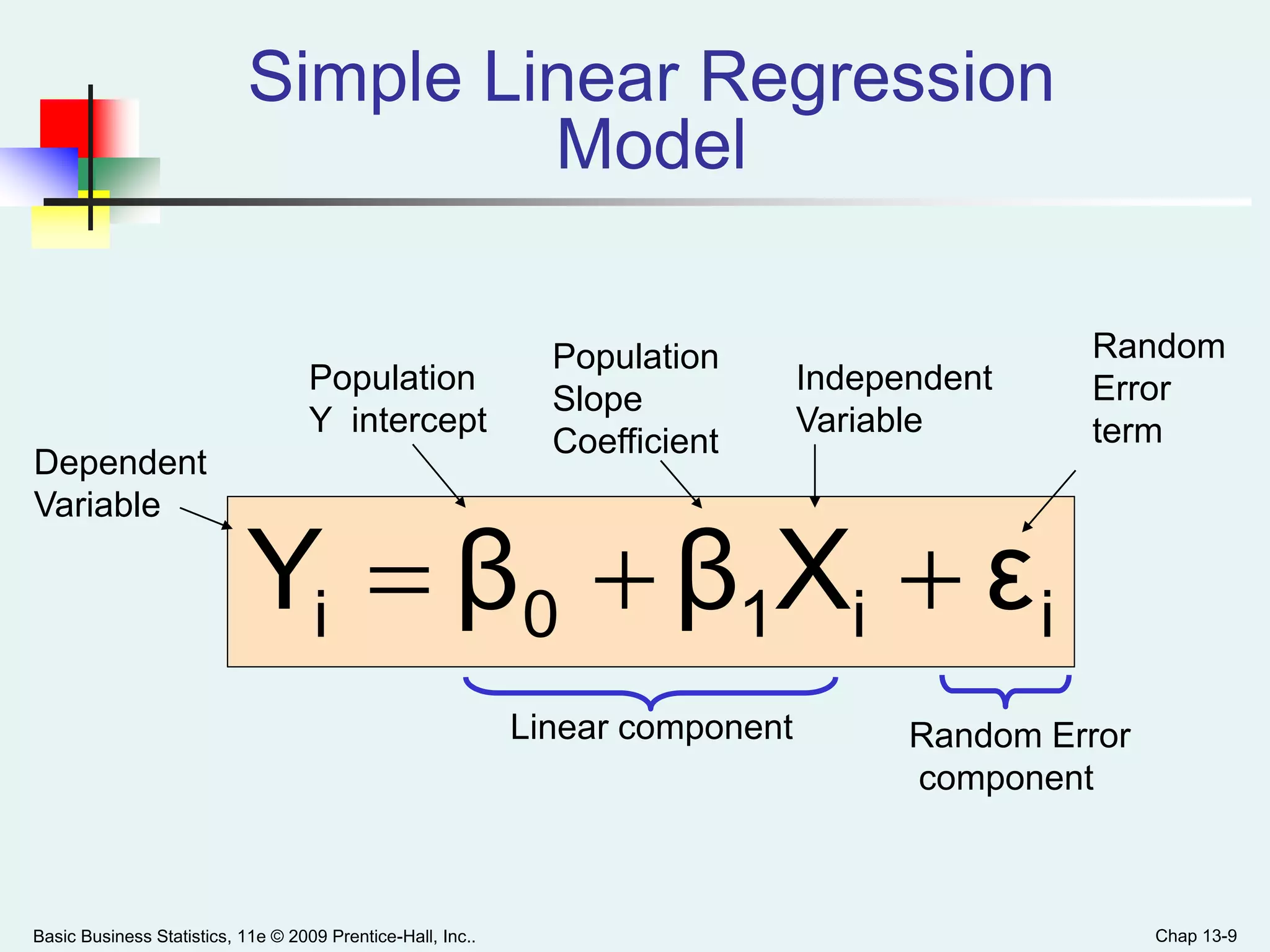
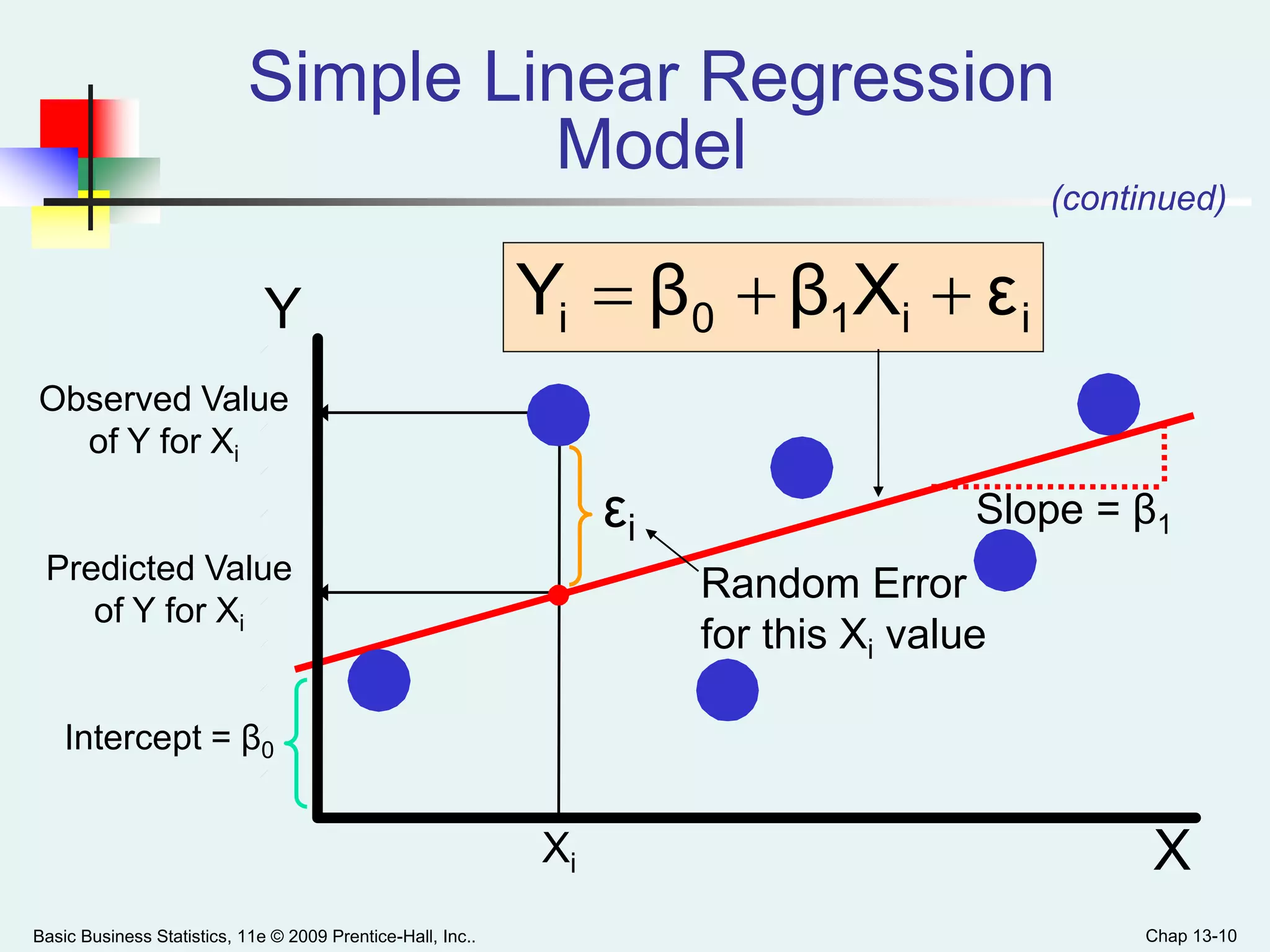
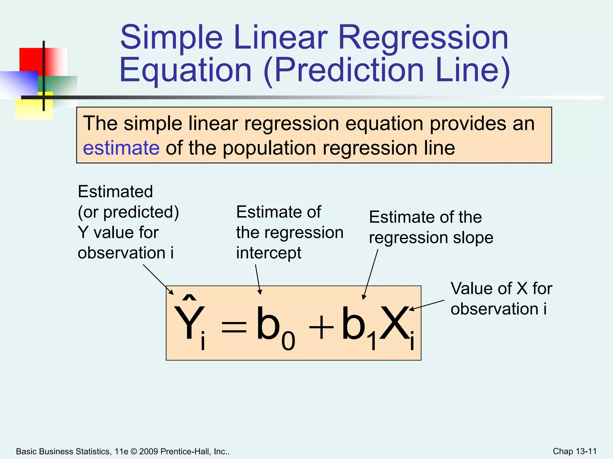
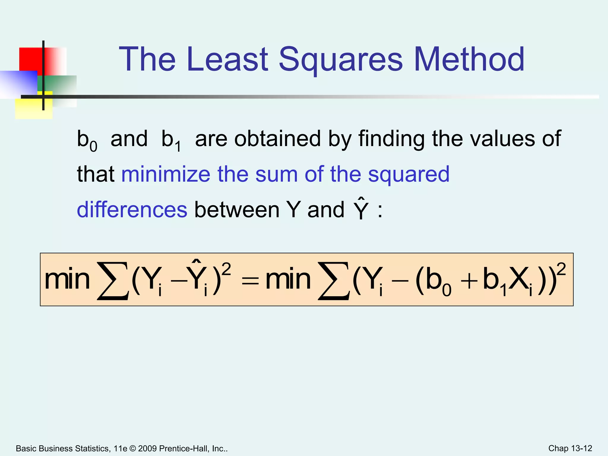
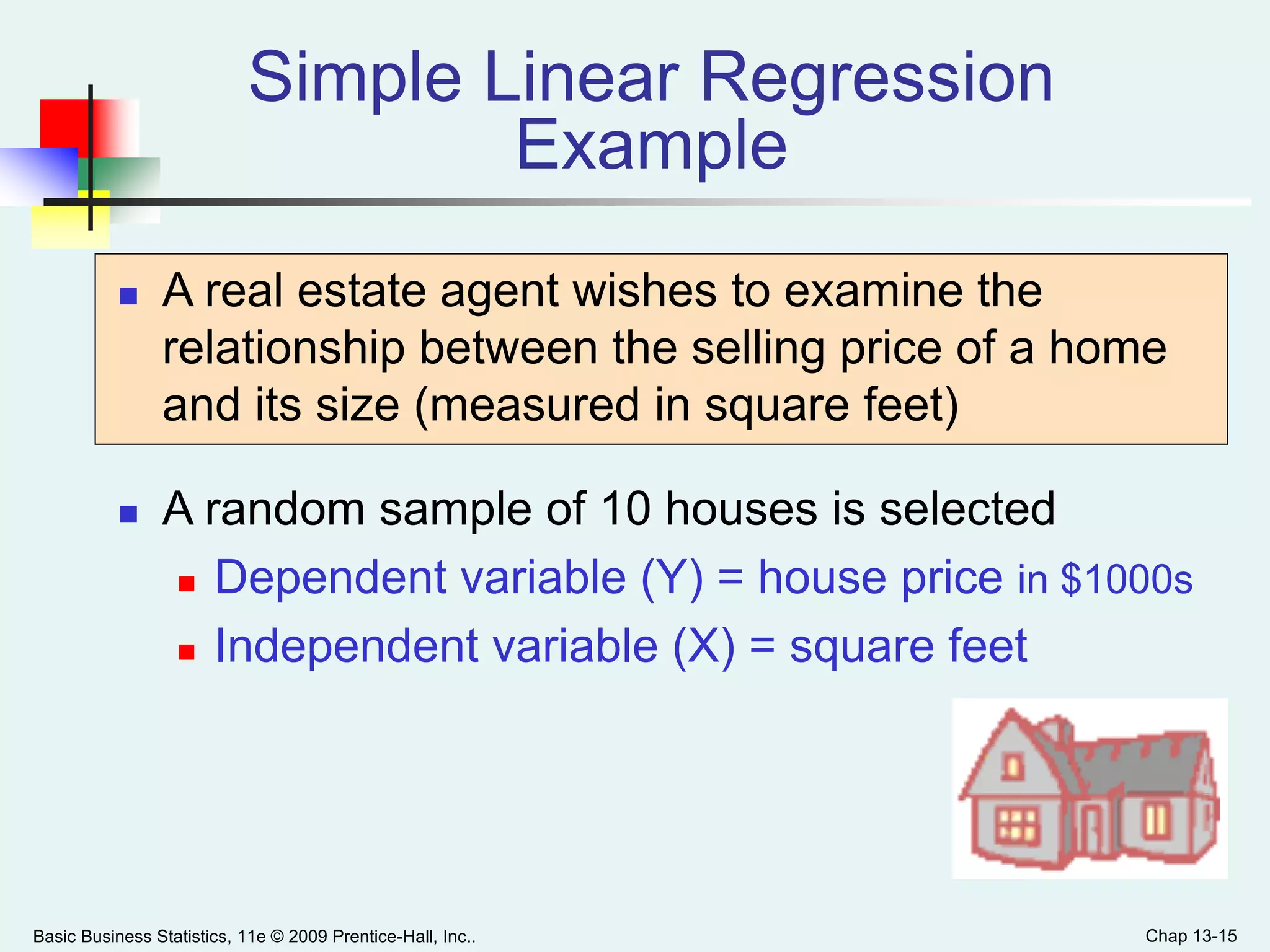
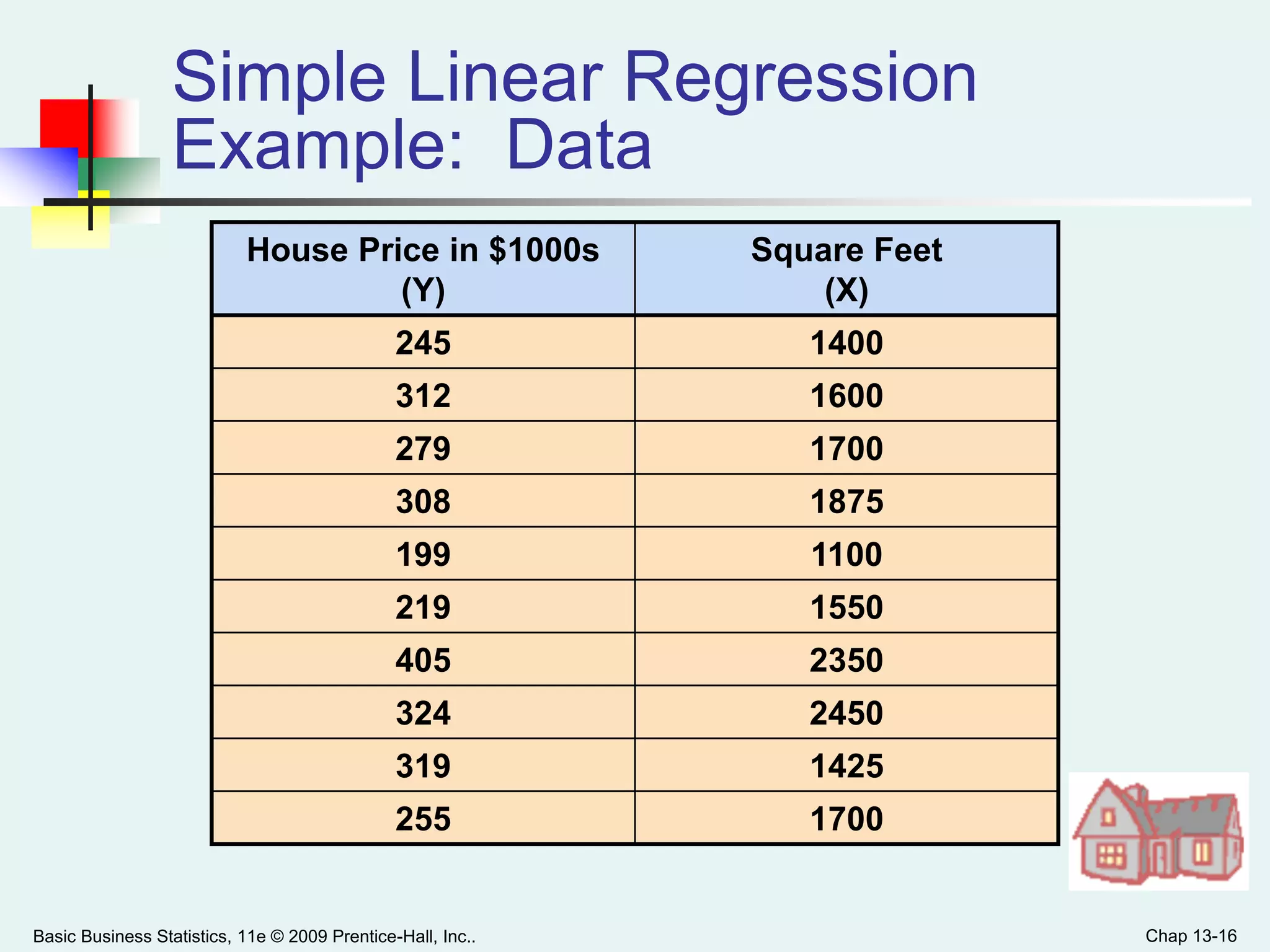
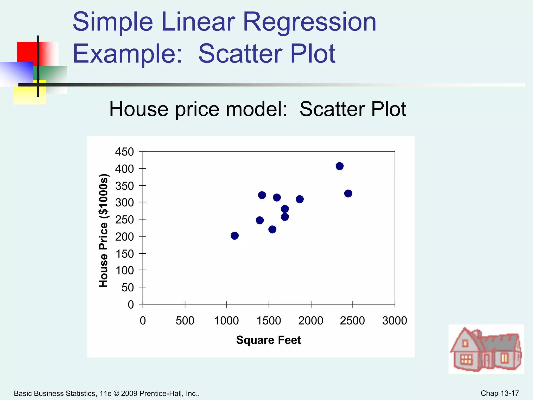
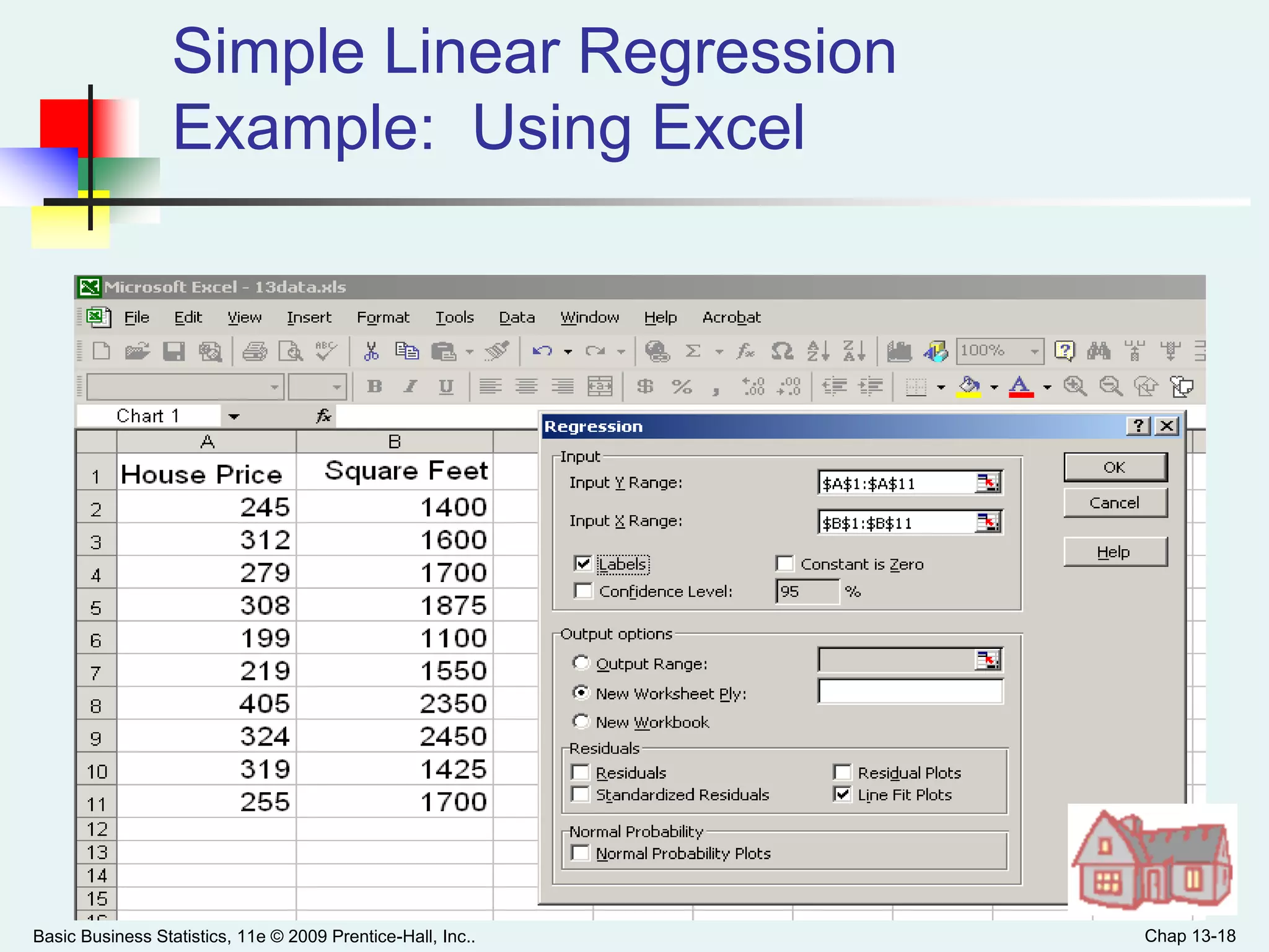
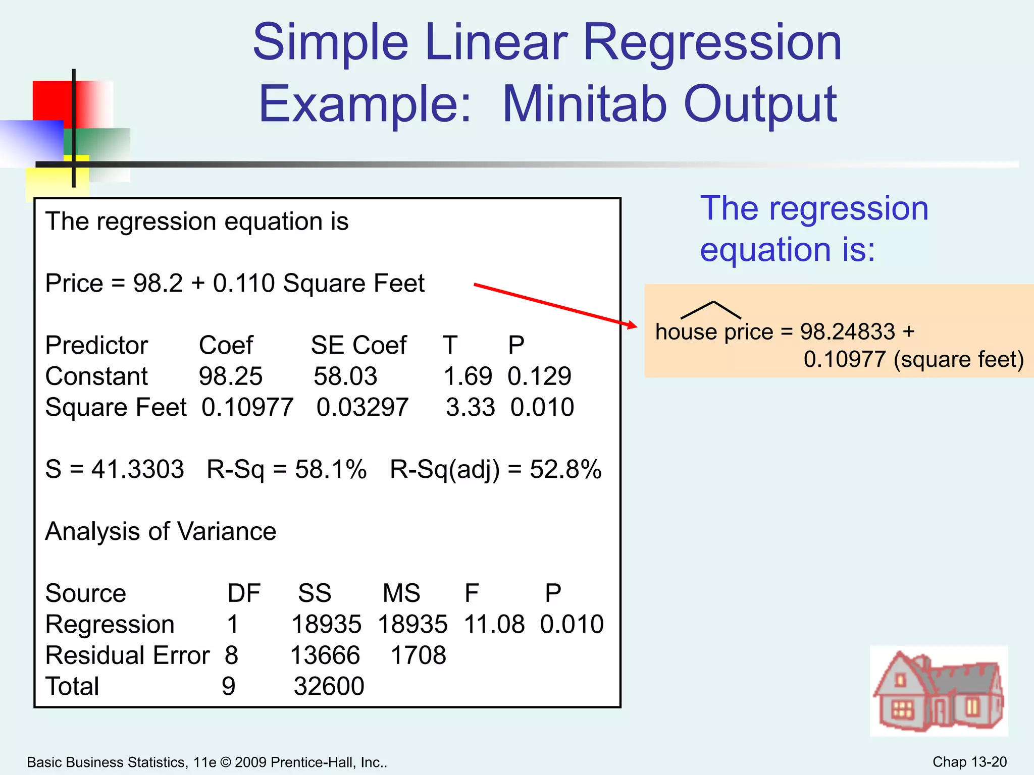
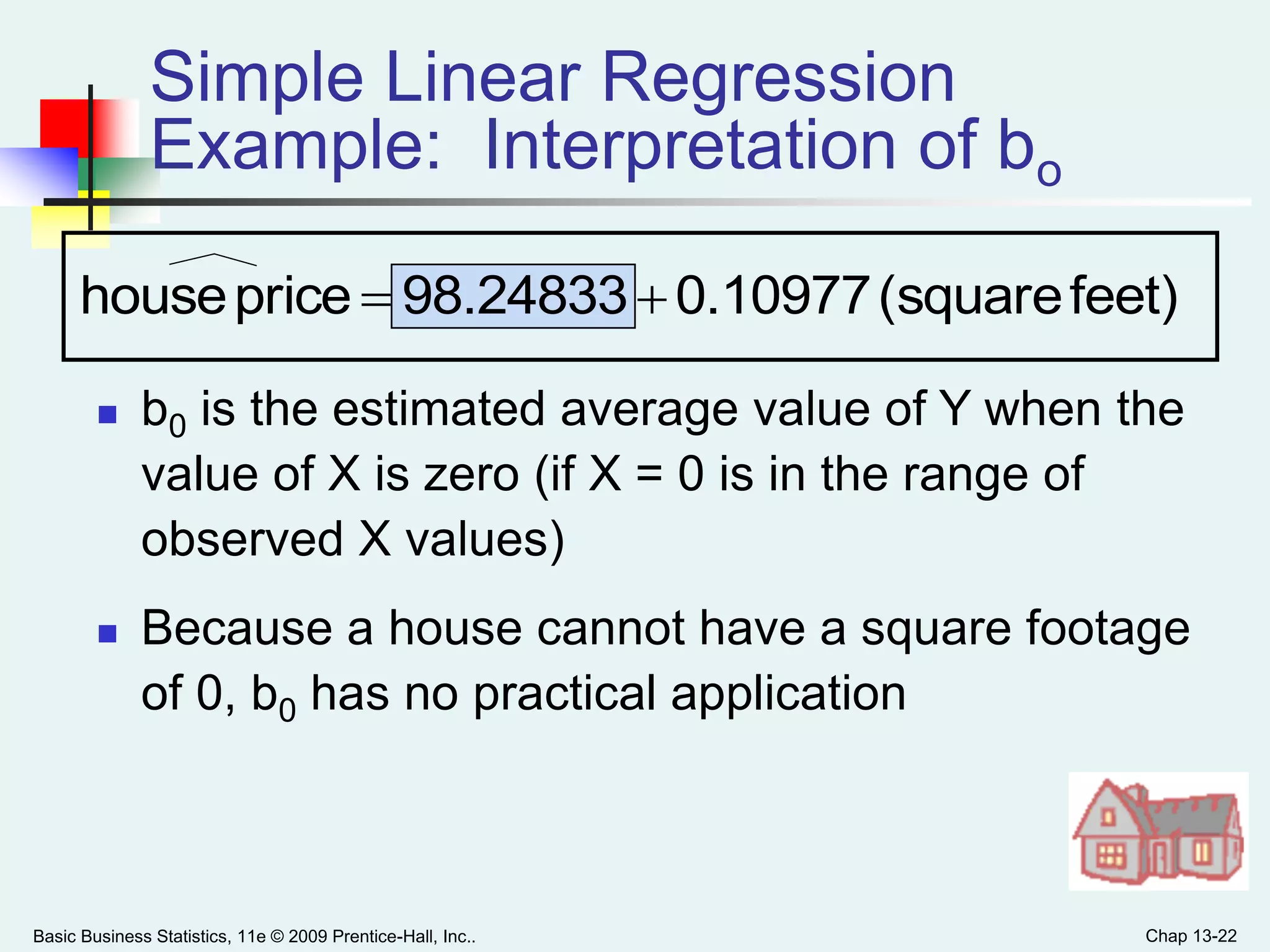
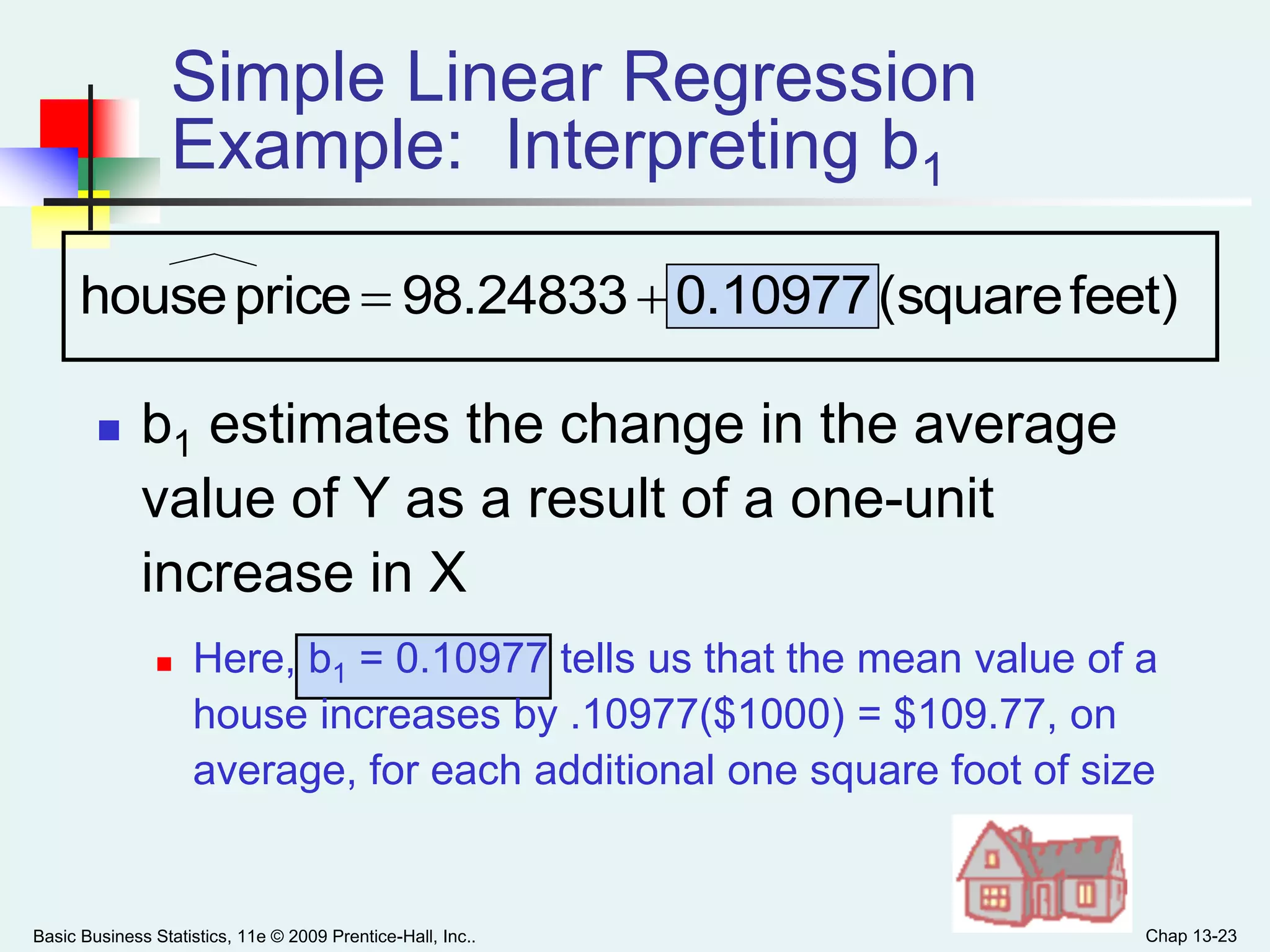
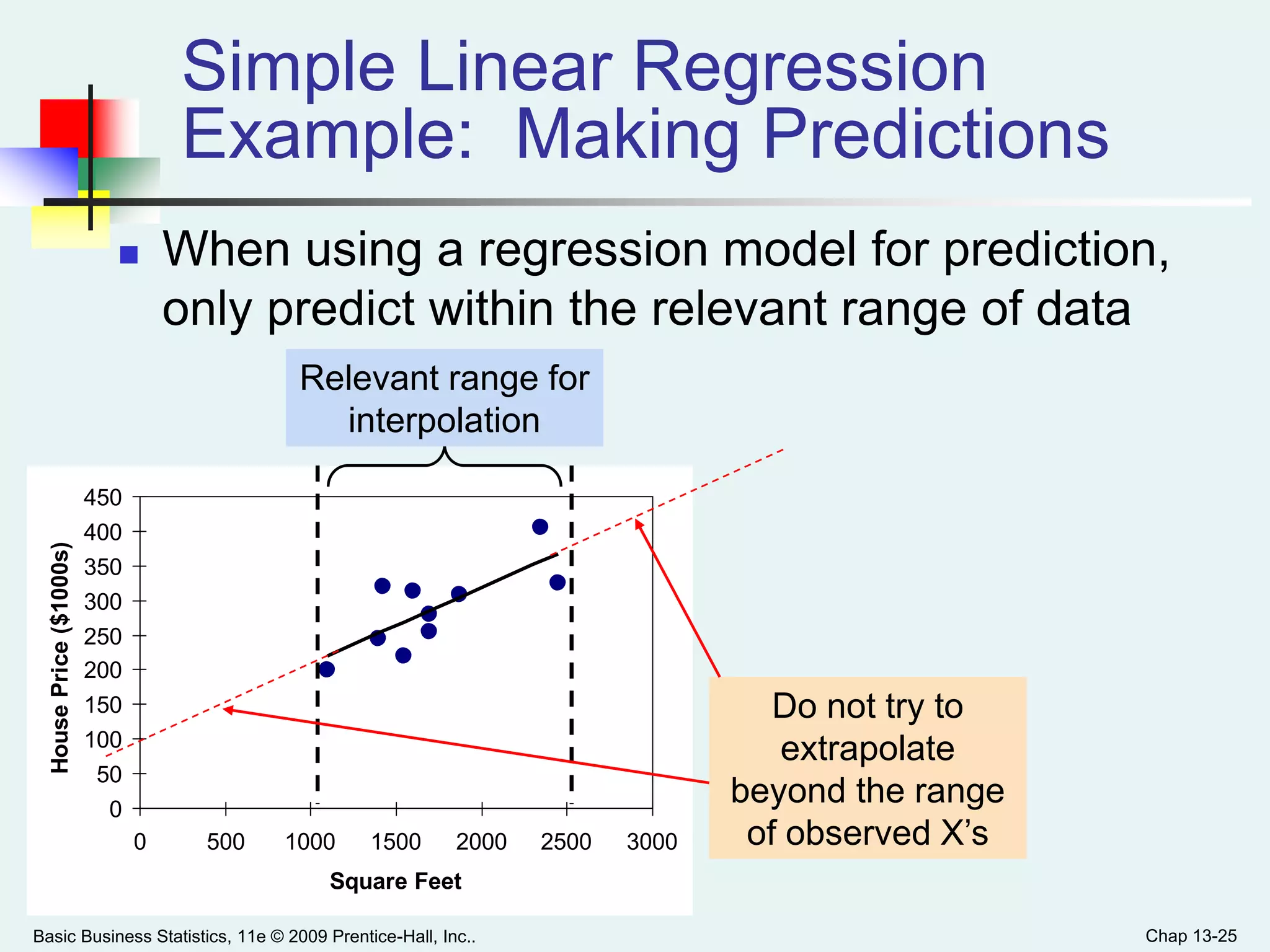
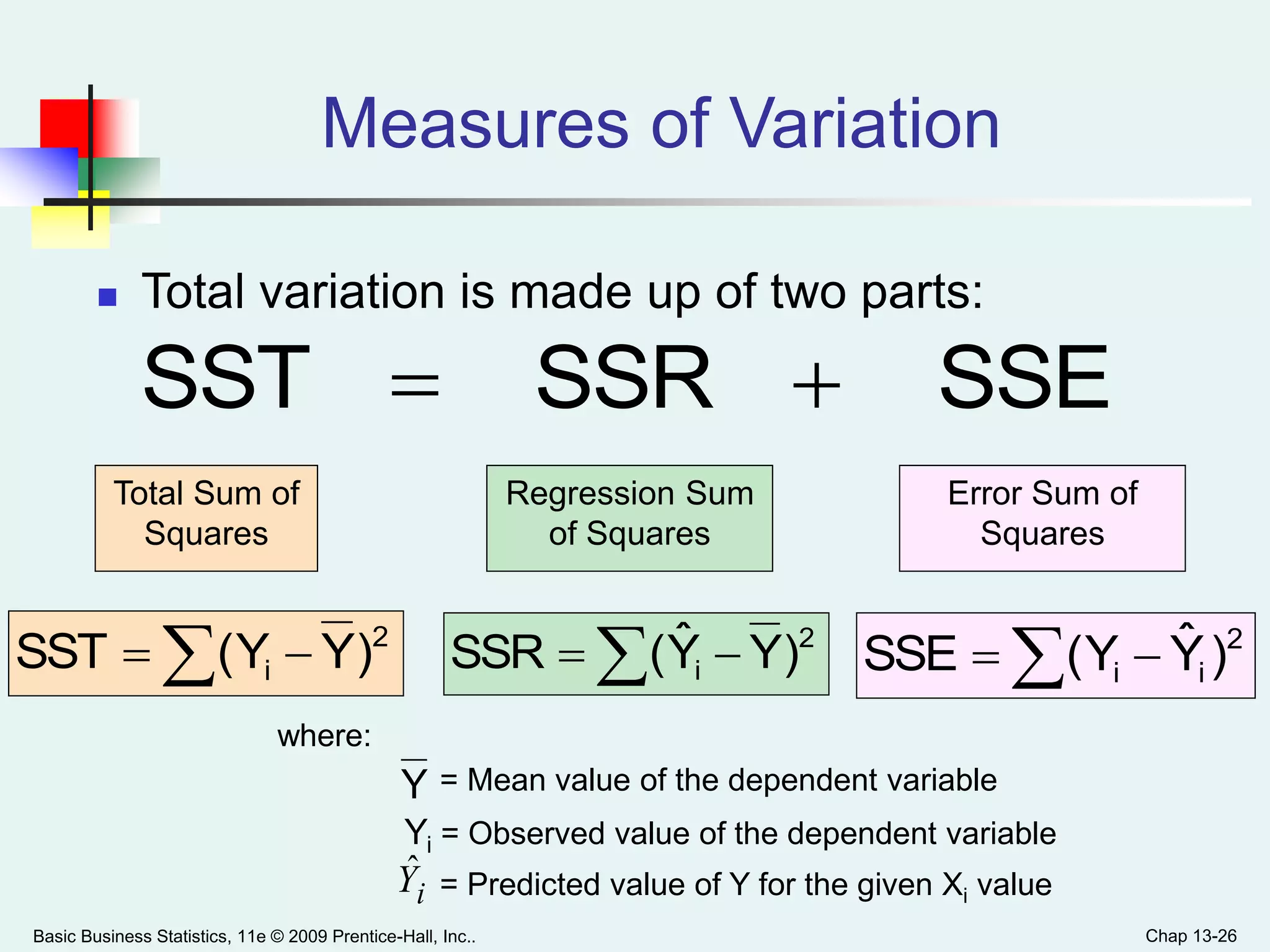
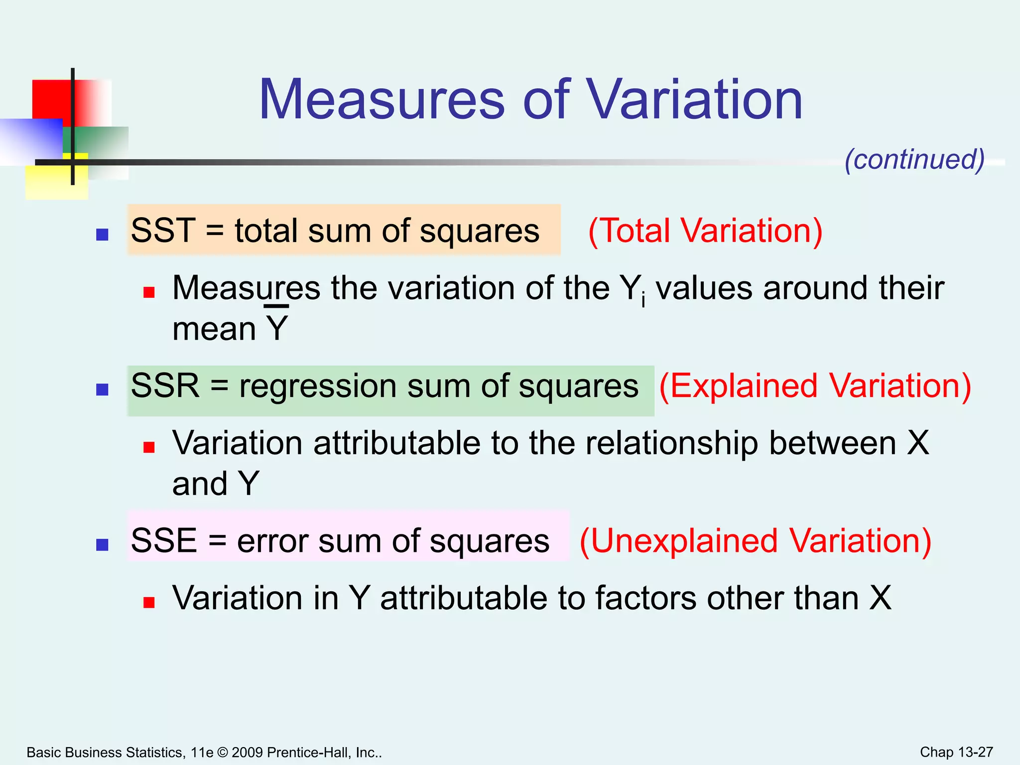
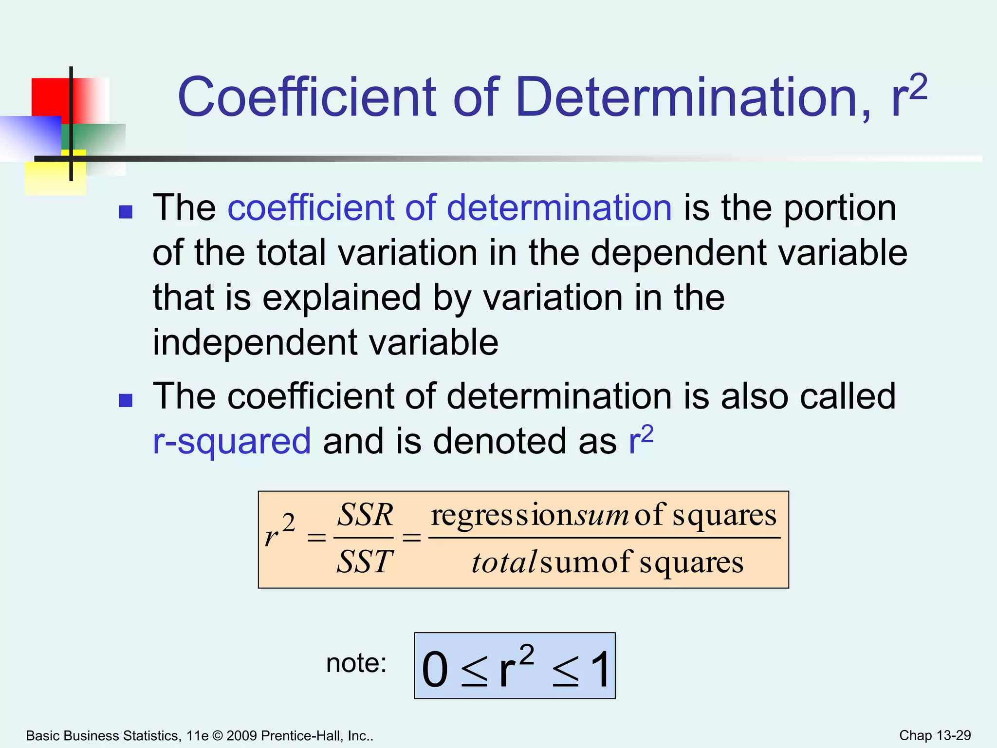
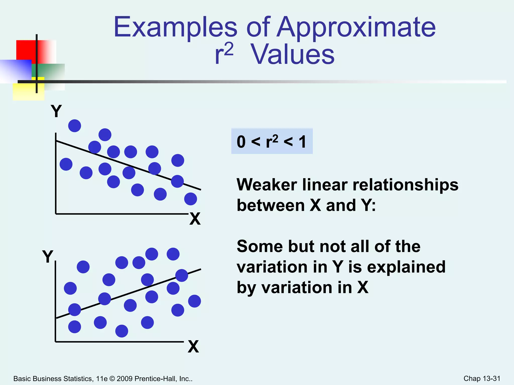
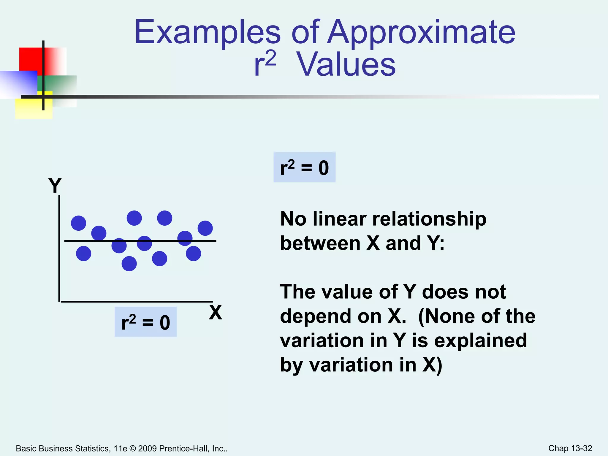
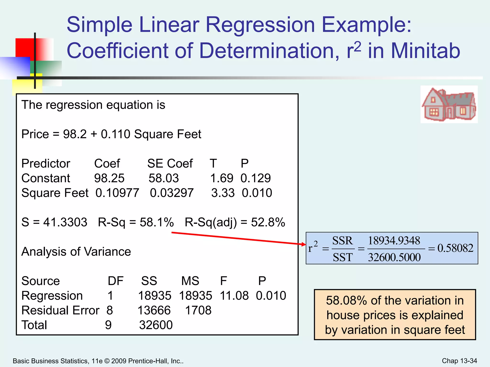
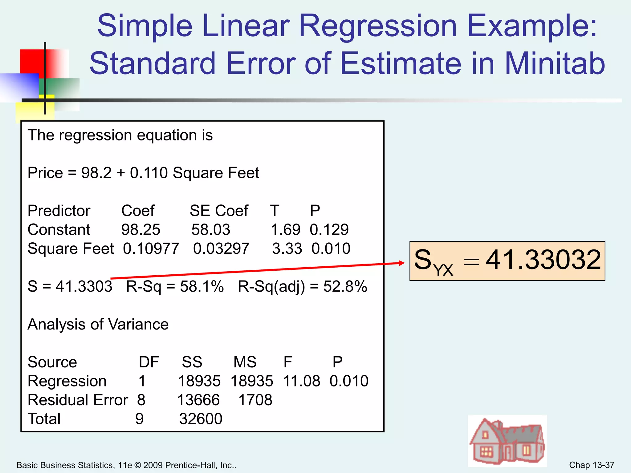
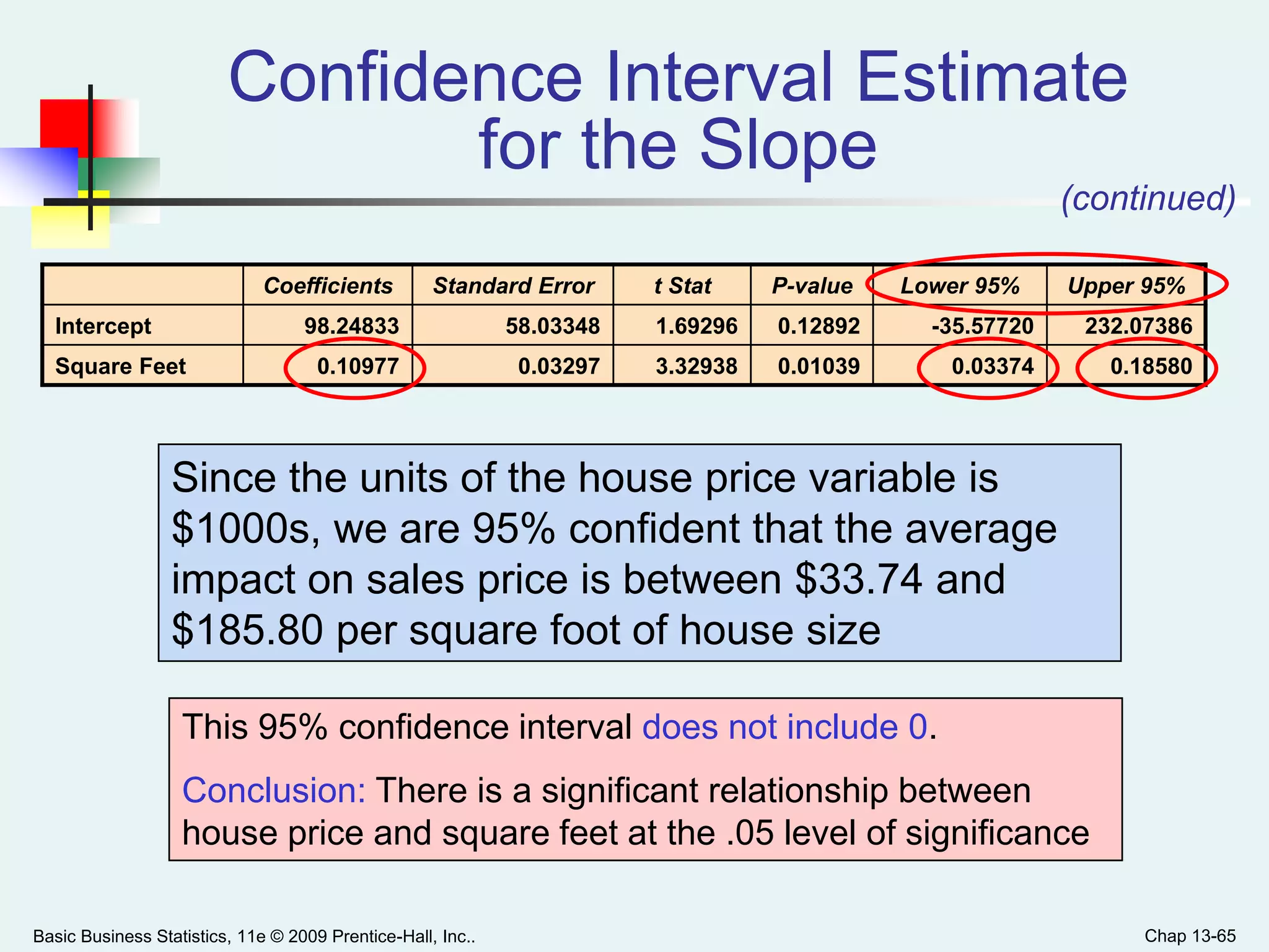
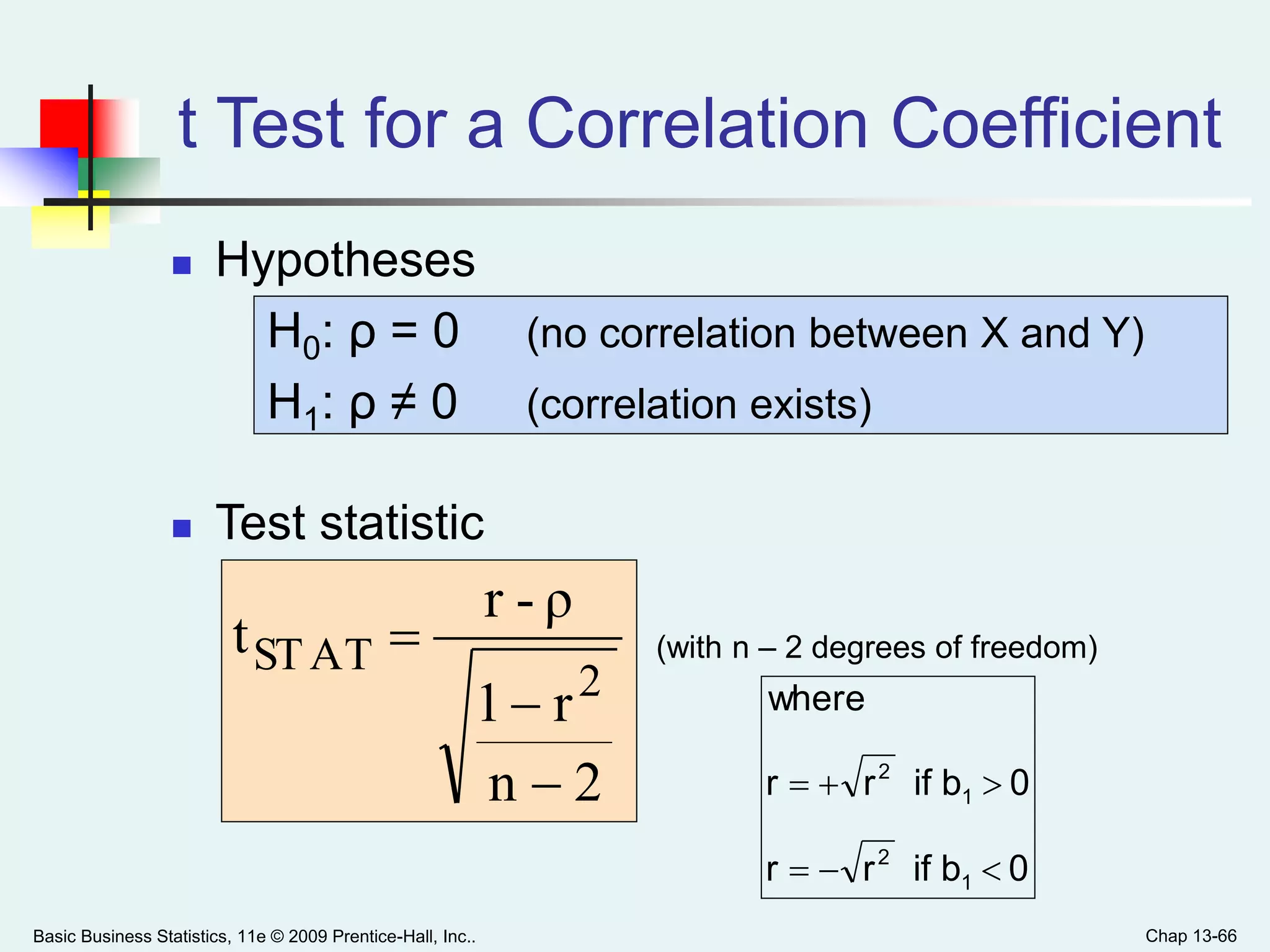
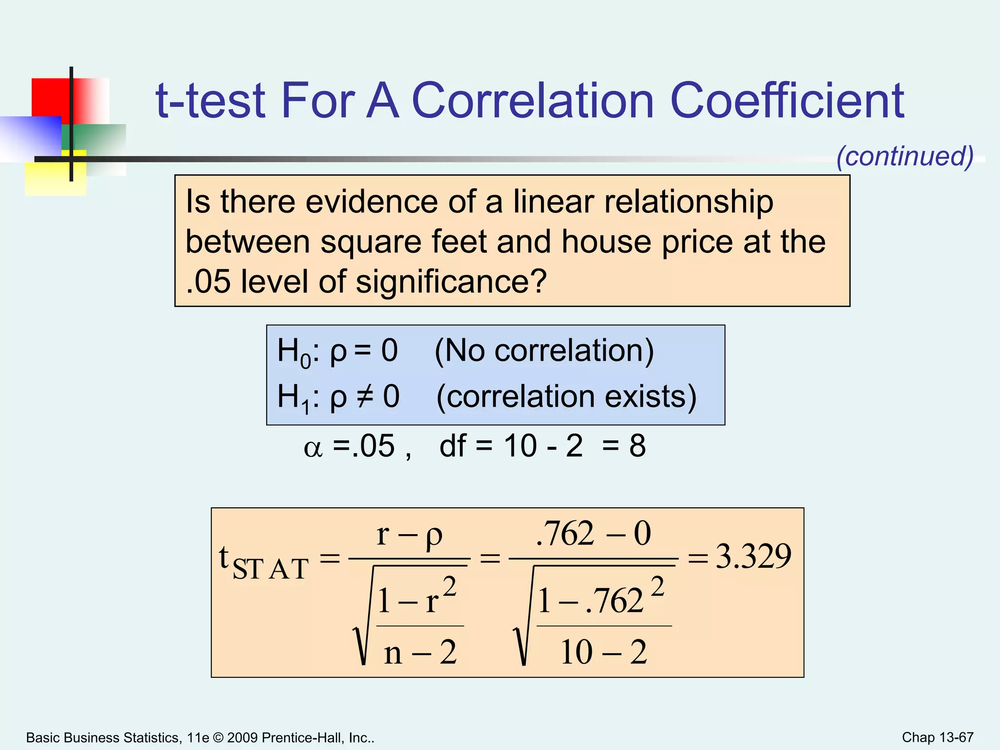
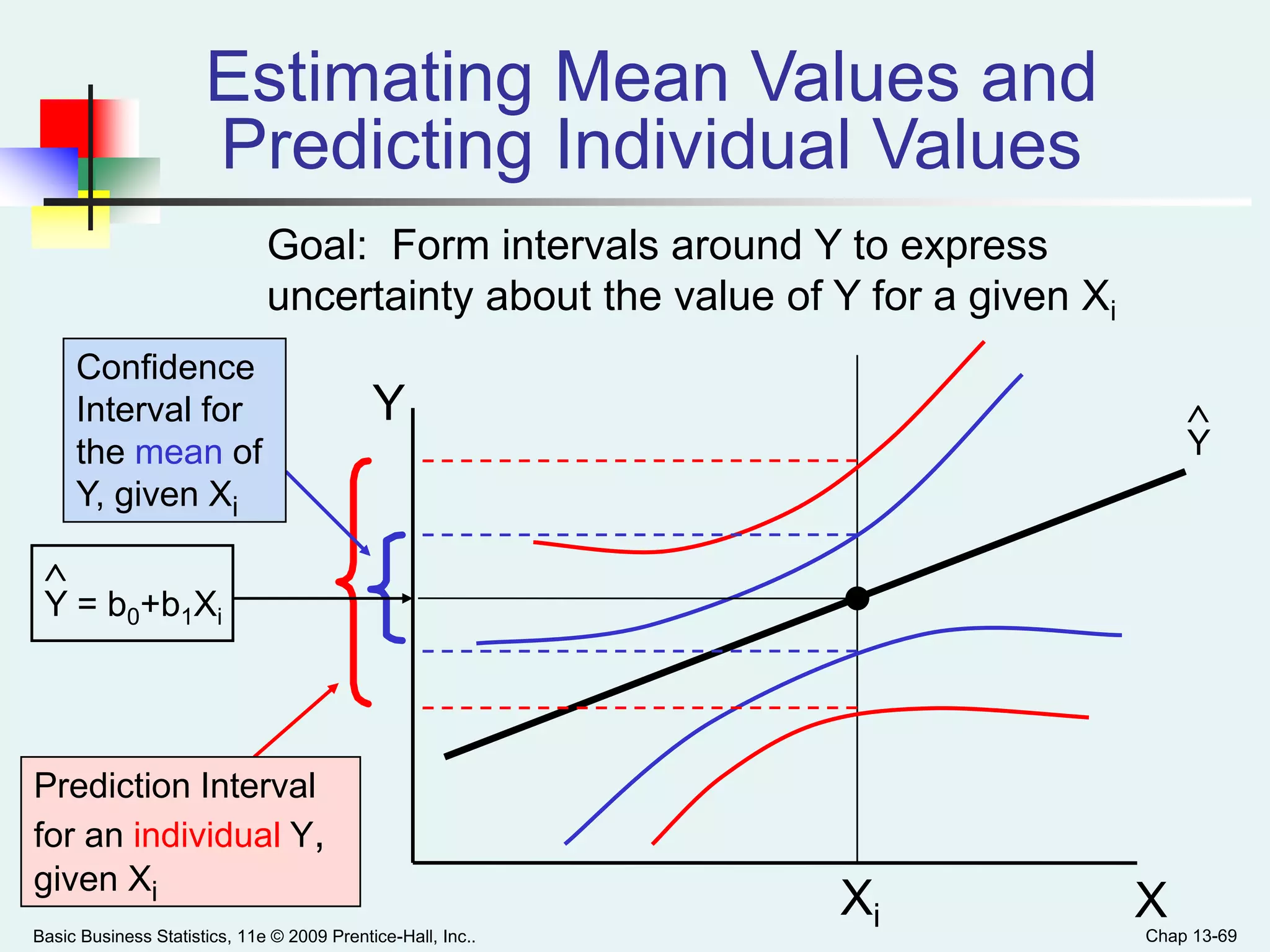
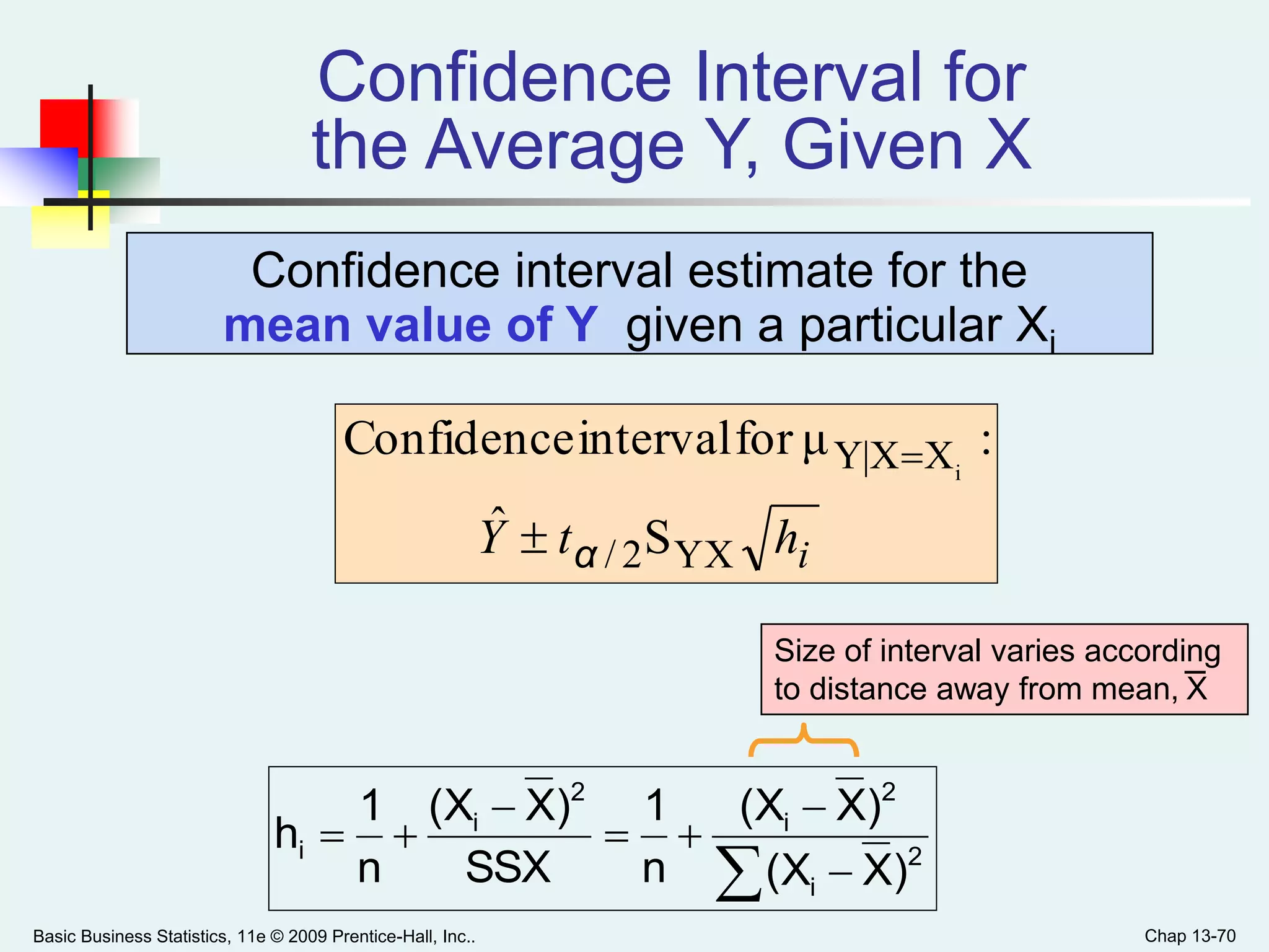
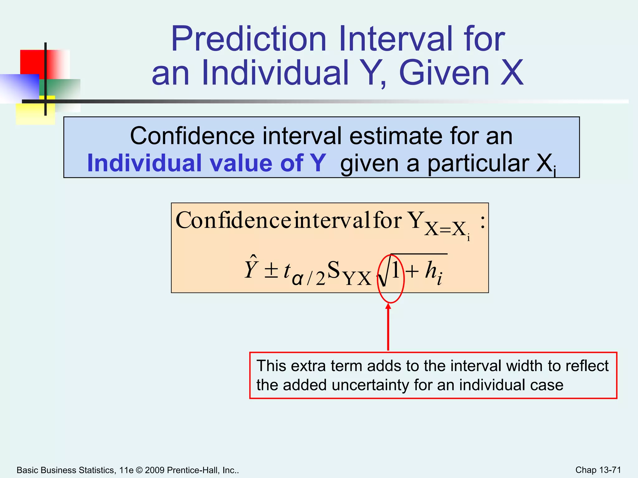
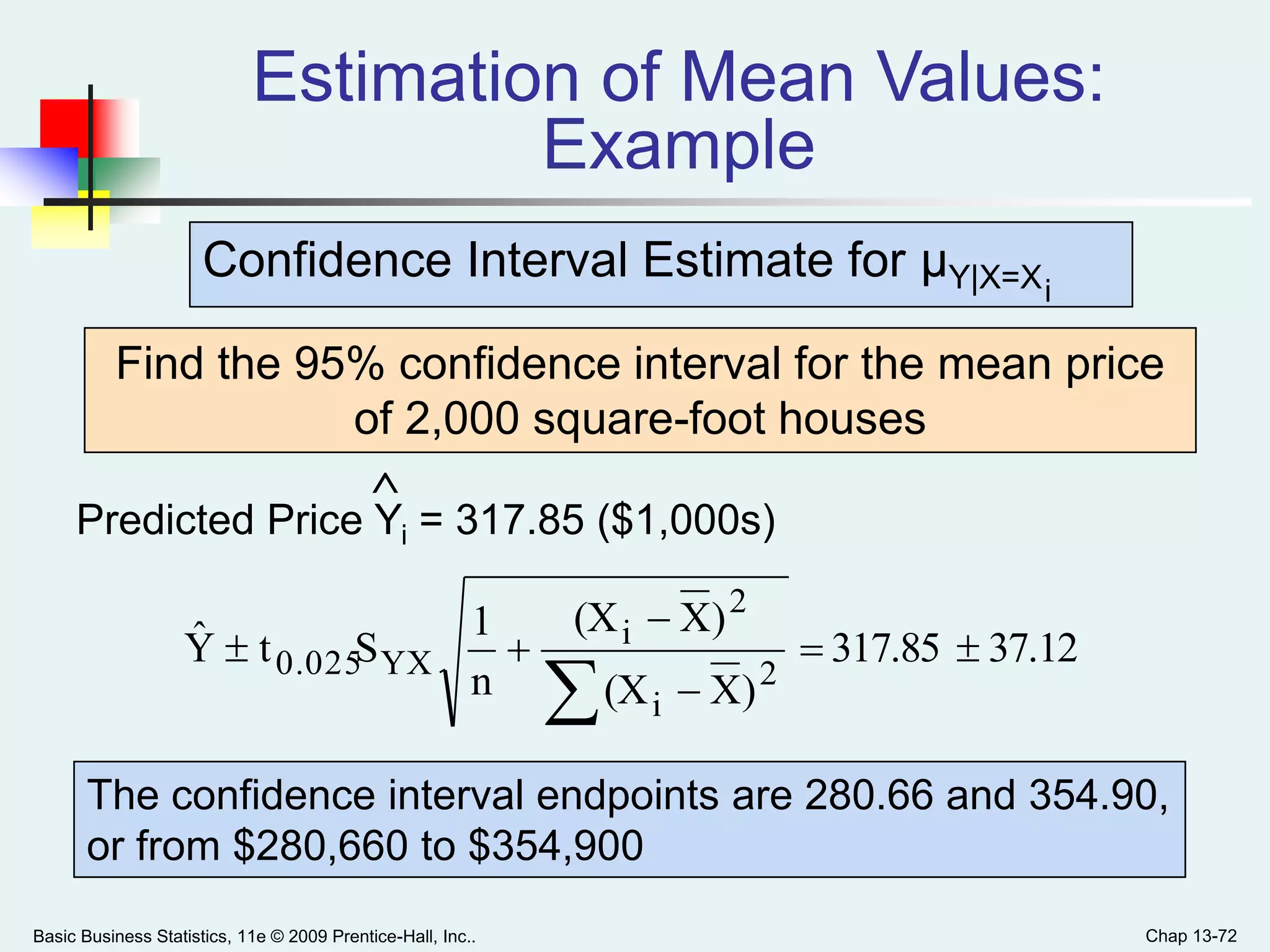
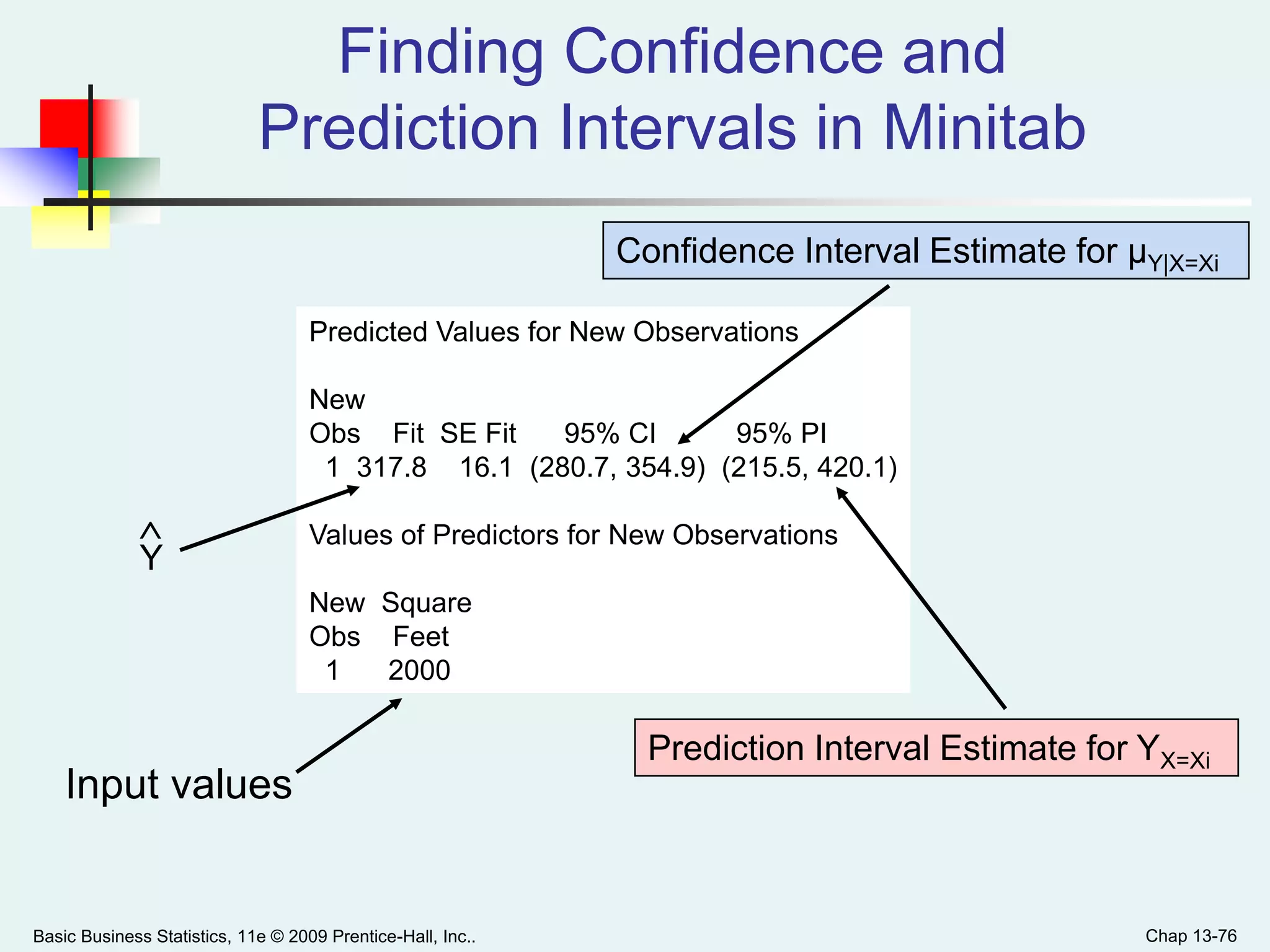
SlideShare a Scribd company logo
1 of 81
Basic Business Statistics, 11e © 2009 Prentice-Hall, Inc. Chap 13-1
Chapter 13
Simple Linear Regression
Basic Business Statistics
11th Edition
Basic Business Statistics, 11e © 2009 Prentice-Hall, Inc.. Chap 13-2
Learning Objectives
In this chapter, you learn:
 How to use regression analysis to predict the value of
a dependent variable based on an independent
variable
 The meaning of the regression coefficients b0 and b1
 How to evaluate the assumptions of regression
analysis and know what to do if the assumptions are
violated
 To make inferences about the slope and correlation
coefficient
 To estimate mean values and predict individual values
Basic Business Statistics, 11e © 2009 Prentice-Hall, Inc.. Chap 13-3
Correlation vs. Regression
 A scatter plot can be used to show the
relationship between two variables
 Correlation analysis is used to measure the
strength of the association (linear relationship)
between two variables
 Correlation is only concerned with strength of the
relationship
 No causal effect is implied with correlation
 Scatter plots were first presented in Ch. 2
 Correlation was first presented in Ch. 3
Basic Business Statistics, 11e © 2009 Prentice-Hall, Inc.. Chap 13-4
Introduction to
Regression Analysis
 Regression analysis is used to:
 Predict the value of a dependent variable based on
the value of at least one independent variable
 Explain the impact of changes in an independent
variable on the dependent variable
Dependent variable: the variable we wish to
predict or explain
Independent variable: the variable used to predict
or explain the dependent
variable
Basic Business Statistics, 11e © 2009 Prentice-Hall, Inc.. Chap 13-5
Simple Linear Regression
Model
 Only one independent variable, X
 Relationship between X and Y is
described by a linear function
 Changes in Y are assumed to be related
to changes in X
Basic Business Statistics, 11e © 2009 Prentice-Hall, Inc.. Chap 13-6
Types of Relationships
Y
X
Y
X
Y
Y
X
X
Linear relationships Curvilinear relationships
Basic Business Statistics, 11e © 2009 Prentice-Hall, Inc.. Chap 13-7
Types of Relationships
Y
X
Y
X
Y
Y
X
X
Strong relationships Weak relationships
(continued)
Basic Business Statistics, 11e © 2009 Prentice-Hall, Inc.. Chap 13-8
Types of Relationships
Y
X
Y
X
No relationship
(continued)
Basic Business Statistics, 11e © 2009 Prentice-Hall, Inc.. Chap 13-9
ii10i εXββY 
Linear component
Simple Linear Regression
Model
Population
Y intercept
Population
Slope
Coefficient
Random
Error
term
Dependent
Variable
Independent
Variable
Random Error
component
Basic Business Statistics, 11e © 2009 Prentice-Hall, Inc.. Chap 13-10
(continued)
Random Error
for this Xi value
Y
X
Observed Value
of Y for Xi
Predicted Value
of Y for Xi
ii10i εXββY 
Xi
Slope = β1
Intercept = β0
εi
Simple Linear Regression
Model
Basic Business Statistics, 11e © 2009 Prentice-Hall, Inc.. Chap 13-11
i10i XbbYˆ 
The simple linear regression equation provides an
estimate of the population regression line
Simple Linear Regression
Equation (Prediction Line)
Estimate of
the regression
intercept
Estimate of the
regression slope
Estimated
(or predicted)
Y value for
observation i
Value of X for
observation i
Basic Business Statistics, 11e © 2009 Prentice-Hall, Inc.. Chap 13-12
The Least Squares Method
b0 and b1 are obtained by finding the values of
that minimize the sum of the squared
differences between Y and :
2
i10i
2
ii ))Xb(b(Ymin)Yˆ(Ymin  
Yˆ
Basic Business Statistics, 11e © 2009 Prentice-Hall, Inc.. Chap 13-13
Finding the Least Squares
Equation
 The coefficients b0 and b1 , and other
regression results in this chapter, will be
found using Excel or Minitab
Formulas are shown in the text for those
who are interested
Basic Business Statistics, 11e © 2009 Prentice-Hall, Inc.. Chap 13-14
 b0 is the estimated average value of Y
when the value of X is zero
 b1 is the estimated change in the
average value of Y as a result of a
one-unit change in X
Interpretation of the
Slope and the Intercept
Basic Business Statistics, 11e © 2009 Prentice-Hall, Inc.. Chap 13-15
Simple Linear Regression
Example
 A real estate agent wishes to examine the
relationship between the selling price of a home
and its size (measured in square feet)
 A random sample of 10 houses is selected
 Dependent variable (Y) = house price in $1000s
 Independent variable (X) = square feet
Basic Business Statistics, 11e © 2009 Prentice-Hall, Inc.. Chap 13-16
Simple Linear Regression
Example: Data
House Price in $1000s
(Y)
Square Feet
(X)
245 1400
312 1600
279 1700
308 1875
199 1100
219 1550
405 2350
324 2450
319 1425
255 1700
Basic Business Statistics, 11e © 2009 Prentice-Hall, Inc.. Chap 13-17
0
50
100
150
200
250
300
350
400
450
0 500 1000 1500 2000 2500 3000
Square Feet
HousePrice($1000s)
Simple Linear Regression
Example: Scatter Plot
House price model: Scatter Plot
Basic Business Statistics, 11e © 2009 Prentice-Hall, Inc.. Chap 13-18
Simple Linear Regression
Example: Using Excel
Basic Business Statistics, 11e © 2009 Prentice-Hall, Inc.. Chap 13-19
Simple Linear Regression
Example: Excel Output
Regression Statistics
Multiple R 0.76211
R Square 0.58082
Adjusted R Square 0.52842
Standard Error 41.33032
Observations 10
ANOVA
df SS MS F Significance F
Regression 1 18934.9348 18934.9348 11.0848 0.01039
Residual 8 13665.5652 1708.1957
Total 9 32600.5000
Coefficients Standard Error t Stat P-value Lower 95% Upper 95%
Intercept 98.24833 58.03348 1.69296 0.12892 -35.57720 232.07386
Square Feet 0.10977 0.03297 3.32938 0.01039 0.03374 0.18580
The regression equation is:
feet)(square0.1097798.24833pricehouse 
Basic Business Statistics, 11e © 2009 Prentice-Hall, Inc.. Chap 13-20
Simple Linear Regression
Example: Minitab Output
The regression equation is
Price = 98.2 + 0.110 Square Feet
Predictor Coef SE Coef T P
Constant 98.25 58.03 1.69 0.129
Square Feet 0.10977 0.03297 3.33 0.010
S = 41.3303 R-Sq = 58.1% R-Sq(adj) = 52.8%
Analysis of Variance
Source DF SS MS F P
Regression 1 18935 18935 11.08 0.010
Residual Error 8 13666 1708
Total 9 32600
The regression
equation is:
house price = 98.24833 +
0.10977 (square feet)
Basic Business Statistics, 11e © 2009 Prentice-Hall, Inc.. Chap 13-21
0
50
100
150
200
250
300
350
400
450
0 500 1000 1500 2000 2500 3000
Square Feet
HousePrice($1000s)
Simple Linear Regression Example:
Graphical Representation
House price model: Scatter Plot and Prediction Line
feet)(square0.1097798.24833pricehouse 
Slope
= 0.10977
Intercept
= 98.248
Basic Business Statistics, 11e © 2009 Prentice-Hall, Inc.. Chap 13-22
Simple Linear Regression
Example: Interpretation of bo
 b0 is the estimated average value of Y when the
value of X is zero (if X = 0 is in the range of
observed X values)
 Because a house cannot have a square footage
of 0, b0 has no practical application
feet)(square0.1097798.24833pricehouse 
Basic Business Statistics, 11e © 2009 Prentice-Hall, Inc.. Chap 13-23
Simple Linear Regression
Example: Interpreting b1
 b1 estimates the change in the average
value of Y as a result of a one-unit
increase in X
 Here, b1 = 0.10977 tells us that the mean value of a
house increases by .10977($1000) = $109.77, on
average, for each additional one square foot of size
feet)(square0.1097798.24833pricehouse 
Basic Business Statistics, 11e © 2009 Prentice-Hall, Inc.. Chap 13-24
317.85
0)0.1098(20098.25
(sq.ft.)0.109898.25pricehouse



Predict the price for a house
with 2000 square feet:
The predicted price for a house with 2000
square feet is 317.85($1,000s) = $317,850
Simple Linear Regression
Example: Making Predictions
Basic Business Statistics, 11e © 2009 Prentice-Hall, Inc.. Chap 13-25
0
50
100
150
200
250
300
350
400
450
0 500 1000 1500 2000 2500 3000
Square Feet
HousePrice($1000s)
Simple Linear Regression
Example: Making Predictions
 When using a regression model for prediction,
only predict within the relevant range of data
Relevant range for
interpolation
Do not try to
extrapolate
beyond the range
of observed X’s
Basic Business Statistics, 11e © 2009 Prentice-Hall, Inc.. Chap 13-26
Measures of Variation
 Total variation is made up of two parts:
SSESSRSST 
Total Sum of
Squares
Regression Sum
of Squares
Error Sum of
Squares
  2
i )YY(SST   2
ii )YˆY(SSE  2
i )YYˆ(SSR
where:
= Mean value of the dependent variable
Yi = Observed value of the dependent variable
= Predicted value of Y for the given Xi valueiYˆ
Y
Basic Business Statistics, 11e © 2009 Prentice-Hall, Inc.. Chap 13-27
 SST = total sum of squares (Total Variation)
 Measures the variation of the Yi values around their
mean Y
 SSR = regression sum of squares (Explained Variation)
 Variation attributable to the relationship between X
and Y
 SSE = error sum of squares (Unexplained Variation)
 Variation in Y attributable to factors other than X
(continued)
Measures of Variation
Basic Business Statistics, 11e © 2009 Prentice-Hall, Inc.. Chap 13-28
(continued)
Xi
Y
X
Yi
SST = (Yi - Y)2
SSE = (Yi - Yi )2

SSR = (Yi - Y)2

_
_
_
Y

Y
Y
_
Y

Measures of Variation
Basic Business Statistics, 11e © 2009 Prentice-Hall, Inc.. Chap 13-29
 The coefficient of determination is the portion
of the total variation in the dependent variable
that is explained by variation in the
independent variable
 The coefficient of determination is also called
r-squared and is denoted as r2
Coefficient of Determination, r2
1r0 2
note:
squaresofsum
squaresofregression2
total
sum
SST
SSR
r 
Basic Business Statistics, 11e © 2009 Prentice-Hall, Inc.. Chap 13-30
r2 = 1
Examples of Approximate
r2 Values
Y
X
Y
X
r2 = 1
r2 = 1
Perfect linear relationship
between X and Y:
100% of the variation in Y is
explained by variation in X
Basic Business Statistics, 11e © 2009 Prentice-Hall, Inc.. Chap 13-31
Examples of Approximate
r2 Values
Y
X
Y
X
0 < r2 < 1
Weaker linear relationships
between X and Y:
Some but not all of the
variation in Y is explained
by variation in X
Basic Business Statistics, 11e © 2009 Prentice-Hall, Inc.. Chap 13-32
Examples of Approximate
r2 Values
r2 = 0
No linear relationship
between X and Y:
The value of Y does not
depend on X. (None of the
variation in Y is explained
by variation in X)
Y
X
r2 = 0
Basic Business Statistics, 11e © 2009 Prentice-Hall, Inc.. Chap 13-33
Simple Linear Regression Example:
Coefficient of Determination, r2 in Excel
Regression Statistics
Multiple R 0.76211
R Square 0.58082
Adjusted R Square 0.52842
Standard Error 41.33032
Observations 10
ANOVA
df SS MS F Significance F
Regression 1 18934.9348 18934.9348 11.0848 0.01039
Residual 8 13665.5652 1708.1957
Total 9 32600.5000
Coefficients Standard Error t Stat P-value Lower 95% Upper 95%
Intercept 98.24833 58.03348 1.69296 0.12892 -35.57720 232.07386
Square Feet 0.10977 0.03297 3.32938 0.01039 0.03374 0.18580
58.08% of the variation in
house prices is explained by
variation in square feet
0.58082
32600.5000
18934.9348
SST
SSR
r2

Basic Business Statistics, 11e © 2009 Prentice-Hall, Inc.. Chap 13-34
Simple Linear Regression Example:
Coefficient of Determination, r2 in Minitab
The regression equation is
Price = 98.2 + 0.110 Square Feet
Predictor Coef SE Coef T P
Constant 98.25 58.03 1.69 0.129
Square Feet 0.10977 0.03297 3.33 0.010
S = 41.3303 R-Sq = 58.1% R-Sq(adj) = 52.8%
Analysis of Variance
Source DF SS MS F P
Regression 1 18935 18935 11.08 0.010
Residual Error 8 13666 1708
Total 9 32600
0.58082
32600.5000
18934.9348
SST
SSR
r2

58.08% of the variation in
house prices is explained
by variation in square feet
Basic Business Statistics, 11e © 2009 Prentice-Hall, Inc.. Chap 13-35
Standard Error of Estimate
 The standard deviation of the variation of
observations around the regression line is
estimated by
2
)ˆ(
2
1
2







n
YY
n
SSE
S
n
i
ii
YX
Where
SSE = error sum of squares
n = sample size
Basic Business Statistics, 11e © 2009 Prentice-Hall, Inc.. Chap 13-36
Simple Linear Regression Example:
Standard Error of Estimate in Excel
Regression Statistics
Multiple R 0.76211
R Square 0.58082
Adjusted R Square 0.52842
Standard Error 41.33032
Observations 10
ANOVA
df SS MS F Significance F
Regression 1 18934.9348 18934.9348 11.0848 0.01039
Residual 8 13665.5652 1708.1957
Total 9 32600.5000
Coefficients Standard Error t Stat P-value Lower 95% Upper 95%
Intercept 98.24833 58.03348 1.69296 0.12892 -35.57720 232.07386
Square Feet 0.10977 0.03297 3.32938 0.01039 0.03374 0.18580
41.33032SYX 
Basic Business Statistics, 11e © 2009 Prentice-Hall, Inc.. Chap 13-37
Simple Linear Regression Example:
Standard Error of Estimate in Minitab
The regression equation is
Price = 98.2 + 0.110 Square Feet
Predictor Coef SE Coef T P
Constant 98.25 58.03 1.69 0.129
Square Feet 0.10977 0.03297 3.33 0.010
S = 41.3303 R-Sq = 58.1% R-Sq(adj) = 52.8%
Analysis of Variance
Source DF SS MS F P
Regression 1 18935 18935 11.08 0.010
Residual Error 8 13666 1708
Total 9 32600
41.33032SYX 
Basic Business Statistics, 11e © 2009 Prentice-Hall, Inc.. Chap 13-38
Comparing Standard Errors
YY
X X
YX
Ssmall
YX
Slarge
SYX is a measure of the variation of observed
Y values from the regression line
The magnitude of SYX should always be judged relative to the
size of the Y values in the sample data
i.e., SYX = $41.33K is moderately small relative to house prices in
the $200K - $400K range
Basic Business Statistics, 11e © 2009 Prentice-Hall, Inc.. Chap 13-39
Assumptions of Regression
L.I.N.E
 Linearity
 The relationship between X and Y is linear
 Independence of Errors
 Error values are statistically independent
 Normality of Error
 Error values are normally distributed for any given
value of X
 Equal Variance (also called homoscedasticity)
 The probability distribution of the errors has constant
variance
Basic Business Statistics, 11e © 2009 Prentice-Hall, Inc.. Chap 13-40
Residual Analysis
 The residual for observation i, ei, is the difference
between its observed and predicted value
 Check the assumptions of regression by examining the
residuals
 Examine for linearity assumption
 Evaluate independence assumption
 Evaluate normal distribution assumption
 Examine for constant variance for all levels of X
(homoscedasticity)
 Graphical Analysis of Residuals
 Can plot residuals vs. X
iii YˆYe 
Basic Business Statistics, 11e © 2009 Prentice-Hall, Inc.. Chap 13-41
Residual Analysis for Linearity
Not Linear Linear

x
residuals
x
Y
x
Y
x
residuals
Basic Business Statistics, 11e © 2009 Prentice-Hall, Inc.. Chap 13-42
Residual Analysis for
Independence
Not Independent
Independent
X
X
residuals
residuals
X
residuals

Basic Business Statistics, 11e © 2009 Prentice-Hall, Inc.. Chap 13-43
Checking for Normality
 Examine the Stem-and-Leaf Display of the
Residuals
 Examine the Boxplot of the Residuals
 Examine the Histogram of the Residuals
 Construct a Normal Probability Plot of the
Residuals
Basic Business Statistics, 11e © 2009 Prentice-Hall, Inc.. Chap 13-44
Residual Analysis for Normality
Percent
Residual
When using a normal probability plot, normal
errors will approximately display in a straight line
-3 -2 -1 0 1 2 3
0
100
Basic Business Statistics, 11e © 2009 Prentice-Hall, Inc.. Chap 13-45
Residual Analysis for
Equal Variance
Non-constant variance  Constant variance
x x
Y
x x
Y
residuals
residuals
Basic Business Statistics, 11e © 2009 Prentice-Hall, Inc.. Chap 13-46
House Price Model Residual Plot
-60
-40
-20
0
20
40
60
80
0 1000 2000 3000
Square Feet
Residuals
Simple Linear Regression
Example: Excel Residual Output
RESIDUAL OUTPUT
Predicted
House Price Residuals
1 251.92316 -6.923162
2 273.87671 38.12329
3 284.85348 -5.853484
4 304.06284 3.937162
5 218.99284 -19.99284
6 268.38832 -49.38832
7 356.20251 48.79749
8 367.17929 -43.17929
9 254.6674 64.33264
10 284.85348 -29.85348
Does not appear to violate
any regression assumptions
Basic Business Statistics, 11e © 2009 Prentice-Hall, Inc.. Chap 13-47
 Used when data are collected over time to
detect if autocorrelation is present
 Autocorrelation exists if residuals in one
time period are related to residuals in
another period
Measuring Autocorrelation:
The Durbin-Watson Statistic
Basic Business Statistics, 11e © 2009 Prentice-Hall, Inc.. Chap 13-48
Autocorrelation
 Autocorrelation is correlation of the errors
(residuals) over time
 Violates the regression assumption that
residuals are random and independent
Time (t) Residual Plot
-15
-10
-5
0
5
10
15
0 2 4 6 8
Time (t)
Residuals
 Here, residuals show a
cyclic pattern, not
random. Cyclical
patterns are a sign of
positive autocorrelation
Basic Business Statistics, 11e © 2009 Prentice-Hall, Inc.. Chap 13-49
The Durbin-Watson Statistic





 n
1i
2
i
n
2i
2
1ii
e
)ee(
D
 The possible range is 0 ≤ D ≤ 4
 D should be close to 2 if H0 is true
 D less than 2 may signal positive
autocorrelation, D greater than 2 may
signal negative autocorrelation
 The Durbin-Watson statistic is used to test for
autocorrelation
H0: residuals are not correlated
H1: positive autocorrelation is present
Basic Business Statistics, 11e © 2009 Prentice-Hall, Inc.. Chap 13-50
Testing for Positive
Autocorrelation
 Calculate the Durbin-Watson test statistic = D
(The Durbin-Watson Statistic can be found using Excel or Minitab)
Decision rule: reject H0 if D < dL
H0: positive autocorrelation does not exist
H1: positive autocorrelation is present
0 dU 2dL
Reject H0 Do not reject H0
 Find the values dL and dU from the Durbin-Watson table
(for sample size n and number of independent variables k)
Inconclusive
Basic Business Statistics, 11e © 2009 Prentice-Hall, Inc.. Chap 13-51
 Suppose we have the following time series
data:
 Is there autocorrelation?
y = 30.65 + 4.7038x
R
2
= 0.8976
0
20
40
60
80
100
120
140
160
0 5 10 15 20 25 30
Time
Sales
Testing for Positive
Autocorrelation
(continued)
Basic Business Statistics, 11e © 2009 Prentice-Hall, Inc.. Chap 13-52
 Example with n = 25:
Durbin-Watson Calculations
Sum of Squared
Difference of Residuals 3296.18
Sum of Squared
Residuals 3279.98
Durbin-Watson
Statistic 1.00494
y = 30.65 + 4.7038x
R
2
= 0.8976
0
20
40
60
80
100
120
140
160
0 5 10 15 20 25 30
Time
Sales
Testing for Positive
Autocorrelation
(continued)
Excel/PHStat output:
1.00494
3279.98
3296.18
e
)e(e
D n
1i
2
i
n
2i
2
1ii








Basic Business Statistics, 11e © 2009 Prentice-Hall, Inc.. Chap 13-53
 Here, n = 25 and there is k = 1 one independent variable
 Using the Durbin-Watson table, dL = 1.29 and dU = 1.45
 D = 1.00494 < dL = 1.29, so reject H0 and conclude that
significant positive autocorrelation exists
Testing for Positive
Autocorrelation
(continued)
Decision: reject H0 since
D = 1.00494 < dL
0 dU=1.45 2dL=1.29
Reject H0 Do not reject H0Inconclusive
Basic Business Statistics, 11e © 2009 Prentice-Hall, Inc.. Chap 13-54
Inferences About the Slope
 The standard error of the regression slope
coefficient (b1) is estimated by
 

2
i
YXYX
b
)X(X
S
SSX
S
S 1
where:
= Estimate of the standard error of the slope
= Standard error of the estimate
1bS
2n
SSE
SYX


Basic Business Statistics, 11e © 2009 Prentice-Hall, Inc.. Chap 13-55
Inferences About the Slope:
t Test
 t test for a population slope
 Is there a linear relationship between X and Y?
 Null and alternative hypotheses
 H0: β1 = 0 (no linear relationship)
 H1: β1 ≠ 0 (linear relationship does exist)
 Test statistic
1
b
11
STAT
S
βb
t


2nd.f. 
where:
b1 = regression slope
coefficient
β1 = hypothesized slope
Sb1 = standard
error of the slope
Basic Business Statistics, 11e © 2009 Prentice-Hall, Inc.. Chap 13-56
Inferences About the Slope:
t Test Example
House Price
in $1000s
(y)
Square Feet
(x)
245 1400
312 1600
279 1700
308 1875
199 1100
219 1550
405 2350
324 2450
319 1425
255 1700
(sq.ft.)0.109898.25pricehouse 
Estimated Regression Equation:
The slope of this model is 0.1098
Is there a relationship between the
square footage of the house and its
sales price?
Basic Business Statistics, 11e © 2009 Prentice-Hall, Inc.. Chap 13-57
Inferences About the Slope:
t Test Example
H0: β1 = 0
H1: β1 ≠ 0From Excel output:
Coefficients Standard Error t Stat P-value
Intercept 98.24833 58.03348 1.69296 0.12892
Square Feet 0.10977 0.03297 3.32938 0.01039
1bSb1
329383
032970
0109770
S
βb
t
1
b
11
STAT
.
.
.





Predictor Coef SE Coef T P
Constant 98.25 58.03 1.69 0.129
Square Feet 0.10977 0.03297 3.33 0.010
From Minitab output:
b1 1bS
Basic Business Statistics, 11e © 2009 Prentice-Hall, Inc.. Chap 13-58
Inferences About the Slope:
t Test Example
Test Statistic: tSTAT = 3.329
There is sufficient evidence
that square footage affects
house price
Decision: Reject H0
Reject H0Reject H0
a/2=.025
-tα/2
Do not reject H0
0
tα/2
a/2=.025
-2.3060 2.3060 3.329
d.f. = 10- 2 = 8
H0: β1 = 0
H1: β1 ≠ 0
Basic Business Statistics, 11e © 2009 Prentice-Hall, Inc.. Chap 13-59
Inferences About the Slope:
t Test ExampleH0: β1 = 0
H1: β1 ≠ 0
From Excel output:
Coefficients Standard Error t Stat P-value
Intercept 98.24833 58.03348 1.69296 0.12892
Square Feet 0.10977 0.03297 3.32938 0.01039
p-value
There is sufficient evidence that
square footage affects house price.
Decision: Reject H0, since p-value < α
Predictor Coef SE Coef T P
Constant 98.25 58.03 1.69 0.129
Square Feet 0.10977 0.03297 3.33 0.010
From Minitab output:
Basic Business Statistics, 11e © 2009 Prentice-Hall, Inc.. Chap 13-60
F Test for Significance
 F Test statistic:
where
MSE
MSR
FSTAT 
1kn
SSE
MSE
k
SSR
MSR



where FSTAT follows an F distribution with k numerator and (n – k - 1)
denominator degrees of freedom
(k = the number of independent variables in the regression model)
Basic Business Statistics, 11e © 2009 Prentice-Hall, Inc.. Chap 13-61
F-Test for Significance
Excel Output
Regression Statistics
Multiple R 0.76211
R Square 0.58082
Adjusted R Square 0.52842
Standard Error 41.33032
Observations 10
ANOVA
df SS MS F Significance F
Regression 1 18934.9348 18934.9348 11.0848 0.01039
Residual 8 13665.5652 1708.1957
Total 9 32600.5000
11.0848
1708.1957
18934.9348
MSE
MSR
FSTAT 
With 1 and 8 degrees
of freedom
p-value for
the F-Test
Basic Business Statistics, 11e © 2009 Prentice-Hall, Inc.. Chap 13-62
F-Test for Significance
Minitab Output
Analysis of Variance
Source DF SS MS F P
Regression 1 18935 18935 11.08 0.010
Residual Error 8 13666 1708
Total 9 32600
11.0848
1708.1957
18934.9348
MSE
MSR
FSTAT With 1 and 8 degrees
of freedom
p-value for
the F-Test
Basic Business Statistics, 11e © 2009 Prentice-Hall, Inc.. Chap 13-63
H0: β1 = 0
H1: β1 ≠ 0
a = .05
df1= 1 df2 = 8
Test Statistic:
Decision:
Conclusion:
Reject H0 at a = 0.05
There is sufficient evidence that
house size affects selling price0
a = .05
F.05 = 5.32
Reject H0Do not
reject H0
11.08FSTAT 
MSE
MSR
Critical
Value:
Fa = 5.32
F Test for Significance
(continued)
F
Basic Business Statistics, 11e © 2009 Prentice-Hall, Inc.. Chap 13-64
Confidence Interval Estimate
for the Slope
Confidence Interval Estimate of the Slope:
Excel Printout for House Prices:
At 95% level of confidence, the confidence interval for
the slope is (0.0337, 0.1858)
1
b2/1 Sb αt
Coefficients Standard Error t Stat P-value Lower 95% Upper 95%
Intercept 98.24833 58.03348 1.69296 0.12892 -35.57720 232.07386
Square Feet 0.10977 0.03297 3.32938 0.01039 0.03374 0.18580
d.f. = n - 2
Basic Business Statistics, 11e © 2009 Prentice-Hall, Inc.. Chap 13-65
Since the units of the house price variable is
$1000s, we are 95% confident that the average
impact on sales price is between $33.74 and
$185.80 per square foot of house size
Coefficients Standard Error t Stat P-value Lower 95% Upper 95%
Intercept 98.24833 58.03348 1.69296 0.12892 -35.57720 232.07386
Square Feet 0.10977 0.03297 3.32938 0.01039 0.03374 0.18580
This 95% confidence interval does not include 0.
Conclusion: There is a significant relationship between
house price and square feet at the .05 level of significance
Confidence Interval Estimate
for the Slope
(continued)
Basic Business Statistics, 11e © 2009 Prentice-Hall, Inc.. Chap 13-66
t Test for a Correlation Coefficient
 Hypotheses
H0: ρ = 0 (no correlation between X and Y)
H1: ρ ≠ 0 (correlation exists)
 Test statistic
(with n – 2 degrees of freedom)
2n
r1
ρ-r
t
2
STAT



0bifrr
0bifrr
where
1
2
1
2


Basic Business Statistics, 11e © 2009 Prentice-Hall, Inc.. Chap 13-67
t-test For A Correlation Coefficient
Is there evidence of a linear relationship
between square feet and house price at the
.05 level of significance?
H0: ρ = 0 (No correlation)
H1: ρ ≠ 0 (correlation exists)
a =.05 , df = 10 - 2 = 8
3.329
210
.7621
0.762
2n
r1
ρr
t
22
STAT 








(continued)
Basic Business Statistics, 11e © 2009 Prentice-Hall, Inc.. Chap 13-68
t-test For A Correlation Coefficient
Conclusion:
There is
evidence of a
linear association
at the 5% level of
significance
Decision:
Reject H0
Reject H0Reject H0
a/2=.025
-tα/2
Do not reject H0
0
tα/2
a/2=.025
-2.3060 2.3060
3.329
d.f. = 10-2 = 8
3.329
210
.7621
0.762
2n
r1
ρr
t
22
STAT 








(continued)
Basic Business Statistics, 11e © 2009 Prentice-Hall, Inc.. Chap 13-69
Estimating Mean Values and
Predicting Individual Values
Y
XXi
Y = b0+b1Xi

Confidence
Interval for
the mean of
Y, given Xi
Prediction Interval
for an individual Y,
given Xi
Goal: Form intervals around Y to express
uncertainty about the value of Y for a given Xi
Y

Basic Business Statistics, 11e © 2009 Prentice-Hall, Inc.. Chap 13-70
Confidence Interval for
the Average Y, Given X
Confidence interval estimate for the
mean value of Y given a particular Xi
Size of interval varies according
to distance away from mean, X
ihtY YX2/
XX|Y
Sˆ
:μforintervalConfidence
i
α

 



 2
i
2
i
2
i
i
)X(X
)X(X
n
1
SSX
)X(X
n
1
h
Basic Business Statistics, 11e © 2009 Prentice-Hall, Inc.. Chap 13-71
Prediction Interval for
an Individual Y, Given X
Confidence interval estimate for an
Individual value of Y given a particular Xi
This extra term adds to the interval width to reflect
the added uncertainty for an individual case
ihtY 

1Sˆ
:YforintervalConfidence
YX2/
XX i
α
Basic Business Statistics, 11e © 2009 Prentice-Hall, Inc.. Chap 13-72
Estimation of Mean Values:
Example
Find the 95% confidence interval for the mean price
of 2,000 square-foot houses
Predicted Price Yi = 317.85 ($1,000s)

Confidence Interval Estimate for μY|X=X
37.12317.85
)X(X
)X(X
n
1
StYˆ
2
i
2
i
YX0.025 




The confidence interval endpoints are 280.66 and 354.90,
or from $280,660 to $354,900
i
Basic Business Statistics, 11e © 2009 Prentice-Hall, Inc.. Chap 13-73
Estimation of Individual Values:
Example
Find the 95% prediction interval for an individual
house with 2,000 square feet
Predicted Price Yi = 317.85 ($1,000s)

Prediction Interval Estimate for YX=X
102.28317.85
)X(X
)X(X
n
1
1StYˆ
2
i
2
i
YX0.025 




The prediction interval endpoints are 215.50 and 420.07,
or from $215,500 to $420,070
i
Basic Business Statistics, 11e © 2009 Prentice-Hall, Inc.. Chap 13-74
Finding Confidence and
Prediction Intervals in Excel
 From Excel, use
PHStat | regression | simple linear regression …
 Check the
“confidence and prediction interval for X=”
box and enter the X-value and confidence level
desired
Basic Business Statistics, 11e © 2009 Prentice-Hall, Inc.. Chap 13-75
Input values
Finding Confidence and
Prediction Intervals in Excel
(continued)
Confidence Interval Estimate for μY|X=Xi
Prediction Interval Estimate for YX=Xi
Y

Basic Business Statistics, 11e © 2009 Prentice-Hall, Inc.. Chap 13-76
Finding Confidence and
Prediction Intervals in Minitab
Predicted Values for New Observations
New
Obs Fit SE Fit 95% CI 95% PI
1 317.8 16.1 (280.7, 354.9) (215.5, 420.1)
Values of Predictors for New Observations
New Square
Obs Feet
1 2000
Y

Input values
Confidence Interval Estimate for μY|X=Xi
Prediction Interval Estimate for YX=Xi
Basic Business Statistics, 11e © 2009 Prentice-Hall, Inc.. Chap 13-77
Pitfalls of Regression Analysis
 Lacking an awareness of the assumptions
underlying least-squares regression
 Not knowing how to evaluate the assumptions
 Not knowing the alternatives to least-squares
regression if a particular assumption is violated
 Using a regression model without knowledge of
the subject matter
 Extrapolating outside the relevant range
Basic Business Statistics, 11e © 2009 Prentice-Hall, Inc.. Chap 13-78
Strategies for Avoiding
the Pitfalls of Regression
 Start with a scatter plot of X vs. Y to observe
possible relationship
 Perform residual analysis to check the
assumptions
 Plot the residuals vs. X to check for violations of
assumptions such as homoscedasticity
 Use a histogram, stem-and-leaf display, boxplot,
or normal probability plot of the residuals to
uncover possible non-normality
Basic Business Statistics, 11e © 2009 Prentice-Hall, Inc.. Chap 13-79
Strategies for Avoiding
the Pitfalls of Regression
 If there is violation of any assumption, use
alternative methods or models
 If there is no evidence of assumption violation,
then test for the significance of the regression
coefficients and construct confidence intervals
and prediction intervals
 Avoid making predictions or forecasts outside
the relevant range
(continued)
Basic Business Statistics, 11e © 2009 Prentice-Hall, Inc.. Chap 13-80
Chapter Summary
 Introduced types of regression models
 Reviewed assumptions of regression and
correlation
 Discussed determining the simple linear
regression equation
 Described measures of variation
 Discussed residual analysis
 Addressed measuring autocorrelation
Basic Business Statistics, 11e © 2009 Prentice-Hall, Inc.. Chap 13-81
Chapter Summary
 Described inference about the slope
 Discussed correlation -- measuring the strength
of the association
 Addressed estimation of mean values and
prediction of individual values
 Discussed possible pitfalls in regression and
recommended strategies to avoid them
(continued)

More Related Content

What's hot

The Normal Distribution and Other Continuous Distributions
The Normal Distribution and Other Continuous DistributionsThe Normal Distribution and Other Continuous Distributions
The Normal Distribution and Other Continuous DistributionsYesica Adicondro
 
Bbs11 ppt ch10
Bbs11 ppt ch10Bbs11 ppt ch10
Bbs11 ppt ch10Tuul Tuul
 
Bbs11 ppt ch05
Bbs11 ppt ch05Bbs11 ppt ch05
Bbs11 ppt ch05Tuul Tuul
 
Confidence Interval Estimation
Confidence Interval EstimationConfidence Interval Estimation
Confidence Interval EstimationYesica Adicondro
 
Applied Business Statistics ,ken black , ch 2
Applied Business Statistics ,ken black , ch 2Applied Business Statistics ,ken black , ch 2
Applied Business Statistics ,ken black , ch 2AbdelmonsifFadl
 
Applied Business Statistics ,ken black , ch 5
Applied Business Statistics ,ken black , ch 5Applied Business Statistics ,ken black , ch 5
Applied Business Statistics ,ken black , ch 5AbdelmonsifFadl
 
Applied Business Statistics ,ken black , ch 4
Applied Business Statistics ,ken black , ch 4Applied Business Statistics ,ken black , ch 4
Applied Business Statistics ,ken black , ch 4AbdelmonsifFadl
 
Chap03 numerical descriptive measures
Chap03 numerical descriptive measuresChap03 numerical descriptive measures
Chap03 numerical descriptive measuresUni Azza Aunillah
 
Chapter 6 simple regression and correlation
Chapter 6 simple regression and correlationChapter 6 simple regression and correlation
Chapter 6 simple regression and correlationRione Drevale
 
Chapter 06
Chapter 06Chapter 06
Chapter 06bmcfad01
 
Chap05 discrete probability distributions
Chap05 discrete probability distributionsChap05 discrete probability distributions
Chap05 discrete probability distributionsUni Azza Aunillah
 
Introduction to Statistics
Introduction to StatisticsIntroduction to Statistics
Introduction to StatisticsAnjan Mahanta
 
Probability powerpoint
Probability powerpointProbability powerpoint
Probability powerpointTiffany Deegan
 

What's hot (20)

The Normal Distribution and Other Continuous Distributions
The Normal Distribution and Other Continuous DistributionsThe Normal Distribution and Other Continuous Distributions
The Normal Distribution and Other Continuous Distributions
 
chap07.ppt
chap07.pptchap07.ppt
chap07.ppt
 
Bbs11 ppt ch10
Bbs11 ppt ch10Bbs11 ppt ch10
Bbs11 ppt ch10
 
Bbs11 ppt ch05
Bbs11 ppt ch05Bbs11 ppt ch05
Bbs11 ppt ch05
 
Confidence Interval Estimation
Confidence Interval EstimationConfidence Interval Estimation
Confidence Interval Estimation
 
Simple Linear Regression
Simple Linear RegressionSimple Linear Regression
Simple Linear Regression
 
Applied Business Statistics ,ken black , ch 2
Applied Business Statistics ,ken black , ch 2Applied Business Statistics ,ken black , ch 2
Applied Business Statistics ,ken black , ch 2
 
Applied Business Statistics ,ken black , ch 5
Applied Business Statistics ,ken black , ch 5Applied Business Statistics ,ken black , ch 5
Applied Business Statistics ,ken black , ch 5
 
Applied Business Statistics ,ken black , ch 4
Applied Business Statistics ,ken black , ch 4Applied Business Statistics ,ken black , ch 4
Applied Business Statistics ,ken black , ch 4
 
Chap03 numerical descriptive measures
Chap03 numerical descriptive measuresChap03 numerical descriptive measures
Chap03 numerical descriptive measures
 
Simple Regression
Simple RegressionSimple Regression
Simple Regression
 
Chapter 6 simple regression and correlation
Chapter 6 simple regression and correlationChapter 6 simple regression and correlation
Chapter 6 simple regression and correlation
 
Chapter 06
Chapter 06Chapter 06
Chapter 06
 
An Overview of Simple Linear Regression
An Overview of Simple Linear RegressionAn Overview of Simple Linear Regression
An Overview of Simple Linear Regression
 
Chap05 discrete probability distributions
Chap05 discrete probability distributionsChap05 discrete probability distributions
Chap05 discrete probability distributions
 
Chap07 interval estimation
Chap07 interval estimationChap07 interval estimation
Chap07 interval estimation
 
Introduction to Statistics
Introduction to StatisticsIntroduction to Statistics
Introduction to Statistics
 
Chap12 simple regression
Chap12 simple regressionChap12 simple regression
Chap12 simple regression
 
Chapter 1 what is statistics
Chapter 1 what is statisticsChapter 1 what is statistics
Chapter 1 what is statistics
 
Probability powerpoint
Probability powerpointProbability powerpoint
Probability powerpoint
 

Similar to Bbs11 ppt ch13

Newbold_chap12.ppt
Newbold_chap12.pptNewbold_chap12.ppt
Newbold_chap12.pptcfisicaster
 
simple regression-1.pdf
simple regression-1.pdfsimple regression-1.pdf
simple regression-1.pdfBabulShaikh1
 
Chapter 4 power point presentation Regression models
Chapter 4 power point presentation Regression modelsChapter 4 power point presentation Regression models
Chapter 4 power point presentation Regression modelsJustinXerri
 
linear Regression, multiple Regression and Annova
linear Regression, multiple Regression and Annovalinear Regression, multiple Regression and Annova
linear Regression, multiple Regression and AnnovaMansi Rastogi
 
lecture No. 3a.ppt
lecture No. 3a.pptlecture No. 3a.ppt
lecture No. 3a.pptHamidUllah50
 
20 ms-me-amd-06 (simple linear regression)
20 ms-me-amd-06 (simple linear regression)20 ms-me-amd-06 (simple linear regression)
20 ms-me-amd-06 (simple linear regression)HassanShah124
 
Concept of Regression in Research Methodology.pdf
Concept of Regression in Research Methodology.pdfConcept of Regression in Research Methodology.pdf
Concept of Regression in Research Methodology.pdfBalamurugan M
 
Bbs11 ppt ch17
Bbs11 ppt ch17Bbs11 ppt ch17
Bbs11 ppt ch17Tuul Tuul
 
Simple regression model
Simple regression modelSimple regression model
Simple regression modelMidoTami
 
multiple regression model building
 multiple regression model building multiple regression model building
multiple regression model buildingYesica Adicondro
 
Acem linearregression
Acem linearregressionAcem linearregression
Acem linearregressionAastha Kohli
 

Similar to Bbs11 ppt ch13 (20)

Chap11 simple regression
Chap11 simple regressionChap11 simple regression
Chap11 simple regression
 
Linear regression
Linear regressionLinear regression
Linear regression
 
Newbold_chap12.ppt
Newbold_chap12.pptNewbold_chap12.ppt
Newbold_chap12.ppt
 
simple regression-1.pdf
simple regression-1.pdfsimple regression-1.pdf
simple regression-1.pdf
 
chap12.pptx
chap12.pptxchap12.pptx
chap12.pptx
 
Chapter 4 power point presentation Regression models
Chapter 4 power point presentation Regression modelsChapter 4 power point presentation Regression models
Chapter 4 power point presentation Regression models
 
metod linearne regresije
 metod linearne  regresije metod linearne  regresije
metod linearne regresije
 
2.1 regression
2.1 regression2.1 regression
2.1 regression
 
linear Regression, multiple Regression and Annova
linear Regression, multiple Regression and Annovalinear Regression, multiple Regression and Annova
linear Regression, multiple Regression and Annova
 
lecture No. 3a.ppt
lecture No. 3a.pptlecture No. 3a.ppt
lecture No. 3a.ppt
 
Chapter 12
Chapter 12Chapter 12
Chapter 12
 
20 ms-me-amd-06 (simple linear regression)
20 ms-me-amd-06 (simple linear regression)20 ms-me-amd-06 (simple linear regression)
20 ms-me-amd-06 (simple linear regression)
 
Chap013.ppt
Chap013.pptChap013.ppt
Chap013.ppt
 
04 regression
04 regression04 regression
04 regression
 
Msb12e ppt ch11
Msb12e ppt ch11Msb12e ppt ch11
Msb12e ppt ch11
 
Concept of Regression in Research Methodology.pdf
Concept of Regression in Research Methodology.pdfConcept of Regression in Research Methodology.pdf
Concept of Regression in Research Methodology.pdf
 
Bbs11 ppt ch17
Bbs11 ppt ch17Bbs11 ppt ch17
Bbs11 ppt ch17
 
Simple regression model
Simple regression modelSimple regression model
Simple regression model
 
multiple regression model building
 multiple regression model building multiple regression model building
multiple regression model building
 
Acem linearregression
Acem linearregressionAcem linearregression
Acem linearregression
 

More from Tuul Tuul

2019 12etses
2019 12etses2019 12etses
2019 12etsesTuul Tuul
 
2018 12etses
2018 12etses2018 12etses
2018 12etsesTuul Tuul
 
2017 12etses
2017 12etses2017 12etses
2017 12etsesTuul Tuul
 
2016 12etses
2016 12etses2016 12etses
2016 12etsesTuul Tuul
 
Bbs11 ppt ch19
Bbs11 ppt ch19Bbs11 ppt ch19
Bbs11 ppt ch19Tuul Tuul
 
Bbs11 ppt ch16
Bbs11 ppt ch16Bbs11 ppt ch16
Bbs11 ppt ch16Tuul Tuul
 
Bbs11 ppt ch12
Bbs11 ppt ch12Bbs11 ppt ch12
Bbs11 ppt ch12Tuul Tuul
 
Bbs11 ppt ch04
Bbs11 ppt ch04Bbs11 ppt ch04
Bbs11 ppt ch04Tuul Tuul
 
Bbs11 ppt ch02
Bbs11 ppt ch02Bbs11 ppt ch02
Bbs11 ppt ch02Tuul Tuul
 
The Theory of Consumer Choice
The Theory of Consumer ChoiceThe Theory of Consumer Choice
The Theory of Consumer ChoiceTuul Tuul
 
Income Inequality and Poverty
Income Inequality and PovertyIncome Inequality and Poverty
Income Inequality and PovertyTuul Tuul
 
Earnings and Discrimination
Earnings and DiscriminationEarnings and Discrimination
Earnings and DiscriminationTuul Tuul
 
The Economics of Labor Markets
The Economics of Labor MarketsThe Economics of Labor Markets
The Economics of Labor MarketsTuul Tuul
 
Monopolistic Competition
Monopolistic CompetitionMonopolistic Competition
Monopolistic CompetitionTuul Tuul
 
Firms in Competitive Markets
Firms in Competitive MarketsFirms in Competitive Markets
Firms in Competitive MarketsTuul Tuul
 
The Costs of Production
The Costs of ProductionThe Costs of Production
The Costs of ProductionTuul Tuul
 
The Design of the Tax System
The Design of the Tax SystemThe Design of the Tax System
The Design of the Tax SystemTuul Tuul
 

More from Tuul Tuul (20)

2019 12etses
2019 12etses2019 12etses
2019 12etses
 
2018 12etses
2018 12etses2018 12etses
2018 12etses
 
2017 12etses
2017 12etses2017 12etses
2017 12etses
 
2016 12etses
2016 12etses2016 12etses
2016 12etses
 
Jishee
JisheeJishee
Jishee
 
Bbs11 ppt ch19
Bbs11 ppt ch19Bbs11 ppt ch19
Bbs11 ppt ch19
 
Bbs11 ppt ch16
Bbs11 ppt ch16Bbs11 ppt ch16
Bbs11 ppt ch16
 
Bbs11 ppt ch12
Bbs11 ppt ch12Bbs11 ppt ch12
Bbs11 ppt ch12
 
Bbs11 ppt ch04
Bbs11 ppt ch04Bbs11 ppt ch04
Bbs11 ppt ch04
 
Bbs11 ppt ch02
Bbs11 ppt ch02Bbs11 ppt ch02
Bbs11 ppt ch02
 
The Theory of Consumer Choice
The Theory of Consumer ChoiceThe Theory of Consumer Choice
The Theory of Consumer Choice
 
Income Inequality and Poverty
Income Inequality and PovertyIncome Inequality and Poverty
Income Inequality and Poverty
 
Earnings and Discrimination
Earnings and DiscriminationEarnings and Discrimination
Earnings and Discrimination
 
The Economics of Labor Markets
The Economics of Labor MarketsThe Economics of Labor Markets
The Economics of Labor Markets
 
Monopolistic Competition
Monopolistic CompetitionMonopolistic Competition
Monopolistic Competition
 
Oligopoly
OligopolyOligopoly
Oligopoly
 
Monopoly
MonopolyMonopoly
Monopoly
 
Firms in Competitive Markets
Firms in Competitive MarketsFirms in Competitive Markets
Firms in Competitive Markets
 
The Costs of Production
The Costs of ProductionThe Costs of Production
The Costs of Production
 
The Design of the Tax System
The Design of the Tax SystemThe Design of the Tax System
The Design of the Tax System
 

Recently uploaded

A Critique of the Proposed National Education Policy Reform
A Critique of the Proposed National Education Policy ReformA Critique of the Proposed National Education Policy Reform
A Critique of the Proposed National Education Policy ReformChameera Dedduwage
 
MENTAL STATUS EXAMINATION format.docx
MENTAL     STATUS EXAMINATION format.docxMENTAL     STATUS EXAMINATION format.docx
MENTAL STATUS EXAMINATION format.docxPoojaSen20
 
URLs and Routing in the Odoo 17 Website App
URLs and Routing in the Odoo 17 Website AppURLs and Routing in the Odoo 17 Website App
URLs and Routing in the Odoo 17 Website AppCeline George
 
Mastering the Unannounced Regulatory Inspection
Mastering the Unannounced Regulatory InspectionMastering the Unannounced Regulatory Inspection
Mastering the Unannounced Regulatory InspectionSafetyChain Software
 
microwave assisted reaction. General introduction
microwave assisted reaction. General introductionmicrowave assisted reaction. General introduction
microwave assisted reaction. General introductionMaksud Ahmed
 
Introduction to ArtificiaI Intelligence in Higher Education
Introduction to ArtificiaI Intelligence in Higher EducationIntroduction to ArtificiaI Intelligence in Higher Education
Introduction to ArtificiaI Intelligence in Higher Educationpboyjonauth
 
Concept of Vouching. B.Com(Hons) /B.Compdf
Concept of Vouching. B.Com(Hons) /B.CompdfConcept of Vouching. B.Com(Hons) /B.Compdf
Concept of Vouching. B.Com(Hons) /B.CompdfUmakantAnnand
 
Paris 2024 Olympic Geographies - an activity
Paris 2024 Olympic Geographies - an activityParis 2024 Olympic Geographies - an activity
Paris 2024 Olympic Geographies - an activityGeoBlogs
 
Alper Gobel In Media Res Media Component
Alper Gobel In Media Res Media ComponentAlper Gobel In Media Res Media Component
Alper Gobel In Media Res Media ComponentInMediaRes1
 
Crayon Activity Handout For the Crayon A
Crayon Activity Handout For the Crayon ACrayon Activity Handout For the Crayon A
Crayon Activity Handout For the Crayon AUnboundStockton
 
_Math 4-Q4 Week 5.pptx Steps in Collecting Data
_Math 4-Q4 Week 5.pptx Steps in Collecting Data_Math 4-Q4 Week 5.pptx Steps in Collecting Data
_Math 4-Q4 Week 5.pptx Steps in Collecting DataJhengPantaleon
 
call girls in Kamla Market (DELHI) 🔝 >༒9953330565🔝 genuine Escort Service 🔝✔️✔️
call girls in Kamla Market (DELHI) 🔝 >༒9953330565🔝 genuine Escort Service 🔝✔️✔️call girls in Kamla Market (DELHI) 🔝 >༒9953330565🔝 genuine Escort Service 🔝✔️✔️
call girls in Kamla Market (DELHI) 🔝 >༒9953330565🔝 genuine Escort Service 🔝✔️✔️9953056974 Low Rate Call Girls In Saket, Delhi NCR
 
Employee wellbeing at the workplace.pptx
Employee wellbeing at the workplace.pptxEmployee wellbeing at the workplace.pptx
Employee wellbeing at the workplace.pptxNirmalaLoungPoorunde1
 
“Oh GOSH! Reflecting on Hackteria's Collaborative Practices in a Global Do-It...
“Oh GOSH! Reflecting on Hackteria's Collaborative Practices in a Global Do-It...“Oh GOSH! Reflecting on Hackteria's Collaborative Practices in a Global Do-It...
“Oh GOSH! Reflecting on Hackteria's Collaborative Practices in a Global Do-It...Marc Dusseiller Dusjagr
 
Software Engineering Methodologies (overview)
Software Engineering Methodologies (overview)Software Engineering Methodologies (overview)
Software Engineering Methodologies (overview)eniolaolutunde
 
Incoming and Outgoing Shipments in 1 STEP Using Odoo 17
Incoming and Outgoing Shipments in 1 STEP Using Odoo 17Incoming and Outgoing Shipments in 1 STEP Using Odoo 17
Incoming and Outgoing Shipments in 1 STEP Using Odoo 17Celine George
 
Science 7 - LAND and SEA BREEZE and its Characteristics
Science 7 - LAND and SEA BREEZE and its CharacteristicsScience 7 - LAND and SEA BREEZE and its Characteristics
Science 7 - LAND and SEA BREEZE and its CharacteristicsKarinaGenton
 
Solving Puzzles Benefits Everyone (English).pptx
Solving Puzzles Benefits Everyone (English).pptxSolving Puzzles Benefits Everyone (English).pptx
Solving Puzzles Benefits Everyone (English).pptxOH TEIK BIN
 
KSHARA STURA .pptx---KSHARA KARMA THERAPY (CAUSTIC THERAPY)————IMP.OF KSHARA ...
KSHARA STURA .pptx---KSHARA KARMA THERAPY (CAUSTIC THERAPY)————IMP.OF KSHARA ...KSHARA STURA .pptx---KSHARA KARMA THERAPY (CAUSTIC THERAPY)————IMP.OF KSHARA ...
KSHARA STURA .pptx---KSHARA KARMA THERAPY (CAUSTIC THERAPY)————IMP.OF KSHARA ...M56BOOKSTORE PRODUCT/SERVICE
 

Recently uploaded (20)

A Critique of the Proposed National Education Policy Reform
A Critique of the Proposed National Education Policy ReformA Critique of the Proposed National Education Policy Reform
A Critique of the Proposed National Education Policy Reform
 
MENTAL STATUS EXAMINATION format.docx
MENTAL     STATUS EXAMINATION format.docxMENTAL     STATUS EXAMINATION format.docx
MENTAL STATUS EXAMINATION format.docx
 
URLs and Routing in the Odoo 17 Website App
URLs and Routing in the Odoo 17 Website AppURLs and Routing in the Odoo 17 Website App
URLs and Routing in the Odoo 17 Website App
 
Mastering the Unannounced Regulatory Inspection
Mastering the Unannounced Regulatory InspectionMastering the Unannounced Regulatory Inspection
Mastering the Unannounced Regulatory Inspection
 
microwave assisted reaction. General introduction
microwave assisted reaction. General introductionmicrowave assisted reaction. General introduction
microwave assisted reaction. General introduction
 
9953330565 Low Rate Call Girls In Rohini Delhi NCR
9953330565 Low Rate Call Girls In Rohini  Delhi NCR9953330565 Low Rate Call Girls In Rohini  Delhi NCR
9953330565 Low Rate Call Girls In Rohini Delhi NCR
 
Introduction to ArtificiaI Intelligence in Higher Education
Introduction to ArtificiaI Intelligence in Higher EducationIntroduction to ArtificiaI Intelligence in Higher Education
Introduction to ArtificiaI Intelligence in Higher Education
 
Concept of Vouching. B.Com(Hons) /B.Compdf
Concept of Vouching. B.Com(Hons) /B.CompdfConcept of Vouching. B.Com(Hons) /B.Compdf
Concept of Vouching. B.Com(Hons) /B.Compdf
 
Paris 2024 Olympic Geographies - an activity
Paris 2024 Olympic Geographies - an activityParis 2024 Olympic Geographies - an activity
Paris 2024 Olympic Geographies - an activity
 
Alper Gobel In Media Res Media Component
Alper Gobel In Media Res Media ComponentAlper Gobel In Media Res Media Component
Alper Gobel In Media Res Media Component
 
Crayon Activity Handout For the Crayon A
Crayon Activity Handout For the Crayon ACrayon Activity Handout For the Crayon A
Crayon Activity Handout For the Crayon A
 
_Math 4-Q4 Week 5.pptx Steps in Collecting Data
_Math 4-Q4 Week 5.pptx Steps in Collecting Data_Math 4-Q4 Week 5.pptx Steps in Collecting Data
_Math 4-Q4 Week 5.pptx Steps in Collecting Data
 
call girls in Kamla Market (DELHI) 🔝 >༒9953330565🔝 genuine Escort Service 🔝✔️✔️
call girls in Kamla Market (DELHI) 🔝 >༒9953330565🔝 genuine Escort Service 🔝✔️✔️call girls in Kamla Market (DELHI) 🔝 >༒9953330565🔝 genuine Escort Service 🔝✔️✔️
call girls in Kamla Market (DELHI) 🔝 >༒9953330565🔝 genuine Escort Service 🔝✔️✔️
 
Employee wellbeing at the workplace.pptx
Employee wellbeing at the workplace.pptxEmployee wellbeing at the workplace.pptx
Employee wellbeing at the workplace.pptx
 
“Oh GOSH! Reflecting on Hackteria's Collaborative Practices in a Global Do-It...
“Oh GOSH! Reflecting on Hackteria's Collaborative Practices in a Global Do-It...“Oh GOSH! Reflecting on Hackteria's Collaborative Practices in a Global Do-It...
“Oh GOSH! Reflecting on Hackteria's Collaborative Practices in a Global Do-It...
 
Software Engineering Methodologies (overview)
Software Engineering Methodologies (overview)Software Engineering Methodologies (overview)
Software Engineering Methodologies (overview)
 
Incoming and Outgoing Shipments in 1 STEP Using Odoo 17
Incoming and Outgoing Shipments in 1 STEP Using Odoo 17Incoming and Outgoing Shipments in 1 STEP Using Odoo 17
Incoming and Outgoing Shipments in 1 STEP Using Odoo 17
 
Science 7 - LAND and SEA BREEZE and its Characteristics
Science 7 - LAND and SEA BREEZE and its CharacteristicsScience 7 - LAND and SEA BREEZE and its Characteristics
Science 7 - LAND and SEA BREEZE and its Characteristics
 
Solving Puzzles Benefits Everyone (English).pptx
Solving Puzzles Benefits Everyone (English).pptxSolving Puzzles Benefits Everyone (English).pptx
Solving Puzzles Benefits Everyone (English).pptx
 
KSHARA STURA .pptx---KSHARA KARMA THERAPY (CAUSTIC THERAPY)————IMP.OF KSHARA ...
KSHARA STURA .pptx---KSHARA KARMA THERAPY (CAUSTIC THERAPY)————IMP.OF KSHARA ...KSHARA STURA .pptx---KSHARA KARMA THERAPY (CAUSTIC THERAPY)————IMP.OF KSHARA ...
KSHARA STURA .pptx---KSHARA KARMA THERAPY (CAUSTIC THERAPY)————IMP.OF KSHARA ...
 

Bbs11 ppt ch13

  • 1. Basic Business Statistics, 11e © 2009 Prentice-Hall, Inc. Chap 13-1 Chapter 13 Simple Linear Regression Basic Business Statistics 11th Edition
  • 2. Basic Business Statistics, 11e © 2009 Prentice-Hall, Inc.. Chap 13-2 Learning Objectives In this chapter, you learn:  How to use regression analysis to predict the value of a dependent variable based on an independent variable  The meaning of the regression coefficients b0 and b1  How to evaluate the assumptions of regression analysis and know what to do if the assumptions are violated  To make inferences about the slope and correlation coefficient  To estimate mean values and predict individual values
  • 3. Basic Business Statistics, 11e © 2009 Prentice-Hall, Inc.. Chap 13-3 Correlation vs. Regression  A scatter plot can be used to show the relationship between two variables  Correlation analysis is used to measure the strength of the association (linear relationship) between two variables  Correlation is only concerned with strength of the relationship  No causal effect is implied with correlation  Scatter plots were first presented in Ch. 2  Correlation was first presented in Ch. 3
  • 4. Basic Business Statistics, 11e © 2009 Prentice-Hall, Inc.. Chap 13-4 Introduction to Regression Analysis  Regression analysis is used to:  Predict the value of a dependent variable based on the value of at least one independent variable  Explain the impact of changes in an independent variable on the dependent variable Dependent variable: the variable we wish to predict or explain Independent variable: the variable used to predict or explain the dependent variable
  • 5. Basic Business Statistics, 11e © 2009 Prentice-Hall, Inc.. Chap 13-5 Simple Linear Regression Model  Only one independent variable, X  Relationship between X and Y is described by a linear function  Changes in Y are assumed to be related to changes in X
  • 6. Basic Business Statistics, 11e © 2009 Prentice-Hall, Inc.. Chap 13-6 Types of Relationships Y X Y X Y Y X X Linear relationships Curvilinear relationships
  • 7. Basic Business Statistics, 11e © 2009 Prentice-Hall, Inc.. Chap 13-7 Types of Relationships Y X Y X Y Y X X Strong relationships Weak relationships (continued)
  • 8. Basic Business Statistics, 11e © 2009 Prentice-Hall, Inc.. Chap 13-8 Types of Relationships Y X Y X No relationship (continued)
  • 9. Basic Business Statistics, 11e © 2009 Prentice-Hall, Inc.. Chap 13-9 ii10i εXββY  Linear component Simple Linear Regression Model Population Y intercept Population Slope Coefficient Random Error term Dependent Variable Independent Variable Random Error component
  • 10. Basic Business Statistics, 11e © 2009 Prentice-Hall, Inc.. Chap 13-10 (continued) Random Error for this Xi value Y X Observed Value of Y for Xi Predicted Value of Y for Xi ii10i εXββY  Xi Slope = β1 Intercept = β0 εi Simple Linear Regression Model
  • 11. Basic Business Statistics, 11e © 2009 Prentice-Hall, Inc.. Chap 13-11 i10i XbbYˆ  The simple linear regression equation provides an estimate of the population regression line Simple Linear Regression Equation (Prediction Line) Estimate of the regression intercept Estimate of the regression slope Estimated (or predicted) Y value for observation i Value of X for observation i
  • 12. Basic Business Statistics, 11e © 2009 Prentice-Hall, Inc.. Chap 13-12 The Least Squares Method b0 and b1 are obtained by finding the values of that minimize the sum of the squared differences between Y and : 2 i10i 2 ii ))Xb(b(Ymin)Yˆ(Ymin   Yˆ
  • 13. Basic Business Statistics, 11e © 2009 Prentice-Hall, Inc.. Chap 13-13 Finding the Least Squares Equation  The coefficients b0 and b1 , and other regression results in this chapter, will be found using Excel or Minitab Formulas are shown in the text for those who are interested
  • 14. Basic Business Statistics, 11e © 2009 Prentice-Hall, Inc.. Chap 13-14  b0 is the estimated average value of Y when the value of X is zero  b1 is the estimated change in the average value of Y as a result of a one-unit change in X Interpretation of the Slope and the Intercept
  • 15. Basic Business Statistics, 11e © 2009 Prentice-Hall, Inc.. Chap 13-15 Simple Linear Regression Example  A real estate agent wishes to examine the relationship between the selling price of a home and its size (measured in square feet)  A random sample of 10 houses is selected  Dependent variable (Y) = house price in $1000s  Independent variable (X) = square feet
  • 16. Basic Business Statistics, 11e © 2009 Prentice-Hall, Inc.. Chap 13-16 Simple Linear Regression Example: Data House Price in $1000s (Y) Square Feet (X) 245 1400 312 1600 279 1700 308 1875 199 1100 219 1550 405 2350 324 2450 319 1425 255 1700
  • 17. Basic Business Statistics, 11e © 2009 Prentice-Hall, Inc.. Chap 13-17 0 50 100 150 200 250 300 350 400 450 0 500 1000 1500 2000 2500 3000 Square Feet HousePrice($1000s) Simple Linear Regression Example: Scatter Plot House price model: Scatter Plot
  • 18. Basic Business Statistics, 11e © 2009 Prentice-Hall, Inc.. Chap 13-18 Simple Linear Regression Example: Using Excel
  • 19. Basic Business Statistics, 11e © 2009 Prentice-Hall, Inc.. Chap 13-19 Simple Linear Regression Example: Excel Output Regression Statistics Multiple R 0.76211 R Square 0.58082 Adjusted R Square 0.52842 Standard Error 41.33032 Observations 10 ANOVA df SS MS F Significance F Regression 1 18934.9348 18934.9348 11.0848 0.01039 Residual 8 13665.5652 1708.1957 Total 9 32600.5000 Coefficients Standard Error t Stat P-value Lower 95% Upper 95% Intercept 98.24833 58.03348 1.69296 0.12892 -35.57720 232.07386 Square Feet 0.10977 0.03297 3.32938 0.01039 0.03374 0.18580 The regression equation is: feet)(square0.1097798.24833pricehouse 
  • 20. Basic Business Statistics, 11e © 2009 Prentice-Hall, Inc.. Chap 13-20 Simple Linear Regression Example: Minitab Output The regression equation is Price = 98.2 + 0.110 Square Feet Predictor Coef SE Coef T P Constant 98.25 58.03 1.69 0.129 Square Feet 0.10977 0.03297 3.33 0.010 S = 41.3303 R-Sq = 58.1% R-Sq(adj) = 52.8% Analysis of Variance Source DF SS MS F P Regression 1 18935 18935 11.08 0.010 Residual Error 8 13666 1708 Total 9 32600 The regression equation is: house price = 98.24833 + 0.10977 (square feet)
  • 21. Basic Business Statistics, 11e © 2009 Prentice-Hall, Inc.. Chap 13-21 0 50 100 150 200 250 300 350 400 450 0 500 1000 1500 2000 2500 3000 Square Feet HousePrice($1000s) Simple Linear Regression Example: Graphical Representation House price model: Scatter Plot and Prediction Line feet)(square0.1097798.24833pricehouse  Slope = 0.10977 Intercept = 98.248
  • 22. Basic Business Statistics, 11e © 2009 Prentice-Hall, Inc.. Chap 13-22 Simple Linear Regression Example: Interpretation of bo  b0 is the estimated average value of Y when the value of X is zero (if X = 0 is in the range of observed X values)  Because a house cannot have a square footage of 0, b0 has no practical application feet)(square0.1097798.24833pricehouse 
  • 23. Basic Business Statistics, 11e © 2009 Prentice-Hall, Inc.. Chap 13-23 Simple Linear Regression Example: Interpreting b1  b1 estimates the change in the average value of Y as a result of a one-unit increase in X  Here, b1 = 0.10977 tells us that the mean value of a house increases by .10977($1000) = $109.77, on average, for each additional one square foot of size feet)(square0.1097798.24833pricehouse 
  • 24. Basic Business Statistics, 11e © 2009 Prentice-Hall, Inc.. Chap 13-24 317.85 0)0.1098(20098.25 (sq.ft.)0.109898.25pricehouse    Predict the price for a house with 2000 square feet: The predicted price for a house with 2000 square feet is 317.85($1,000s) = $317,850 Simple Linear Regression Example: Making Predictions
  • 25. Basic Business Statistics, 11e © 2009 Prentice-Hall, Inc.. Chap 13-25 0 50 100 150 200 250 300 350 400 450 0 500 1000 1500 2000 2500 3000 Square Feet HousePrice($1000s) Simple Linear Regression Example: Making Predictions  When using a regression model for prediction, only predict within the relevant range of data Relevant range for interpolation Do not try to extrapolate beyond the range of observed X’s
  • 26. Basic Business Statistics, 11e © 2009 Prentice-Hall, Inc.. Chap 13-26 Measures of Variation  Total variation is made up of two parts: SSESSRSST  Total Sum of Squares Regression Sum of Squares Error Sum of Squares   2 i )YY(SST   2 ii )YˆY(SSE  2 i )YYˆ(SSR where: = Mean value of the dependent variable Yi = Observed value of the dependent variable = Predicted value of Y for the given Xi valueiYˆ Y
  • 27. Basic Business Statistics, 11e © 2009 Prentice-Hall, Inc.. Chap 13-27  SST = total sum of squares (Total Variation)  Measures the variation of the Yi values around their mean Y  SSR = regression sum of squares (Explained Variation)  Variation attributable to the relationship between X and Y  SSE = error sum of squares (Unexplained Variation)  Variation in Y attributable to factors other than X (continued) Measures of Variation
  • 28. Basic Business Statistics, 11e © 2009 Prentice-Hall, Inc.. Chap 13-28 (continued) Xi Y X Yi SST = (Yi - Y)2 SSE = (Yi - Yi )2  SSR = (Yi - Y)2  _ _ _ Y  Y Y _ Y  Measures of Variation
  • 29. Basic Business Statistics, 11e © 2009 Prentice-Hall, Inc.. Chap 13-29  The coefficient of determination is the portion of the total variation in the dependent variable that is explained by variation in the independent variable  The coefficient of determination is also called r-squared and is denoted as r2 Coefficient of Determination, r2 1r0 2 note: squaresofsum squaresofregression2 total sum SST SSR r 
  • 30. Basic Business Statistics, 11e © 2009 Prentice-Hall, Inc.. Chap 13-30 r2 = 1 Examples of Approximate r2 Values Y X Y X r2 = 1 r2 = 1 Perfect linear relationship between X and Y: 100% of the variation in Y is explained by variation in X
  • 31. Basic Business Statistics, 11e © 2009 Prentice-Hall, Inc.. Chap 13-31 Examples of Approximate r2 Values Y X Y X 0 < r2 < 1 Weaker linear relationships between X and Y: Some but not all of the variation in Y is explained by variation in X
  • 32. Basic Business Statistics, 11e © 2009 Prentice-Hall, Inc.. Chap 13-32 Examples of Approximate r2 Values r2 = 0 No linear relationship between X and Y: The value of Y does not depend on X. (None of the variation in Y is explained by variation in X) Y X r2 = 0
  • 33. Basic Business Statistics, 11e © 2009 Prentice-Hall, Inc.. Chap 13-33 Simple Linear Regression Example: Coefficient of Determination, r2 in Excel Regression Statistics Multiple R 0.76211 R Square 0.58082 Adjusted R Square 0.52842 Standard Error 41.33032 Observations 10 ANOVA df SS MS F Significance F Regression 1 18934.9348 18934.9348 11.0848 0.01039 Residual 8 13665.5652 1708.1957 Total 9 32600.5000 Coefficients Standard Error t Stat P-value Lower 95% Upper 95% Intercept 98.24833 58.03348 1.69296 0.12892 -35.57720 232.07386 Square Feet 0.10977 0.03297 3.32938 0.01039 0.03374 0.18580 58.08% of the variation in house prices is explained by variation in square feet 0.58082 32600.5000 18934.9348 SST SSR r2 
  • 34. Basic Business Statistics, 11e © 2009 Prentice-Hall, Inc.. Chap 13-34 Simple Linear Regression Example: Coefficient of Determination, r2 in Minitab The regression equation is Price = 98.2 + 0.110 Square Feet Predictor Coef SE Coef T P Constant 98.25 58.03 1.69 0.129 Square Feet 0.10977 0.03297 3.33 0.010 S = 41.3303 R-Sq = 58.1% R-Sq(adj) = 52.8% Analysis of Variance Source DF SS MS F P Regression 1 18935 18935 11.08 0.010 Residual Error 8 13666 1708 Total 9 32600 0.58082 32600.5000 18934.9348 SST SSR r2  58.08% of the variation in house prices is explained by variation in square feet
  • 35. Basic Business Statistics, 11e © 2009 Prentice-Hall, Inc.. Chap 13-35 Standard Error of Estimate  The standard deviation of the variation of observations around the regression line is estimated by 2 )ˆ( 2 1 2        n YY n SSE S n i ii YX Where SSE = error sum of squares n = sample size
  • 36. Basic Business Statistics, 11e © 2009 Prentice-Hall, Inc.. Chap 13-36 Simple Linear Regression Example: Standard Error of Estimate in Excel Regression Statistics Multiple R 0.76211 R Square 0.58082 Adjusted R Square 0.52842 Standard Error 41.33032 Observations 10 ANOVA df SS MS F Significance F Regression 1 18934.9348 18934.9348 11.0848 0.01039 Residual 8 13665.5652 1708.1957 Total 9 32600.5000 Coefficients Standard Error t Stat P-value Lower 95% Upper 95% Intercept 98.24833 58.03348 1.69296 0.12892 -35.57720 232.07386 Square Feet 0.10977 0.03297 3.32938 0.01039 0.03374 0.18580 41.33032SYX 
  • 37. Basic Business Statistics, 11e © 2009 Prentice-Hall, Inc.. Chap 13-37 Simple Linear Regression Example: Standard Error of Estimate in Minitab The regression equation is Price = 98.2 + 0.110 Square Feet Predictor Coef SE Coef T P Constant 98.25 58.03 1.69 0.129 Square Feet 0.10977 0.03297 3.33 0.010 S = 41.3303 R-Sq = 58.1% R-Sq(adj) = 52.8% Analysis of Variance Source DF SS MS F P Regression 1 18935 18935 11.08 0.010 Residual Error 8 13666 1708 Total 9 32600 41.33032SYX 
  • 38. Basic Business Statistics, 11e © 2009 Prentice-Hall, Inc.. Chap 13-38 Comparing Standard Errors YY X X YX Ssmall YX Slarge SYX is a measure of the variation of observed Y values from the regression line The magnitude of SYX should always be judged relative to the size of the Y values in the sample data i.e., SYX = $41.33K is moderately small relative to house prices in the $200K - $400K range
  • 39. Basic Business Statistics, 11e © 2009 Prentice-Hall, Inc.. Chap 13-39 Assumptions of Regression L.I.N.E  Linearity  The relationship between X and Y is linear  Independence of Errors  Error values are statistically independent  Normality of Error  Error values are normally distributed for any given value of X  Equal Variance (also called homoscedasticity)  The probability distribution of the errors has constant variance
  • 40. Basic Business Statistics, 11e © 2009 Prentice-Hall, Inc.. Chap 13-40 Residual Analysis  The residual for observation i, ei, is the difference between its observed and predicted value  Check the assumptions of regression by examining the residuals  Examine for linearity assumption  Evaluate independence assumption  Evaluate normal distribution assumption  Examine for constant variance for all levels of X (homoscedasticity)  Graphical Analysis of Residuals  Can plot residuals vs. X iii YˆYe 
  • 41. Basic Business Statistics, 11e © 2009 Prentice-Hall, Inc.. Chap 13-41 Residual Analysis for Linearity Not Linear Linear  x residuals x Y x Y x residuals
  • 42. Basic Business Statistics, 11e © 2009 Prentice-Hall, Inc.. Chap 13-42 Residual Analysis for Independence Not Independent Independent X X residuals residuals X residuals 
  • 43. Basic Business Statistics, 11e © 2009 Prentice-Hall, Inc.. Chap 13-43 Checking for Normality  Examine the Stem-and-Leaf Display of the Residuals  Examine the Boxplot of the Residuals  Examine the Histogram of the Residuals  Construct a Normal Probability Plot of the Residuals
  • 44. Basic Business Statistics, 11e © 2009 Prentice-Hall, Inc.. Chap 13-44 Residual Analysis for Normality Percent Residual When using a normal probability plot, normal errors will approximately display in a straight line -3 -2 -1 0 1 2 3 0 100
  • 45. Basic Business Statistics, 11e © 2009 Prentice-Hall, Inc.. Chap 13-45 Residual Analysis for Equal Variance Non-constant variance  Constant variance x x Y x x Y residuals residuals
  • 46. Basic Business Statistics, 11e © 2009 Prentice-Hall, Inc.. Chap 13-46 House Price Model Residual Plot -60 -40 -20 0 20 40 60 80 0 1000 2000 3000 Square Feet Residuals Simple Linear Regression Example: Excel Residual Output RESIDUAL OUTPUT Predicted House Price Residuals 1 251.92316 -6.923162 2 273.87671 38.12329 3 284.85348 -5.853484 4 304.06284 3.937162 5 218.99284 -19.99284 6 268.38832 -49.38832 7 356.20251 48.79749 8 367.17929 -43.17929 9 254.6674 64.33264 10 284.85348 -29.85348 Does not appear to violate any regression assumptions
  • 47. Basic Business Statistics, 11e © 2009 Prentice-Hall, Inc.. Chap 13-47  Used when data are collected over time to detect if autocorrelation is present  Autocorrelation exists if residuals in one time period are related to residuals in another period Measuring Autocorrelation: The Durbin-Watson Statistic
  • 48. Basic Business Statistics, 11e © 2009 Prentice-Hall, Inc.. Chap 13-48 Autocorrelation  Autocorrelation is correlation of the errors (residuals) over time  Violates the regression assumption that residuals are random and independent Time (t) Residual Plot -15 -10 -5 0 5 10 15 0 2 4 6 8 Time (t) Residuals  Here, residuals show a cyclic pattern, not random. Cyclical patterns are a sign of positive autocorrelation
  • 49. Basic Business Statistics, 11e © 2009 Prentice-Hall, Inc.. Chap 13-49 The Durbin-Watson Statistic       n 1i 2 i n 2i 2 1ii e )ee( D  The possible range is 0 ≤ D ≤ 4  D should be close to 2 if H0 is true  D less than 2 may signal positive autocorrelation, D greater than 2 may signal negative autocorrelation  The Durbin-Watson statistic is used to test for autocorrelation H0: residuals are not correlated H1: positive autocorrelation is present
  • 50. Basic Business Statistics, 11e © 2009 Prentice-Hall, Inc.. Chap 13-50 Testing for Positive Autocorrelation  Calculate the Durbin-Watson test statistic = D (The Durbin-Watson Statistic can be found using Excel or Minitab) Decision rule: reject H0 if D < dL H0: positive autocorrelation does not exist H1: positive autocorrelation is present 0 dU 2dL Reject H0 Do not reject H0  Find the values dL and dU from the Durbin-Watson table (for sample size n and number of independent variables k) Inconclusive
  • 51. Basic Business Statistics, 11e © 2009 Prentice-Hall, Inc.. Chap 13-51  Suppose we have the following time series data:  Is there autocorrelation? y = 30.65 + 4.7038x R 2 = 0.8976 0 20 40 60 80 100 120 140 160 0 5 10 15 20 25 30 Time Sales Testing for Positive Autocorrelation (continued)
  • 52. Basic Business Statistics, 11e © 2009 Prentice-Hall, Inc.. Chap 13-52  Example with n = 25: Durbin-Watson Calculations Sum of Squared Difference of Residuals 3296.18 Sum of Squared Residuals 3279.98 Durbin-Watson Statistic 1.00494 y = 30.65 + 4.7038x R 2 = 0.8976 0 20 40 60 80 100 120 140 160 0 5 10 15 20 25 30 Time Sales Testing for Positive Autocorrelation (continued) Excel/PHStat output: 1.00494 3279.98 3296.18 e )e(e D n 1i 2 i n 2i 2 1ii        
  • 53. Basic Business Statistics, 11e © 2009 Prentice-Hall, Inc.. Chap 13-53  Here, n = 25 and there is k = 1 one independent variable  Using the Durbin-Watson table, dL = 1.29 and dU = 1.45  D = 1.00494 < dL = 1.29, so reject H0 and conclude that significant positive autocorrelation exists Testing for Positive Autocorrelation (continued) Decision: reject H0 since D = 1.00494 < dL 0 dU=1.45 2dL=1.29 Reject H0 Do not reject H0Inconclusive
  • 54. Basic Business Statistics, 11e © 2009 Prentice-Hall, Inc.. Chap 13-54 Inferences About the Slope  The standard error of the regression slope coefficient (b1) is estimated by    2 i YXYX b )X(X S SSX S S 1 where: = Estimate of the standard error of the slope = Standard error of the estimate 1bS 2n SSE SYX  
  • 55. Basic Business Statistics, 11e © 2009 Prentice-Hall, Inc.. Chap 13-55 Inferences About the Slope: t Test  t test for a population slope  Is there a linear relationship between X and Y?  Null and alternative hypotheses  H0: β1 = 0 (no linear relationship)  H1: β1 ≠ 0 (linear relationship does exist)  Test statistic 1 b 11 STAT S βb t   2nd.f.  where: b1 = regression slope coefficient β1 = hypothesized slope Sb1 = standard error of the slope
  • 56. Basic Business Statistics, 11e © 2009 Prentice-Hall, Inc.. Chap 13-56 Inferences About the Slope: t Test Example House Price in $1000s (y) Square Feet (x) 245 1400 312 1600 279 1700 308 1875 199 1100 219 1550 405 2350 324 2450 319 1425 255 1700 (sq.ft.)0.109898.25pricehouse  Estimated Regression Equation: The slope of this model is 0.1098 Is there a relationship between the square footage of the house and its sales price?
  • 57. Basic Business Statistics, 11e © 2009 Prentice-Hall, Inc.. Chap 13-57 Inferences About the Slope: t Test Example H0: β1 = 0 H1: β1 ≠ 0From Excel output: Coefficients Standard Error t Stat P-value Intercept 98.24833 58.03348 1.69296 0.12892 Square Feet 0.10977 0.03297 3.32938 0.01039 1bSb1 329383 032970 0109770 S βb t 1 b 11 STAT . . .      Predictor Coef SE Coef T P Constant 98.25 58.03 1.69 0.129 Square Feet 0.10977 0.03297 3.33 0.010 From Minitab output: b1 1bS
  • 58. Basic Business Statistics, 11e © 2009 Prentice-Hall, Inc.. Chap 13-58 Inferences About the Slope: t Test Example Test Statistic: tSTAT = 3.329 There is sufficient evidence that square footage affects house price Decision: Reject H0 Reject H0Reject H0 a/2=.025 -tα/2 Do not reject H0 0 tα/2 a/2=.025 -2.3060 2.3060 3.329 d.f. = 10- 2 = 8 H0: β1 = 0 H1: β1 ≠ 0
  • 59. Basic Business Statistics, 11e © 2009 Prentice-Hall, Inc.. Chap 13-59 Inferences About the Slope: t Test ExampleH0: β1 = 0 H1: β1 ≠ 0 From Excel output: Coefficients Standard Error t Stat P-value Intercept 98.24833 58.03348 1.69296 0.12892 Square Feet 0.10977 0.03297 3.32938 0.01039 p-value There is sufficient evidence that square footage affects house price. Decision: Reject H0, since p-value < α Predictor Coef SE Coef T P Constant 98.25 58.03 1.69 0.129 Square Feet 0.10977 0.03297 3.33 0.010 From Minitab output:
  • 60. Basic Business Statistics, 11e © 2009 Prentice-Hall, Inc.. Chap 13-60 F Test for Significance  F Test statistic: where MSE MSR FSTAT  1kn SSE MSE k SSR MSR    where FSTAT follows an F distribution with k numerator and (n – k - 1) denominator degrees of freedom (k = the number of independent variables in the regression model)
  • 61. Basic Business Statistics, 11e © 2009 Prentice-Hall, Inc.. Chap 13-61 F-Test for Significance Excel Output Regression Statistics Multiple R 0.76211 R Square 0.58082 Adjusted R Square 0.52842 Standard Error 41.33032 Observations 10 ANOVA df SS MS F Significance F Regression 1 18934.9348 18934.9348 11.0848 0.01039 Residual 8 13665.5652 1708.1957 Total 9 32600.5000 11.0848 1708.1957 18934.9348 MSE MSR FSTAT  With 1 and 8 degrees of freedom p-value for the F-Test
  • 62. Basic Business Statistics, 11e © 2009 Prentice-Hall, Inc.. Chap 13-62 F-Test for Significance Minitab Output Analysis of Variance Source DF SS MS F P Regression 1 18935 18935 11.08 0.010 Residual Error 8 13666 1708 Total 9 32600 11.0848 1708.1957 18934.9348 MSE MSR FSTAT With 1 and 8 degrees of freedom p-value for the F-Test
  • 63. Basic Business Statistics, 11e © 2009 Prentice-Hall, Inc.. Chap 13-63 H0: β1 = 0 H1: β1 ≠ 0 a = .05 df1= 1 df2 = 8 Test Statistic: Decision: Conclusion: Reject H0 at a = 0.05 There is sufficient evidence that house size affects selling price0 a = .05 F.05 = 5.32 Reject H0Do not reject H0 11.08FSTAT  MSE MSR Critical Value: Fa = 5.32 F Test for Significance (continued) F
  • 64. Basic Business Statistics, 11e © 2009 Prentice-Hall, Inc.. Chap 13-64 Confidence Interval Estimate for the Slope Confidence Interval Estimate of the Slope: Excel Printout for House Prices: At 95% level of confidence, the confidence interval for the slope is (0.0337, 0.1858) 1 b2/1 Sb αt Coefficients Standard Error t Stat P-value Lower 95% Upper 95% Intercept 98.24833 58.03348 1.69296 0.12892 -35.57720 232.07386 Square Feet 0.10977 0.03297 3.32938 0.01039 0.03374 0.18580 d.f. = n - 2
  • 65. Basic Business Statistics, 11e © 2009 Prentice-Hall, Inc.. Chap 13-65 Since the units of the house price variable is $1000s, we are 95% confident that the average impact on sales price is between $33.74 and $185.80 per square foot of house size Coefficients Standard Error t Stat P-value Lower 95% Upper 95% Intercept 98.24833 58.03348 1.69296 0.12892 -35.57720 232.07386 Square Feet 0.10977 0.03297 3.32938 0.01039 0.03374 0.18580 This 95% confidence interval does not include 0. Conclusion: There is a significant relationship between house price and square feet at the .05 level of significance Confidence Interval Estimate for the Slope (continued)
  • 66. Basic Business Statistics, 11e © 2009 Prentice-Hall, Inc.. Chap 13-66 t Test for a Correlation Coefficient  Hypotheses H0: ρ = 0 (no correlation between X and Y) H1: ρ ≠ 0 (correlation exists)  Test statistic (with n – 2 degrees of freedom) 2n r1 ρ-r t 2 STAT    0bifrr 0bifrr where 1 2 1 2  
  • 67. Basic Business Statistics, 11e © 2009 Prentice-Hall, Inc.. Chap 13-67 t-test For A Correlation Coefficient Is there evidence of a linear relationship between square feet and house price at the .05 level of significance? H0: ρ = 0 (No correlation) H1: ρ ≠ 0 (correlation exists) a =.05 , df = 10 - 2 = 8 3.329 210 .7621 0.762 2n r1 ρr t 22 STAT          (continued)
  • 68. Basic Business Statistics, 11e © 2009 Prentice-Hall, Inc.. Chap 13-68 t-test For A Correlation Coefficient Conclusion: There is evidence of a linear association at the 5% level of significance Decision: Reject H0 Reject H0Reject H0 a/2=.025 -tα/2 Do not reject H0 0 tα/2 a/2=.025 -2.3060 2.3060 3.329 d.f. = 10-2 = 8 3.329 210 .7621 0.762 2n r1 ρr t 22 STAT          (continued)
  • 69. Basic Business Statistics, 11e © 2009 Prentice-Hall, Inc.. Chap 13-69 Estimating Mean Values and Predicting Individual Values Y XXi Y = b0+b1Xi  Confidence Interval for the mean of Y, given Xi Prediction Interval for an individual Y, given Xi Goal: Form intervals around Y to express uncertainty about the value of Y for a given Xi Y 
  • 70. Basic Business Statistics, 11e © 2009 Prentice-Hall, Inc.. Chap 13-70 Confidence Interval for the Average Y, Given X Confidence interval estimate for the mean value of Y given a particular Xi Size of interval varies according to distance away from mean, X ihtY YX2/ XX|Y Sˆ :μforintervalConfidence i α        2 i 2 i 2 i i )X(X )X(X n 1 SSX )X(X n 1 h
  • 71. Basic Business Statistics, 11e © 2009 Prentice-Hall, Inc.. Chap 13-71 Prediction Interval for an Individual Y, Given X Confidence interval estimate for an Individual value of Y given a particular Xi This extra term adds to the interval width to reflect the added uncertainty for an individual case ihtY   1Sˆ :YforintervalConfidence YX2/ XX i α
  • 72. Basic Business Statistics, 11e © 2009 Prentice-Hall, Inc.. Chap 13-72 Estimation of Mean Values: Example Find the 95% confidence interval for the mean price of 2,000 square-foot houses Predicted Price Yi = 317.85 ($1,000s)  Confidence Interval Estimate for μY|X=X 37.12317.85 )X(X )X(X n 1 StYˆ 2 i 2 i YX0.025      The confidence interval endpoints are 280.66 and 354.90, or from $280,660 to $354,900 i
  • 73. Basic Business Statistics, 11e © 2009 Prentice-Hall, Inc.. Chap 13-73 Estimation of Individual Values: Example Find the 95% prediction interval for an individual house with 2,000 square feet Predicted Price Yi = 317.85 ($1,000s)  Prediction Interval Estimate for YX=X 102.28317.85 )X(X )X(X n 1 1StYˆ 2 i 2 i YX0.025      The prediction interval endpoints are 215.50 and 420.07, or from $215,500 to $420,070 i
  • 74. Basic Business Statistics, 11e © 2009 Prentice-Hall, Inc.. Chap 13-74 Finding Confidence and Prediction Intervals in Excel  From Excel, use PHStat | regression | simple linear regression …  Check the “confidence and prediction interval for X=” box and enter the X-value and confidence level desired
  • 75. Basic Business Statistics, 11e © 2009 Prentice-Hall, Inc.. Chap 13-75 Input values Finding Confidence and Prediction Intervals in Excel (continued) Confidence Interval Estimate for μY|X=Xi Prediction Interval Estimate for YX=Xi Y 
  • 76. Basic Business Statistics, 11e © 2009 Prentice-Hall, Inc.. Chap 13-76 Finding Confidence and Prediction Intervals in Minitab Predicted Values for New Observations New Obs Fit SE Fit 95% CI 95% PI 1 317.8 16.1 (280.7, 354.9) (215.5, 420.1) Values of Predictors for New Observations New Square Obs Feet 1 2000 Y  Input values Confidence Interval Estimate for μY|X=Xi Prediction Interval Estimate for YX=Xi
  • 77. Basic Business Statistics, 11e © 2009 Prentice-Hall, Inc.. Chap 13-77 Pitfalls of Regression Analysis  Lacking an awareness of the assumptions underlying least-squares regression  Not knowing how to evaluate the assumptions  Not knowing the alternatives to least-squares regression if a particular assumption is violated  Using a regression model without knowledge of the subject matter  Extrapolating outside the relevant range
  • 78. Basic Business Statistics, 11e © 2009 Prentice-Hall, Inc.. Chap 13-78 Strategies for Avoiding the Pitfalls of Regression  Start with a scatter plot of X vs. Y to observe possible relationship  Perform residual analysis to check the assumptions  Plot the residuals vs. X to check for violations of assumptions such as homoscedasticity  Use a histogram, stem-and-leaf display, boxplot, or normal probability plot of the residuals to uncover possible non-normality
  • 79. Basic Business Statistics, 11e © 2009 Prentice-Hall, Inc.. Chap 13-79 Strategies for Avoiding the Pitfalls of Regression  If there is violation of any assumption, use alternative methods or models  If there is no evidence of assumption violation, then test for the significance of the regression coefficients and construct confidence intervals and prediction intervals  Avoid making predictions or forecasts outside the relevant range (continued)
  • 80. Basic Business Statistics, 11e © 2009 Prentice-Hall, Inc.. Chap 13-80 Chapter Summary  Introduced types of regression models  Reviewed assumptions of regression and correlation  Discussed determining the simple linear regression equation  Described measures of variation  Discussed residual analysis  Addressed measuring autocorrelation
  • 81. Basic Business Statistics, 11e © 2009 Prentice-Hall, Inc.. Chap 13-81 Chapter Summary  Described inference about the slope  Discussed correlation -- measuring the strength of the association  Addressed estimation of mean values and prediction of individual values  Discussed possible pitfalls in regression and recommended strategies to avoid them (continued)