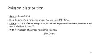
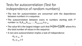
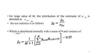
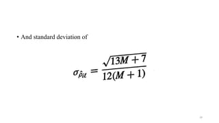
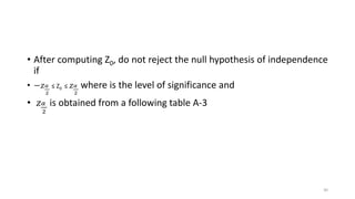
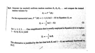
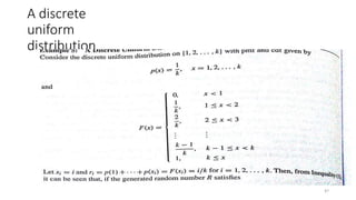
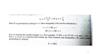
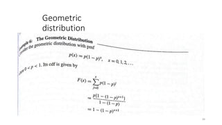
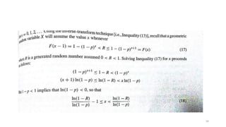
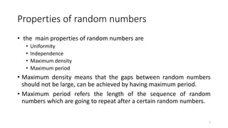
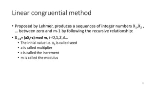
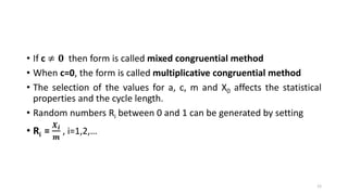
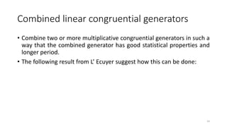
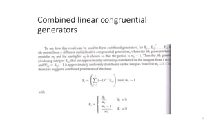
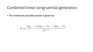
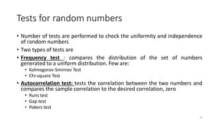
This document discusses random number generation and random variate generation. It covers: 1) Properties of random numbers such as uniformity, independence, maximum density, and maximum period. 2) Techniques for generating pseudo-random numbers such as the linear congruential method and combined linear congruential generators. 3) Tests for random numbers including Kolmogorov-Smirnov, chi-square, and autocorrelation tests. 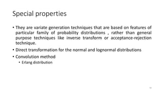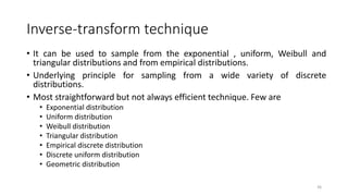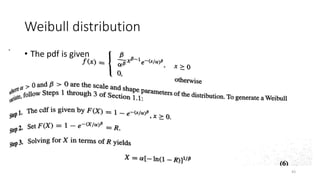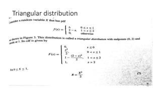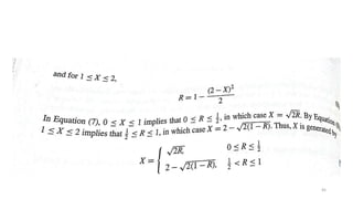4) Random variate generation techniques like the inverse transform method, acceptance-rejection technique, and special properties for distributions like normal, lognormal, and Erlang.

1. Random-Number Generation,
Random-Variate Generation
Unit 3

2. contents
• Random number generation
• Properties of random numbers
• Generation of pseudo-random numbers
• Techniques for generating random numbers
• Tests for Random Numbers
• Random-Variate Generation:
• Inverse transform technique
• Acceptance-Rejection technique
• Special properties
2

3. Random-Number Generation

4. Properties of random numbers
• the main properties of random numbers are
• Uniformity
• Independence
• Maximum density
• Maximum period
• Maximum density means that the gaps between random numbers
should not be large, can be achieved by having maximum period.
• Maximum period refers the length of the sequence of random
numbers which are going to repeat after a certain random numbers.
4

5. • Each random number Ri must be an independent sample drawn from
a continuous uniform distribution between zero and 1
• The pdf of the given by
• f(x)=
1 , 0 ≤ 𝑥 ≤ 1
0, 𝑜𝑡ℎ𝑒𝑟𝑤𝑖𝑠𝑒
• The expected value of each is given by
• E( R) = 0
1
𝑥 𝑑𝑥 =
1
2
5

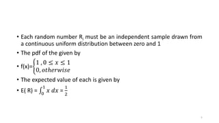
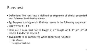
6. • The variance is given by
• V( R) = 0
1
𝑥2
− [𝐸 𝑅 ]2
=
1
12
• The following figure shows the pdf for random numbers
6

7. Generation of pseudo Random Numbers
• Pseudo means false , here it implies generating random numbers by
known method to remove the potential for true randomness.
• If the method is known then set of random numbers can be repeated.
• Which means that numbers are not random
• The main goal of random generation technique is to produce a
sequence of numbers between 0 and 1 that simulates or imitates the
ideal properties of uniform distribution and independence
• Random numbers are generated by digital computer as part of
simulation, there are numerous ways to generate these values
7

8. • The following are few important considerations
• The method should be fast, simulation process requires millions of random
numbers hence it has to be fast
• The method has to be portable to different computer
• The method should have sufficiently long cycle, means there should be long
gap between the random numbers once generated getting repeated.
• The random numbers should be repeatable
• The generated random numbers should closely approximate the ideal
statistical properties of uniformity and independence
8

9. Errors or departures of pseudo random
numbers
• The generated random numbers might not be uniformly distributed.
• Generated numbers might be discrete value instead of continuous
value.
• The mean of generated random numbers might be too high or too
low
• The variance of generated numbers might be too high or too low
• There might be dependence
• Authentication between numbers
• Numbers successively higher or lower than adjacent numbers
• Several numbers above the mean followed by several numbers below the
mean.
9

10. Techniques for generating random numbers
• Linear congruential method
• Combined linear congruential generators
• Random number streams
10

11. Linear congruential method
• Proposed by Lehmer, produces a sequences of integer numbers X1,X2 ,
… between zero and m-1 by following the recursive relationship:
• X i+1= (aXi+c) mod m, i=0,1,2,3…
• The initial value i.e. x0 is called seed
• a is called multiplier
• c is called the increment
• m is called the modulus
11

12. • If c ≠ 𝟎 then form is called mixed congruential method
• When c=0, the form is called multiplicative congruential method
• The selection of the values for a, c, m and X0 affects the statistical
properties and the cycle length.
• Random numbers Ri between 0 and 1 can be generated by setting
• Ri =
𝑿 𝒊
𝒎
, i=1,2,…
12

13. examples
13

14. Combined linear congruential generators
• Combine two or more multiplicative congruential generators in such a
way that the combined generator has good statistical properties and
longer period.
• The following result from L’ Ecuyer suggest how this can be done:
14

15. Combined linear congruential
generators
15

16. Combined linear congruential generators
• The maximum possible period is given by
16

17. examples
17

18. Tests for random numbers
• Number of tests are performed to check the uniformity and independence
of random numbers
• Two types of tests are
• Frequency test : compares the distribution of the set of numbers
generated to a uniform distribution. Few are:
• Kolmogorov-Smirnov Test
• Chi-square Test
• Autocorrelation test: tests the correlation between the two numbers and
compares the sample correlation to the desired correlation, zero
• Runs test
• Gap test
• Pokers test
18

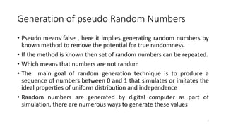
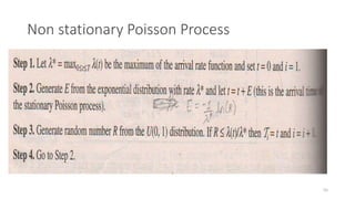
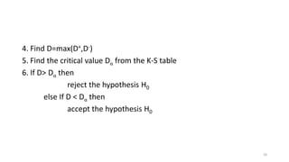
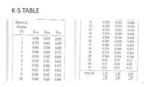
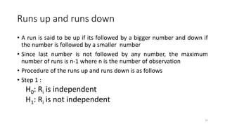
19. Kolmogorov- Smirnov Test –for uniformity (Procedure)
1. Formulate the hypothesis
H0:Ri ~U[0,1]
H1:Ri ~U[0,1]
2. Rank the data from smallest to largest
R(1)≤R(2) ≤R(3)…
3. Calculate the values of D+ and D-
19

20. 4. Find D=max(D+,D-)
5. Find the critical value Dα from the K-S table
6. If D> Dα then
reject the hypothesis H0
else If D < Dα then
accept the hypothesis H0
20

21. K-S TABLE
21

22. examples
22

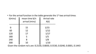
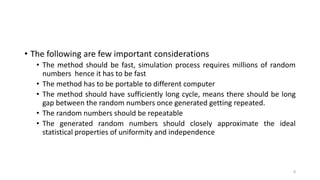
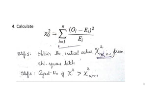
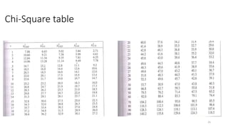
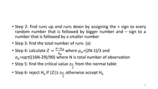
23. Chi-square Test –for uniformity (Procedure)
1. Formulate the hypothesis
H0:Ri ~U[0,1]
H1:Ri ~U[0,1]
2. Divide the data into different class intervals of equal intervals
3. Find out how many random numbers lie in each interval and hence find Oi
(observed frequency) & expected frequency Ei using the formula
Ei =
𝑁
𝑛
where N is the total no of observation
n is the no of class interval
L=n-1 is known as degree of freedom
23

24. 4. Calculate
24

25. Chi-Square table
25

26. examples
26

27. Tests for autocorrelation (Test for
independence of random numbers)
• The test for autocorrelation are concerned with the dependence
between numbers in a sequence.
• The autocorrelation between every m numbers starting with ith
number i.e. Ri,Ri+m,Ri+2m, … , Ri+(m+1)m is ρ im
• The value M is the largest integer such that i+(m+1)≤N where N is
the total number of values in the sequence
• A non-zero autocorrelation implies a lack of independence
H0: ρ im = 0
H1: ρ im ≠ 0
27

28. • For large value of M, the distribution of the estimator of ρ im is
denoted as ρ im
• the test statistics is as follows
• Which is distributed normally with a mean of 0 and variance of
28

29. • And standard deviation of
29

30. • After computing Z0, do not reject the null hypothesis of independence
if
• −𝑧 𝛼
2
≤ Z0 ≤ 𝑧 𝛼
2
where is the level of significance and
• 𝑧 𝛼
2
is obtained from a following table A-3
30

31. Runs test
• Definition: The runs test is defined as sequence of similar preceded
and followed by different events
• Eg. Suppose tossing a coin 10 times results in the following sequence
• H H T T T H T H T T
• Here are 6 runs, first one of length 2, 2nd length of 3, 3rd ,4th ,5th of
length 1 and 6th of length 2
• Two points to be considered while performing runs test
• No of runs
• Length of each run
31

32. Runs up and runs down
32
• A run is said to be up if its followed by a bigger number and down if
the number is followed by a smaller number
• Since last number is not followed by any number, the maximum
number of runs is n-1 where n is the number of observation
• Procedure of the runs up and runs down is as follows
• Step 1 :
H0: Ri is independent
H1: Ri is not independent

33. • Step 2: find runs up and runs down by assigning the + sign to every
random number that is followed by bigger number and – sign to a
number that is followed by a smaller number
• Step 3: find the total number of runs (a)
• Step 4: calculate 𝑍 =
𝑎−𝜇 𝑎
𝜎 𝑎
where 𝜇 𝑎=(2N-1)/3 and
𝜎 𝑎=sqrt((16N-29)/90) where N is total number of observation
• Step 5: find the critical value 𝑧 𝛼
2
from the normal table
• Step 6: reject H0 if |Z|≥ 𝑧 𝛼
2
otherwise accept H0
33

34. examples
34

35. Random-Variate Generation

36. Inverse-transform technique
• It can be used to sample from the exponential , uniform, Weibull and
triangular distributions and from empirical distributions.
• Underlying principle for sampling from a wide variety of discrete
distributions.
• Most straightforward but not always efficient technique. Few are
• Exponential distribution
• Uniform distribution
• Weibull distribution
• Triangular distribution
• Empirical discrete distribution
• Discrete uniform distribution
• Geometric distribution
36

37. Exponential distribution
• Probability density function (pdf) is given by
• 𝑓 𝑥 = λ𝑒−λ𝑥 , 𝑥 ≥ 0
0, 𝑥 < 0
• The cumulative distribution function (cdf) is given by
• F(x)= −∞
𝑥
𝑓 𝑡 𝑑𝑡 = 1 − 𝑒−λ𝑥, 𝑥 ≥ 0
0 , 𝑥 < 0
37

38. Procedure for inverse transform technique
38

39. 39

40. 40

41. examples
41

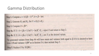
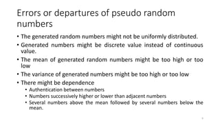
42. Uniform distribution
• Consider a random variable X i.e. uniformly distributed on the interval
[a,b].
• Step 1 : the cdf is given by
F(x) =
0, 𝑥 < 𝑎
𝑥−𝑎
𝑏−𝑎
, 𝑎 ≤ 𝑥 ≤ 𝑏
1, 𝑥 > 𝑏
• Step 2: Set F(x)=
𝑥−𝑎
𝑏−𝑎
= R
• Step 3: on solving we get , X=a+(b-a)R which is the equation for
random variate generation using uniform distribution
42

43. Weibull distribution
• The pdf is given
43

44. Triangular distribution
44

45. 45

46. examples
46

47. A discrete
uniform
distribution
47

48. 48

49. Geometric
distribution
49

50. 50

51. 51

52. Acceptance – rejection technique
• Devising a method for generating random numbers ‘X’ uniformly
distributed between ¼ and 1 follows three steps
1. Generate a random number R
2. a) If R ≥ ¼ accept X=R the goto step 3
2. b) if R < ¼ reject R and return to step 1
3. If another uniform random variate on [1/4,1] is needed, repeat the
procedure beginning at step 1 , if not stop.
52

53. Poisson distribution
• Step 1 : Set n=0, P=1
• Step 2 : generate a random number Rn+1 , replace P by P.Rn+1
• Step 3: If P < 𝑒−𝛼
then accept N=n, otherwise reject the current n, increase n by
one and return to step 2
• With N=n poison of average number is given by
E(N+1)=α+1
53

54. examples
54

55. Non stationary Poisson Process
55

56. • For the arrival function in the table generate the 1st two arrival times
t(mins) mean time b/n Arrival rate
arrival (mins) A(t)
0 15 1/15
60 12 1/12
120 17 1/17
180 5 1/5
240 8 1/8
300 10 1/10
Given the random no’s are: 0.2130, 0.8830, 0.5530, 0.0240, 0.0001, 0.1443
56

57. Gamma Distribution
57

58. Special properties
• They are variate generation techniques that are based on features of
particular family of probability distributions , rather than general
purpose techniques like inverse transform or acceptance-rejection
technique.
• Direct transformation for the normal and lognormal distributions
• Convolution method
• Erlang distribution
58

59. Direct transformation for the normal and
lognormal distributions
• The standard normal cdf is given by
ɸ (x) = −∞
𝑥 1
√2𝜋
𝑒
𝑡2
2 𝑑𝑡 , −∞ < 𝑥 < ∞
59

60. Convolution method
• The probability distribution of a sum of two or more independent
random variable is called convolution of distribution of the original
variable
• The convolution method refers to adding together two or more
random variables to obtain a new random variable with a desired
distribution
60

61. Erlang distribution
61

62. End of unit 3
Thank you 
62