The document provides an overview of the Craig-Bampton method for model reduction in finite element analysis. It discusses: - The background and theory behind the Craig-Bampton method, including defining the Craig-Bampton transformation matrix and deriving the reduced Craig-Bampton mass and stiffness matrices. - The process for creating a Craig-Bampton model in NASTRAN, including defining the boundary degrees of freedom, solving for modes, and generating the output files. - Different load transformation matrices (LTMs) that can be created, such as for interface forces, net center of gravity accelerations, and displacements, and how they are used to transform results between the reduced and full physical models.

1. The Craig-Bampton Method
FEMCI Presentation
Scott Gordon
May 6, 1999
Topics:
1) Background
2) Theory
3) Creating a C-B Model
4) Load Transformation Matrices
5) Verification
Appendix: Sample FLAME scripts

2. Background
• Who is Craig Bampton?
“Coupling of Substructures for Dynamic Analysis”
Roy R. Craig Jr. and Mervyn C. C. Bampton
AIAA Journal
Vol. 6, No. 7, July 1968
• What is the Craig-Bampton Method?
– Method for reducing the size of a finite element model.
– Combines motion of boundary points with modes of the structure assuming the
boundary points are held fixed
– Similar to other reduction schemes
•{U} = [φ]{Ua} Where [φ] = -[Koo]-1[Koa]
Guyan Reduction
{Ua} = A-set points
•{U} = [φ]{q} Where [φ] = Mode Shapes
Modal Decoupling
{q} = Modal dof’s
C-B Method
•{U} = [φ]{xcb} Where [φ] = C-B Transformation
{xcb} = C-B Dof’s =
boundary + modes
Scott Gordon
The Craig-Bampton
Page 2

3. Background (Cont)
• Why is the C-B Method Used?
–
–
–
–
Allows problem size to be reduced
Accounts for both mass and stiffness (unlike Guyan reduction)
Problem size defined by frequency range
Allows for different boundary conditions at interface (unlike
modal decoupling)
– Example
• Spacecraft Model:
10,000 DOF’s
K,M = 10,000 x 10,000
10 Modes up to 50 Hz
Single Boundary grid at interface
• C-B Reduction:
to 50 Hz
Scott Gordon
16 DOF (6 i/f + 10 Modes)
K,M = 16 x 16
The Craig-Bampton
Page 3

4. Craig-Bampton Theory
• Equation of motion (ignoring damping)
[ M ]{ u } + [ K ]{ u } = { F (t )}

AA
AA
A
A
(1)
• The Craig-Bampton transform is defined as:
u   I 0  u 
( 2)
{u } =   = 
 
φ φ  q 

u  
Where
C-B Transformation Matrix = φ
u = boundary dof's
u = internal (leftover) dof's
φ = Rigid body vector
φ = Fixed base modeshapes
q= modal dof's
b
b
A
L
R
L
cb
b
L
R
L
Scott Gordon
The Craig-Bampton
Page 4

5. Craig-Bampton Theory (Cont.)
• Combining equations (1) & (2) and pre-multiplying by [φcb]T

u 
u 
F 
φ [ M ]φ   + φ [ K ]φ   = φ  

q 
q 
F 
T
b
AA
cb
b
T
cb
AA
cb
(3)
b
T
cb
cb
L
• Define the C-B mass and stiffness matrices as
[
M
= φ [ M ]φ = 
M ]
M
K
[ K ] = φ [ K ]φ =  0

bb
T
cb
AA
cb
qb
cb
cb
qq
bb
AA
( 4)
bq
cb
T
M 
M 

0
K 

cb
(5)
qq
• Write equation (3) using equations (4) & (5)
M  u   K
0  u   F 

M
(6)
 +
 = 
M
M  q   0 K  q   0 





where input forces are applied at the boundary only (F = 0)
bb
bq
qb
qq
b
bb
b
b
qq
L
Scott Gordon
The Craig-Bampton
Page 5

6. Craig-Bampton Theory (Cont.)
• Important properties of the C-B mass and stiffness matrices
– Mbb = Bounday mass matrix => total mass properties translated to the
boundary points
[ M ] = φ [ M ]φ
(7 )
cg
cg T
RB
cg
bb
RB
– Kbb = Interface stiffness matrix => stiffness associated with displacing
one boundary dof while other are held fixed
• If the boundary point is a single grid (i.e. non-redundant) then
Kbb = 0
– If the mode shapes have been mass normalized (typically they are) then

0


K qq =  λ 
0




0


M qq =  I

0



Scott Gordon
λi = k i / mi = ω i2
The Craig-Bampton
(8)
Page 6

7. Craig-Bampton Theory (Cont.)
• We can finally write the dynamic equation of motion
(including damping) using the C-B transform as
M
M

M  u  0
0  u   K
0  u   F 


 +
 +
 = 
I   q  0 2ζω   q   0 ω   q   0 







where 2ζω = Modal damping (ζ=%critical)
bb
bq
b
b
bb
b
2
b
( 9)
qb
• Summary of C-B Theory
– C-B Mass and Stiffness Matrices fully define system
– Dynamics problem solved using CB dof’s
– C-B boundary dofs provide location to apply BC’s & Forces or to
couple with another structure
– CB transform is used to calculate physical responses from CB
responses
Scott Gordon
The Craig-Bampton
Page 7

8. How to Create a C-B Model
assign USER1=gi_v2_cb.kmnp,NEW,USE=OUTPUT4,TYPE=BINARY,reallocate  1) CB Output File
ID GLAST,inst
 2) Normal Modes Solution
SOL 3
APP DISP
TIME 5
$
 3) C-B DMAP
INCLUDE '/home/sag721/dmap/uai/cb_v118b.dmp'
CEND
$
TITLE = GLAST SI Instrument
SUBTITLE = Craig-Bampton Run
ECHO = NONE
METHOD = 1
$SPC = 998
$POST SDRC
DISP(NOPRINT)
=ALL
$SPCFORCES(NOPRINT)=ALL
$MPCFORCES(NOPRINT)=ALL
$
AUTOSPC = YES
BEGIN BULK
$
PARAM,GRDPNT,0
PARAM,WTMASS,2.59e-3
 4) Print G-set & R-set internal order
PARAM,USETPRT,0
$
 5) Define frequency range
EIGRL,1,-0.1,70.0
$
$ Instrument Interface at S/C
6) Boundary Defined on suport cards
SUPORT
800290
123456
SUPORT
800291
123456
8 boundary points x 6 dof’s
SUPORT
800292
123456
= 48 physical boundary points
SUPORT
800293
123456
SUPORT
800294
123456
SUPORT
800295
123456
SUPORT
800296
123456
SUPORT
800297
123456
$
 7) Don’t forget the rest of your bulk data
INCLUDE 'glast_inst_v2.blk'
$
ENDDATA
Scott Gordon
The Craig-Bampton
Page 8

9. How to Create a C-B Model (Cont.)
• What is created?
– file (.kmnp) which contains CB stiffness and mass matrices (k,m),
net CG ltm (n), and the CB transformation matrix (phig)
– .kmnp file is in NASTRAN binary output4 format
– K&M size is [CB dofs (boundary + modal) x CB dofs]
– phig size is [G-set rows x CB dofs]
– Net CG LTM recovers CG accelerations and I/F Forces, Size is
[6+boundary dofs x CB dofs]
• How do you use this?
– Solve dynamics problem for CB dof response using the K & M
matrices
– Transform CB responses using phig to get physical responses
Scott Gordon
The Craig-Bampton
Page 9

10. Load Transformation Matrices (LTMs)
• LTM is a generic term referring to the matrix used to
transform from CB dofs to physical dofs (also referred to
at OTMs, ATMs, DTMs…)
• In its simplest form, the LTM is simply the phig matrix
u

 } = [ φ ]  
{U
 

q
b
G
cb
(10)
(Only the rows corresponding to the physical dofs of interest are needed)
• There are other useful LTMs that can be created
– I/F forces
– Net CG accelerations
– Stress & force LTMs
Scott Gordon
The Craig-Bampton
Page 10

11. LTM’s (Cont.)
• I/F Force LTM (created by CB dmap)
I/F Force = [ M

u 
 
K ] q 
u 
 
b
M
bb
bq
(11)
bb
b
(If boundary is non-redundant, then Kbb=0)
• Net CG LTM (created by CB dmap)
Net CG Accel = ([φ
] [ M ][φ ] ) [φ ] [ M
CG T
rb
CG
bb
rb
−1
CG
rb
x
  
 

K ] q 
x 
 
b
T
bb
M
bq
bb
(12)
b
where
([φ
] [ M ][φ ] ) = mass matrix about cg (6x6)
[φ ] = rigid body transform from I/F to CG (bdof x6)
CG
rb
T
CG
bb
rb
CG
rb
Scott Gordon
The Craig-Bampton
Page 11

12. LTM’s (Cont.)
• PHIZ LTM
– Allows physical displacements to be calculated from CB
accelerations

x 
{ X } = [ PHIZ ]  
q
b
G
  
(13)
– Same as modal acceleration approach in NASTRAN
– Useful in calculating relative displacements between DOF’s
– Also used to calculate stresses and forces which are a function of
displacements
– Calculated from C-B dmap using => param,phzout,1
Scott Gordon
The Craig-Bampton
Page 12

13. LTM’s (Cont.)
• LTM’s can be created using FLAME, MATLAB or using
DMAP
• LTM’s can (and usually do) contain multiple types of
 [ Net CG ] 
responses


[ I / F Force] 
LTM =  [ Accel ] 
 Element 
 
 
  Forces  
 
 
(14)
• LTM’s can be used to recover responses for nested C-B

models { X } = [ φ ][ φ ] x 
(15)
 
cb1
cb1
cb
where φcb 01
cb1
cb 0
cb 0
b
cb 0
q 
= row partition of the CB1 Dofs from the CB0 PHIG Matrix
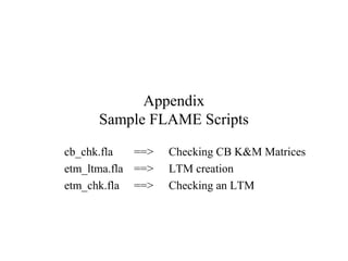
• Creating LTMs - See appendix for a sample FLAME script
for creating an LTM
Scott Gordon
The Craig-Bampton
Page 13

14. Checking CB Models & LTM’s
• C-B Models and LTMs should be verified to make sure
that they have been created correctly (especially for
complicated LTM’s or nested C-B models)
• CB Mass and stiffness matrices can be checked by
computing free-free and fixed-base modes
• CB boundary Mass matrix can be transformed to CG and
compared with NASTRAN GPWG
Scott Gordon
The Craig-Bampton
Page 14

15. Checking C-B Models and LTM’s (Cont.)
• LTMS can be checked by applying unit acceleration at the boundary
LTM
b q φ
{ X } =     (16)

 0 

 
where φ = Boundary rigid body vector (b x 6)
b
RB
resp
b
RB
–
–
–
–
Each response column represents acceleration in a single direction
Accelerations should be in correct directions
Forces should recover weight or correct moments
Unit acceleration applied to PHIZ can be checked by gravity run with
physical model and comparing displacements
• See appendix for sample FLAME scripts to check a CB model and
LTM
Scott Gordon
The Craig-Bampton
Page 15

16. Appendix
Sample FLAME Scripts
cb_chk.fla
==>
etm_ltma.fla ==>
etm_chk.fla ==>
Checking CB K&M Matrices
LTM creation
Checking an LTM