This document provides an overview of a computational materials science lecture at Tokyo Tech. The lecture will cover first principles calculations, focusing on numerical analysis of electronic states. First principles calculations determine electronic states without experimental parameters by only using fundamental physical constants and numerical parameters. The lecture notes can be downloaded online and questions are welcome. Example materials that will be discussed include graphene and magnetic materials interfaces. Computational methods like density functional theory and plane wave basis sets will be introduced.

1. 計算材料学
Computational Materials Science
東京工業大学大学院総合理工学研究科2014 年度冬学期
Tokyo Tech Winter Semester, AY2014
October 17, 2014
合田義弘
Y. Gohda
はじめに/Introduction
計算機を用いたシミュレーションは実験と相補的な立場にある材料学研究に欠かせないツールで
ある。本講義の内、合田担当分では第一原理計算を中心に電子状態の数値解析について扱う。第
一原理計算とは、実験的に決定されたパラメーターを用いず、素電荷e、Planck 定数! 等の基礎
的な物理定数と計算精度をコントロールする数値解析的パラメーターのみによる非経験的電子状
態計算の事である。
この講義ノートは
http://www.cms.materia.titech.ac.jp/lecture_cms.pdf
においてダウンロード可能である（要パスワード）。質問は歓迎する。講義中にどんどんしてほし
い。参考書としては
押山淳ほか：岩波講座計算科学3 「計算と物質」
R.M. Martin: Electronic Structure 日本語訳あり
J.M. ティッセン：「計算物理学」
J.J. Sakurai: Modern Quantum Mechanics 日本語訳あり
を勧める。
第一原理計算を実際に試す事も可能である。Mac あるいはLinux にコードを自分でインストー
ルしても良いが、“MateriApps LIVE!” のUSB を入手あるいは作成すれば、手持ちのコンピュー
ターで計算環境が整備済のLinux をUSB ブートする事が出来る。“MateriApps LIVE!” に収録さ
れているOpenMX コードを勧める。
東京工業大学の国際化推進に向けた方針に鑑み、以下の講義ノートは原則英語で記述する。
1

2. Contents
1 Born-Oppenheimer approximation and many-electron system 3
1.1 Summary of basic quantum mechanics . . . . . . . . . . . . . . . . . . . . . . . . 3
1.2 Born-Oppenheimer approximation . . . . . . . . . . . . . . . . . . . . . . . . . . 4
1.3 Molecular dynamics and structure optimization. . . . . . . . . . . . . . . . . . . . 6
1.4 Quantum many-body theory of electrons . . . . . . . . . . . . . . . . . . . . . . . 9
2 Hartree-Fock approximation and wave-function theory 12
2.1 Hartree-Fock approximation . . . . . . . . . . . . . . . . . . . . . . . . . . . . . . 12
2.2 Post-Hartree-Fock . . . . . . . . . . . . . . . . . . . . . . . . . . . . . . . . . . . 16
2.3 Diffusion Monte Carlo Method . . . . . . . . . . . . . . . . . . . . . . . . . . . . 18
3 Density functional theory 21
3.1 Hohenberg–Kohn theorem and the Kohn-Sham equation . . . . . . . . . . . . . . 21
3.2 Exchange-correlation functionals . . . . . . . . . . . . . . . . . . . . . . . . . . . 23
3.3 Beyond standard DFT . . . . . . . . . . . . . . . . . . . . . . . . . . . . . . . . . 25
4 Basis sets 28
4.1 Without basis sets: real-space discretization . . . . . . . . . . . . . . . . . . . . . 28
4.2 Plane-wave basis . . . . . . . . . . . . . . . . . . . . . . . . . . . . . . . . . . . . 28
4.3 Pseudo-atomic orbitals as a basis set . . . . . . . . . . . . . . . . . . . . . . . . . 29
5 Examples 33
5.1 Diatomic molecules: N2 and O2 . . . . . . . . . . . . . . . . . . . . . . . . . . . . 33
5.2 Graphene . . . . . . . . . . . . . . . . . . . . . . . . . . . . . . . . . . . . . . . . 34
5.3 Microstructure interfaces of magnetic materials . . . . . . . . . . . . . . . . . . . 41
2

3. 5.2 Graphene
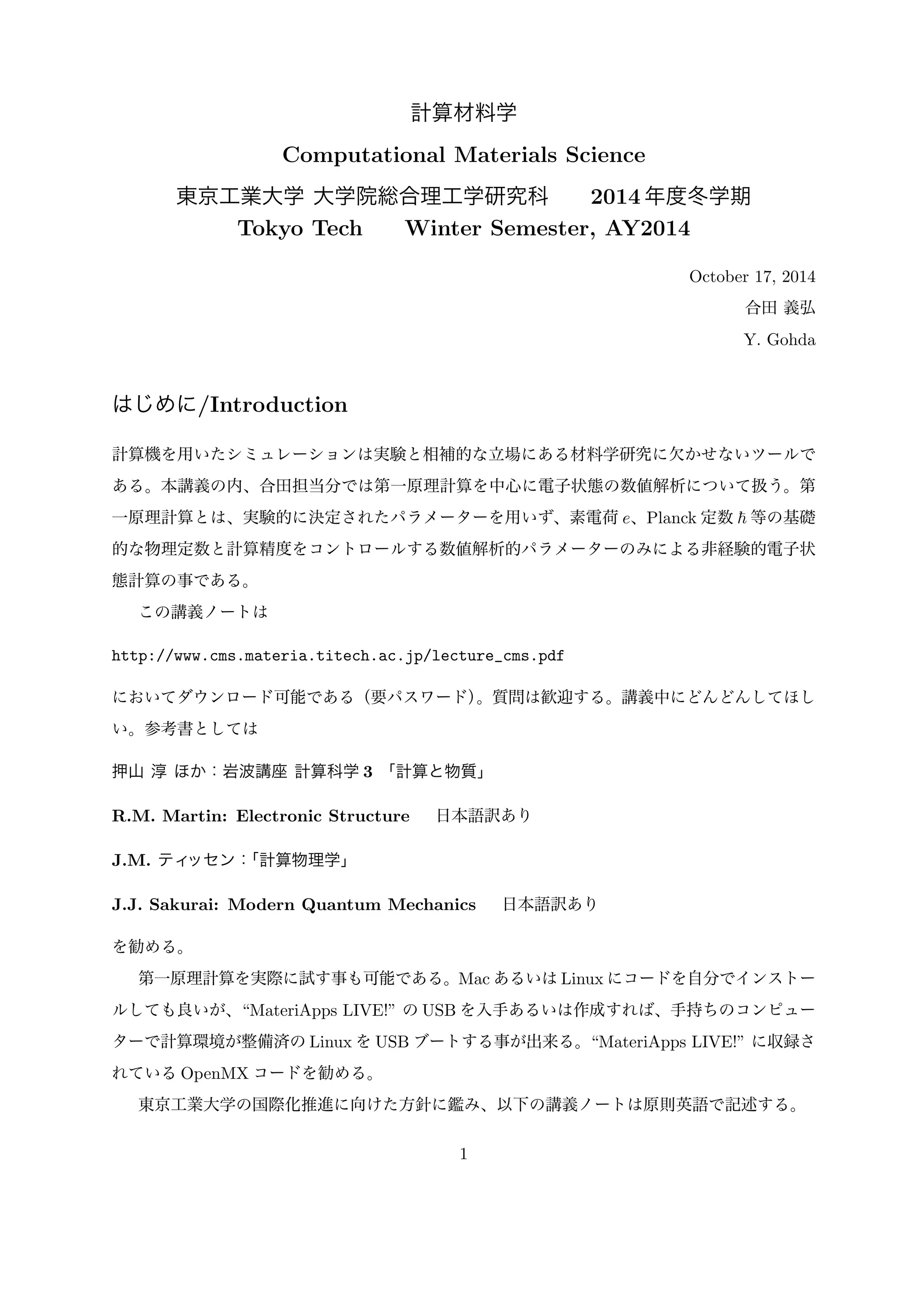
Brillouin zone of the hexagonal lattice
lattice vectors:
a = a
!
1
2
ex −
√3
2
ey
"
, b = a
!
1
2
ex +
√3
2
ey
"
, c = cez .
reciprocal-lattice vectors:
Ga = 2π
b × c
a · (b × c)
=
4π
√3a2c
b × c =
4π
√3a
!√3
2
ex −
1
2
ey
"
,
Gb = 2π
c × a
a · (b × c)
=
4π
√3a2c
c × a =
4π
√3a
!√3
2
ex +
1
2
ey
"
,
Gc = 2π
a × b
a · (b × c)
=
4π
√3a2c
a × b =
2π
c
ez .
Γ: Center of the Brillouin zone
K: Middle of an edge joining two rectangular faces→ (Ga + Gb)/3
M: Center of a rectangular face → Ga/2
A: Center of a hexagonal face → Gc/2
H: Corner point → (Ga + Gb)/3 + Gc/2
L: Middle of an edge joining a hexagonal and a rectangular face → Ga/2 + Gc/2
10
5
0
−5
Energy relative to EF [eV]
−10
Γ KM Γ A H L Γ
Figure 6: Band structure of the normal state
of a superconductor, MgB2.
34

4. Unit cell and atomic structure of graphene
The computational cell for graphene is hexagonal one.
(a) (b)
Figure 7: The unit cell and the atomic struc-ture
of graphene used for first-principles calcu-lations:
(a) the side view and (b) the top view.
Input file of OpenMX to calculate electronic states of graphene
#
# OpenMX Inputfile
#
# File Name
#
System.Name graphene
DATA.PATH /home/gohda/openmx/DFT_DATA13
# Definition of Atomic Species
#
Species.Number 2
<Definition.of.Atomic.Species
C C6.0-s2p2d1 C_PBE13
E Rn13.0-s2p2d2f1 E
Definition.of.Atomic.Species>
# Atoms
#
Atoms.Number 3
Atoms.SpeciesAndCoordinates.Unit FRAC # Ang|AU
<Atoms.SpeciesAndCoordinates
1 C 0.33333333333333 0.66666666666667 0.50000000000000 2.0 2.0
2 C 0.66666666666667 0.33333333333333 0.50000000000000 2.0 2.0
3 E 0.00000000000000 0.00000000000000 0.50000000000000 0.0 0.0
Atoms.SpeciesAndCoordinates>
35

5. Atoms.UnitVectors.Unit Ang # Ang|AU
<Atoms.UnitVectors
1.23000000000000 -2.13042249330972 0.00000000000000
1.23000000000000 2.13042249330972 0.00000000000000
0.00000000000000 0.00000000000000 10.00000000000000
Atoms.UnitVectors>
# SCF or Electronic System
#
scf.XcType GGA-PBE # LDA|LSDA-CA|LSDA-PW|GGA-PBE
scf.SpinPolarization off # On|Off|NC
scf.energycutoff 300.0 # default=150 (Ry)
scf.maxIter 100 # default=40
scf.EigenvalueSolver band # DC|GDC|Cluster|Band
scf.Kgrid 11 11 1 # means n1 x n2 x n3
scf.Mixing.Type rmm-diisk # Simple|Rmm-Diis|Gr-Pulay|Kerker|Rmm-Diisk
scf.Init.Mixing.Weight 0.30 # default=0.30
scf.Min.Mixing.Weight 0.001 # default=0.001
scf.Max.Mixing.Weight 0.700 # default=0.40
scf.Mixing.History 10 # default=5
scf.Mixing.StartPulay 5 # default=6
scf.Mixing.EveryPulay 1 # default=5
scf.criterion 1.0e-6 # default=1.0e-6 (Hartree)
scf.lapack.dste dstevx # dstegr|dstedc|dstevx, default=dstevx
# DOS and PDOS
#
Dos.fileout on # on|off, default=off
Dos.Erange -20.0 10.0 # default = -20 20
Dos.Kgrid 48 48 1 # default = Kgrid1 Kgrid2 Kgrid3
# Band dispersion
#
Band.dispersion on # on|off, default=off
Band.Nkpath 4
<Band.kpath
200 0.0 0.0 0.0 0.33333333333333 0.33333333333333 0.0 G K
100 0.33333333333333 0.33333333333333 0.0 0.5 0.0 0.0 K M
173 0.5 0.0 0.0 0.0 0.0 0.0 M G
37 0.0 0.0 0.0 0.0 0.0 0.5 G A
Band.kpath>
# Others
#
scf.restart on
scf.fixed.grid 0.00000000000000 0.00000000000000 0.00000000000000
36

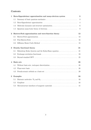
6. Band strucuture and density of states
You can excecute OpenMX by typing on a UNIX (MacOSX, Linux, etc.) terminal as follows:
$ openmx INCAR >log 2>&1 &
5
(a) (b)
0
−10
Γ K M Γ A
−5
Energy relative to EF [eV]
−15
−20
0
−20 −15 −10 −5 0 5 10
Energy relative to EF [eV]
Density of states [arb. unit]
w EA
w/o EA
w EA
w/o EA
(c)
Figure 8: (a) The energy band and (b) the de-sity
of states for graphene obtained by first-principles
calculations with enpty-atom basis
functions (red) and without them (black). (c)
Nearly-free-electron states that cannot be de-scribed
without the empty atom.
Comparison with the tight-binding model with the H¨uckel approximation
In the Huckel ¨approximation, only the |φpz ⟩ state is considered for the frontier orbitals of benzene
rings. The tight-binding Hamiltonian using the notation of |I⟩ = |φI
pz ⟩ is
H =
#
I
εI |I⟩⟨I|−
#
<IJ>
t|I⟩⟨J| = −
#
<IJ>
t|I⟩⟨J| , (23)
where t is the transfer integral and we define εI = 0. Using the Bloch sum
φB
i,k(r) =
1
√Nk
#
T
eik·T φpz (r − Ri − T ) (24)
with the approximation of ⟨I|J⟩ = δIJ (Thus Sij = δij), the matrix elements are
⟨φB
i,k|H|φB
i,k⟩ = 0 , and (25)
⟨φB
i,k|H|φB
j,k⟩ = ⟨φB
i,k⟩∗ = −t(eik·T0 + eik·T1 + eik·T2)
j,k|H|φB
= −t(1 + eik·a + e−ik·b) ≡ −tf . (26)
37

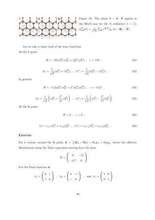
7. Thus the transformed Hamiltonian becomes
H = −t(f|φB1
⟩⟨φB2
| + f∗|φB2
⟩⟨φB1
|) . (27)
Diagonalizing H through ε2 − t2|f|2 = 0, we obtain
ε = ±t|f|
= ±t
$
(1 + cos k · a + cos k · b)2 + (sink · a − sin k · b)2
= ±t
$
3 + 2 cos k · a + 2 cos k · b + 2 cos k · (a + b) . (28)
At the M point (k = Ga/2),
ε = ±t
$
3 + 2 cos k · a + 2 cos k · b + 2 cos k · (a + b)
= ±t
$
5 + 4 cosGa/2 · a
= ±t√5 + 4 cos π
= ±t . (29)
As for the Γ–K path, i.e. k = κ(Ga + Gb),
ε = ±t
$
3 + 2 cos k · a + 2 cos k · b + 2 cos k · (a + b)
= ±t
$
3 + 2 cos κGa · a + 2 cos κGb · b + 2 cos κ(Ga + Gb) · (a + b)
= ±t
$
3 + 4 cos (2πκ) + 2 cos(4πκ) (30)
Γ K
10
5
0
Energy relative to EF [eV]
−5
w EA
w/o EA
TB
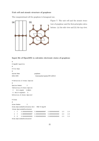
Figure 9: Comparison of energy bands ob-tained
by first-principles calculations and the
tight-binding model with the H¨uckel approxi-mation.
The hopping integral was chosen as
t = 2.7 eV.
38

8. Γ K M
0 0
0 0
0
0
0
0 0
0
0
π 0
π
π
0 0
π π
0
0
π
π
π
π
π
π
B1
Figure 10: The phase θ = k · T appear in
the Bloch sum for the A sublattice (i = 1),
%
φk(r) = √1 ,Nk
T eik·T φpz (r − R1 − T ).
Let us take a closer look of the wave functions:
At the Γ point:
H = −3t(|φB1
⟩⟨φB2
| + |φB2
⟩⟨φB1
|) , ε= ±3t , (31)
|π⟩ =
1
√2
(|φB1
⟩ + |φB2
⟩) , |π∗⟩ =
1
√2
(|φB1
⟩ − |φB2
⟩) . (32)
In general:
H = −t(f|φB1
⟩⟨φB2
| + f∗|φB2
⟩⟨φB1
|) , ε= ±t|f| , (33)
|π⟩ =
1
√2
&
|φB1
⟩ +
f∗
|f||φB2
⟩
'
, |π∗⟩ =
1
√2
&
|φB1
⟩ −
f∗
|f||φB2
⟩
'
. (34)
At the K point:
H = 0 , ε= 0 , (35)
|π⟩ = cπ,1|φB1
⟩ + cπ,2|φB2
⟩ , |π∗⟩ = cπ∗,1|φB1 ⟩ + cπ∗,2|φB2
⟩ . (36)
Exercise
For k vectors around the K point, k = 13
(Ga + Gb) + δkxex + δkyey, derive the effective
Hamiltonian using the Talor expansion starting from the form
H =
⎛
⎝ 0 −tf
−tf ∗ 0
⎞
⎠ .
Use the Pauli matrices σ:
σx =
⎛
⎝ 0 1
1 0
⎞
⎠ , σy
=
⎛
⎝ 0 −i
i 0
⎞
⎠ , and σz =
⎛
⎝ 1 0
0 1
⎞
⎠ .
39

9. Answer:
Exercise
Calculate i) the eigenenergy and ii) the sign of the linear combination for π orbitals in a butadiene
molecule CH2CHCHCH2, a virtual fragment of graphene, using the H¨uckel approximation.
Hint: 2 < √5 < 3
Answer:
40