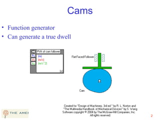
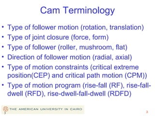
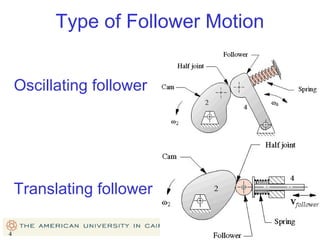
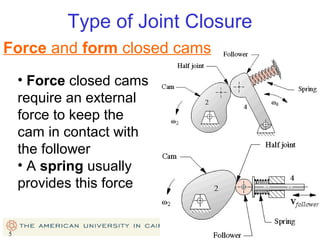
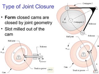
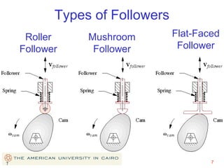
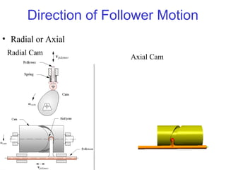
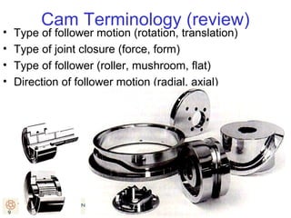
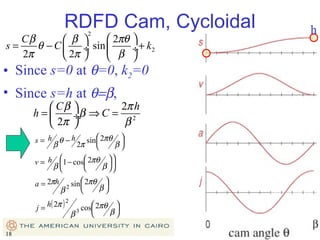
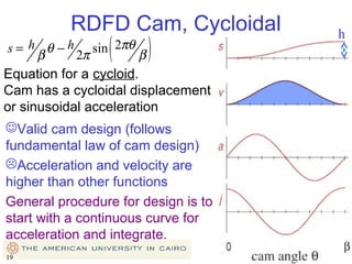
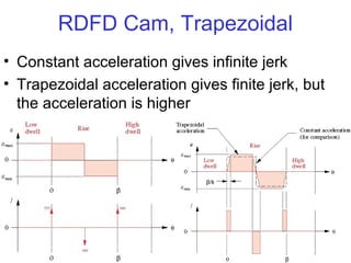
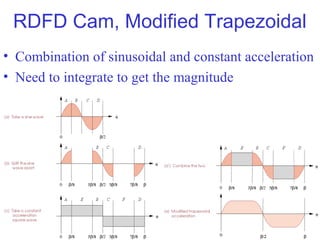
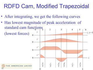
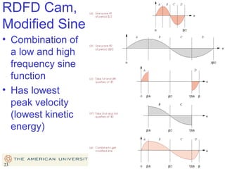
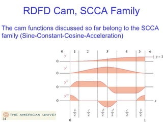
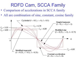
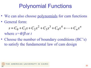
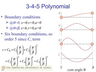
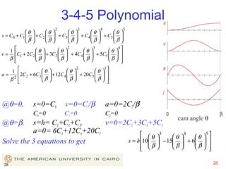
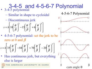
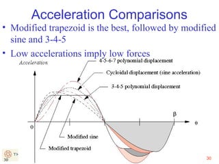
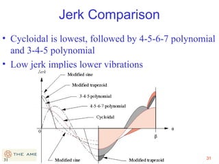
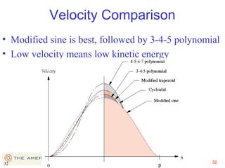
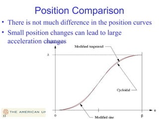
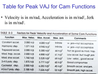
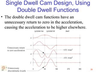
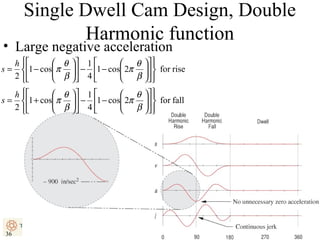
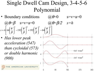
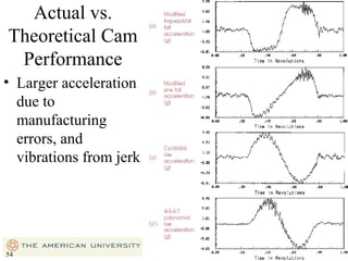
This document provides an overview of cam design principles and functions. It begins by defining different cam terminology such as follower motion types, joint closure types, follower types, and motion constraints. It then discusses common cam motion programs including rise-fall, rise-fall-dwell, and rise-dwell-fall-dwell. Several cam profile functions are analyzed that satisfy the fundamental law of cam design requiring continuous derivatives, including cycloidal, trapezoidal, and polynomial functions. Comparisons of the velocity, acceleration, jerk, and position profiles of different cam functions show that modified trapezoidal cams have the lowest peak acceleration while cycloidal and polynomial cams have the lowest jerk. The document concludes with considerations for single dwell cam design.

1. MENG 372
Chapter 8
Cam Design
All figures taken from Design of Machinery, 3rd ed. Robert Norton
2003
1
1

2. Cams
• Function generator
• Can generate a true dwell
2
2

3. Cam Terminology
•
•
•
•
•
Type of follower motion (rotation, translation)
Type of joint closure (force, form)
Type of follower (roller, mushroom, flat)
Direction of follower motion (radial, axial)
Type of motion constraints (critical extreme
position(CEP) and critical path motion (CPM))
• Type of motion program (rise-fall (RF), rise-falldwell (RFD), rise-dwell-fall-dwell (RDFD)
3
3

4. Type of Follower Motion
Oscillating follower
Translating follower
4
4

5. Type of Joint Closure
Force and form closed cams
• Force closed cams
require an external
force to keep the
cam in contact with
the follower
• A spring usually
provides this force
5
5

6. Type of Joint Closure
• Form closed cams are
closed by joint geometry
• Slot milled out of the
cam
6
6

7. Types of Followers
Roller
Follower
Mushroom
Follower
Flat-Faced
Follower
• Roller Follower
• Mushroom Follower
• Flat-Faced Follower
7
7

8. Direction of Follower Motion
• Radial or Axial
Radial Cam
8
Axial Cam
8

9. Cam Terminology (review)
•
•
•
•
Type of follower motion (rotation, translation)
Type of joint closure (force, form)
Type of follower (roller, mushroom, flat)
Direction of follower motion (radial, axial)
9
9

10. Type of Motion Constraints
• Critical Extreme Position (CEP) – start and end
positions are specified but not the path
between
• Critical Path Motion (CPM) – path or derivative
is defined over all or part of the cam
10
10

11. Type of Motion Program
• From the CEP cam profile
• Dwell – period with no output motion with input
motion.
• Rise-Fall (RF) – no dwell (think about using a
crank-rocker)
• Rise-Fall-Dwell (RFD) – one dwell
• Rise-Dwell-Fall-Dwell (RDFD) – two dwells
11
11

12. SVAJ Diagrams
• Unwrap the cam
• Plot position (s),
velocity (v),
acceleration (a) and
jerk (j) versus cam
angle
• Basis for cam design
12
12

13. RDFD Cam Design
• Motion is between two dwells
13
13

14. RDFD Cam, Naïve Cam Design
• Connect points using
straight lines
• Constant velocity
 Infinite acceleration
and jerk
 Not an acceptable
cam program
14
14

15. Fundamental Law of Cam Design
Any cam designed for operation at other than
very low speeds must be designed with the
following constraints:
• The cam function must be continuous through
the first and second derivatives of displacement
across the entire interval (360°).
Corollary:
• The jerk must be finite across the entire interval
(360°).
15
15

16. RDFD Cam Sophomore Design
Simple Harmonic Motion
• Sine function has
continuous derivatives
s=
 πθ
h
1 - cos 

2
 β
h

÷

 πθ 
ds hπ
=
sin 
÷
dθ 2 β
 β 
 πθ 
dv hπ 2
a=
=
cos 
dθ 2 β 2
β ÷


v=
 πθ 
da −hπ 3
j=
=
sin 
÷
dθ
2β 3
 β 
∞
∞
 Acceleration is discontinuous
 Jerk is infinite (bad cam design)
16
16

17. RDFD Cam, Cycloidal
Start with acceleration & integrate:
 2πθ 
a = C sin 
β ÷


 2πθ
Cβ
v=−
cos 
2π
 β
Since
k1 =
v=0
Cβ
2π
Cβ
v=
2π
at

÷+ k1

θ =0

 2πθ
1 − cos 
 β

h
then:

÷

2
 2πθ 
Cβ
 β 
s=
θ − C  ÷ sin 
÷+ k 2
2π
 2π 
 β 
17
17

18. RDFD Cam, Cycloidal
h
2
 2πθ 
Cβ
 β 
s=
θ − C  ÷ sin 
÷+ k 2
2π
 2π 
 β 
• Since s=0 at θ=0, k2=0
• Since s=h at θ=β,
 Cβ
h=
 2π
2π h

÷β ⇒ C = 2
β

s = h θ − h sin  2πθ 
β
2π 
β


v = h 1 − cos 2πθ  

β
β 



a = 2πh 2 sin  2πθ 

β


β
h( 2π ) 2
j=
18
β
 2πθ 
β


3 cos
18

19. RDFD Cam, Cycloidal
(
)
s = h θ − h sin 2πθ
β
2π
β
Equation for a cycloid.
Cam has a cycloidal displacement
or sinusoidal acceleration
h
Valid cam design (follows
fundamental law of cam design)
Acceleration and velocity are
higher than other functions
General procedure for design is to
start with a continuous curve for
acceleration and integrate.
19
19

20. RDFD Cam, Trapezoidal
• Constant acceleration gives infinite jerk
• Trapezoidal acceleration gives finite jerk, but
the acceleration is higher
20
20

21. RDFD Cam, Modified Trapezoidal
• Combination of sinusoidal and constant acceleration
• Need to integrate to get the magnitude
21
21

22. RDFD Cam, Modified Trapezoidal
• After integrating, we get the following curves
• Has lowest magnitude of peak acceleration of
standard cam functions
(lowest forces)
22
22

23. RDFD Cam,
Modified Sine
• Combination of
a low and high
frequency sine
function
• Has lowest
peak velocity
(lowest kinetic
energy)
23
23

24. RDFD Cam, SCCA Family
The cam functions discussed so far belong to the SCCA
family (Sine-Constant-Cosine-Acceleration)
24
24

25. RDFD Cam, SCCA Family
• Comparison of accelerations in SCCA family
• All are combination of sine, constant, cosine family
25
25

26. Polynomial Functions
• We can also choose polynomials for cam functions
• General form:
2
3
4
n
s = C0 + C1 x + C2 x + C3 x + C4 x +  + Cn x
where x=θ/β or t
• Choose the number of boundary conditions (BC’s)
to satisfy the fundamental law of cam design
26
26

27. 3-4-5 Polynomial
• Boundary conditions
 @θ=0, s=0,v=0,a=0
 @θ=β, s=h,v=0,a=0
• Six boundary conditions, so
order 5 since C0 term
θ 
θ
s = C0 + C1   + C2 
β
β
 

3
θ 
θ
+ C3   + C4 
β
β
 

27
4




2

θ 
 + C5  

β

 
5
27

28. 3-4-5 Polynomial
θ
s = C0 + C1 
β


θ
 + C2 

β


2
3
4

θ 
θ 
θ 
 + C3   + C4   + C5  

β
β
β

 
 
 
5
2
3
4
θ 
θ 
θ 
θ  
1
v = C1 + 2C2   + 3C3   + 4C4   + 5C5   
β 
β
β 
β
β
 
 
 
  


2
3
θ 
θ 
θ  
1 
a = 2 2C2 + 6C3   + 12C4   + 20C5   
β 
β 
β
β 
 
 
  


@θ=0,
@θ=β,
s=0=C0
v=0=C1/β
a=0=2C2/β2
C0=0
C1=0
C2=0
s=h= C3+C4+C5,
v=0=2C3+3C4+5C5
a=0= 6C3+12C4+20C5
  θ 3
θ
s = h 10  − 15
Solve the 3 equations to get
 

 β 

28
4
5

θ  
 + 6  

β
β 
  

28

29. 3-4-5 and 4-5-6-7 Polynomial
• 3-4-5 polynomial
– Similar in shape to cycloidal
– Discontinuous jerk
 θ
s = h 10

 β

3

θ
 − 15

β


4-5-6-7 Polynomial
5
4

θ 
 + 6  

β 

  

• 4-5-6-7 polynomial: set the jerk to be
zero at 0 and β
 θ
s = h 35

 β

4

θ
 − 84

β


5
6

θ 
θ
 + 70  − 20

β
β

 





7



• Has continuous jerk, but everything
else is larger
29
29

30. Acceleration Comparisons
• Modified trapezoid is the best, followed by modified
sine and 3-4-5
• Low accelerations imply low forces
30
30

31. Jerk Comparison
• Cycloidal is lowest, followed by 4-5-6-7 polynomial
and 3-4-5 polynomial
• Low jerk implies lower vibrations
31
31

32. Velocity Comparison
• Modified sine is best, followed by 3-4-5 polynomial
• Low velocity means low kinetic energy
32
32

33. Position Comparison
• There is not much difference in the position curves
• Small position changes can lead to large
acceleration changes
33
33

34. Table for Peak VAJ for Cam Functions
• Velocity is in m/rad, Acceleration is in m/rad 2, Jerk
is in m/rad3.
34
34

35. Single Dwell Cam Design, Using
Double Dwell Functions
• The double dwell cam functions have an
unnecessary return to zero in the acceleration,
causing the acceleration to be higher elsewhere.
35
35

36. Single Dwell Cam Design, Double
Harmonic function
• Large negative acceleration
 θ  1 
 θ  
h 


s = 1 − cos π  − 1 − cos 2π   for rise
 β 4
 β
2 



 



 θ  1 
 θ  
h 


s = 1 + cos π  − 1 − cos 2π   for fall
 β 4
 β
2 



 



36
36

37. Single Dwell Cam Design, 3-4-5-6
Polynomial
• Boundary conditions
@θ=β s=v=a=0
@θ=0
@θ=β/2
 θ
s = h 64

 β





3
4
• Has lower peak
acceleration (547)
than cycloidal (573)
or double harmonic
(900)
37
5

θ 
θ 
θ
 − 192  + 192  − 64

β
β
β

 
 

s=v=a=0
s=h
6



37

38. Unsymmetrical RFD Cams
• If the rise has different time than the fall, need more
boundary conditions.
• With 7BC’s
38
38

39. Unsymmetrical RFD Cams
• If you set the velocity to zero at the peak:
39
39

40. Unsymmetrical RFD Cams
• With 3 segments, segment 1 with 5BC’s, segment 2
with 6BC’s get a large peak acceleration
40
40

41. Unsymmetrical RFD Cams
• Best to start with segment with lowest acceleration
with 5BC’s then do the other segment with 6BC’s
41
41

42. Critical Path Motion (CPM)
• Position or one of its derivatives is specified
• Ex: Constant velocity for half the rotation
• Break the motion into the following parts:
42
42

43. Critical Path Motion (CPM)
• Segment 1 has
4BC’s
• Segment 2 has
2BC’s (constant V)
• Segment 3 has
4BC’s
• Last segment has
6BC’s (almost
always)
43
43

44. Resulting Curves
44
44

45. Constant Velocity, 2 Segments
• The divisions on the previous approach are not
given, only one segment of constant velocity
45
45

46. Resulting SVAJ diagram
• 2 segment design has better properties
• 4 segment design had ∆s=6.112, v=-29.4, a=257
46
46

47. Sizing the Cam, Terminology
• Base circle (Rb) – smallest circle that can be drawn
tangent to the physical cam surface
• Prime circle (Rp) – smallest circle that can be drawn
tangent to the locus of the centerline of the follower
• Pitch curve – locus
of the centerline of
the follower
47
47

48. Cam Pressure Angle
• Pressure Angle (φ)
– the angle between
the direction of
motion (velocity) of
the follower and the
direction of the axis
of transmission
• Want φ<30 for
translating and φ<35
for oscillating
followers
48
φ
48

49. Cam Eccentricity
• Eccentricty (ε) – the
perpendicular distance
between the follower’s
axis of motion and the
center of the cam
• Aligned follower: ε=0
49
ε
b
49

50. Overturning Moment
For flat faced follower,
the pressure angle is
zero
There is a moment on
the follower since the
force is not aligned
with the direction of
follower motion. This
is called the
overturning moment
50
50

51. Radius of Curvature
• Every point on the cam has an associated radius of
curvature
• If the radius of curvature is smaller than the radius of the
follower the follower doesn’t move properly
• Rule of thumb: ρmin =(2→3) x Rf
51
51

52. Radius of Curvature – Flat Faced
Follower
• We can’t have a negative
radius of curvature
52
52

53. Cam Manufacturing Considerations
•
•
•
•
53
Medium to high carbon steels, or cast ductile iron
Milled or ground
Heat treated for hardness (Rockwell HRC 50-55)
CNC machines often use linear interpolation (larger
accelerations)
53

54. Actual vs.
Theoretical Cam
Performance
• Larger acceleration
due to
manufacturing
errors, and
vibrations from jerk
54
54

55. Practical Design Considerations
• Translating or oscillating follower?
• Force or Form-Closed?
– Follower Jump vs. Crossover Shock
•
•
•
•
•
55
Radial or Axial Cam?
Roller or Flat-Faced Follower?
To Dwell or Not to Dwell?
To Grind or not to Grind?
To Lubricate or Not to Lubricate?
55