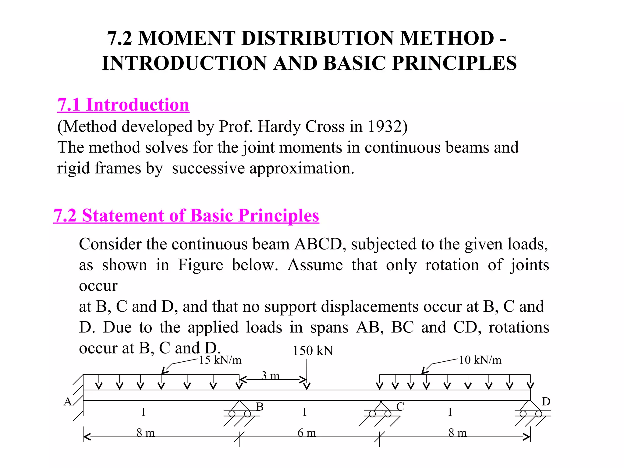
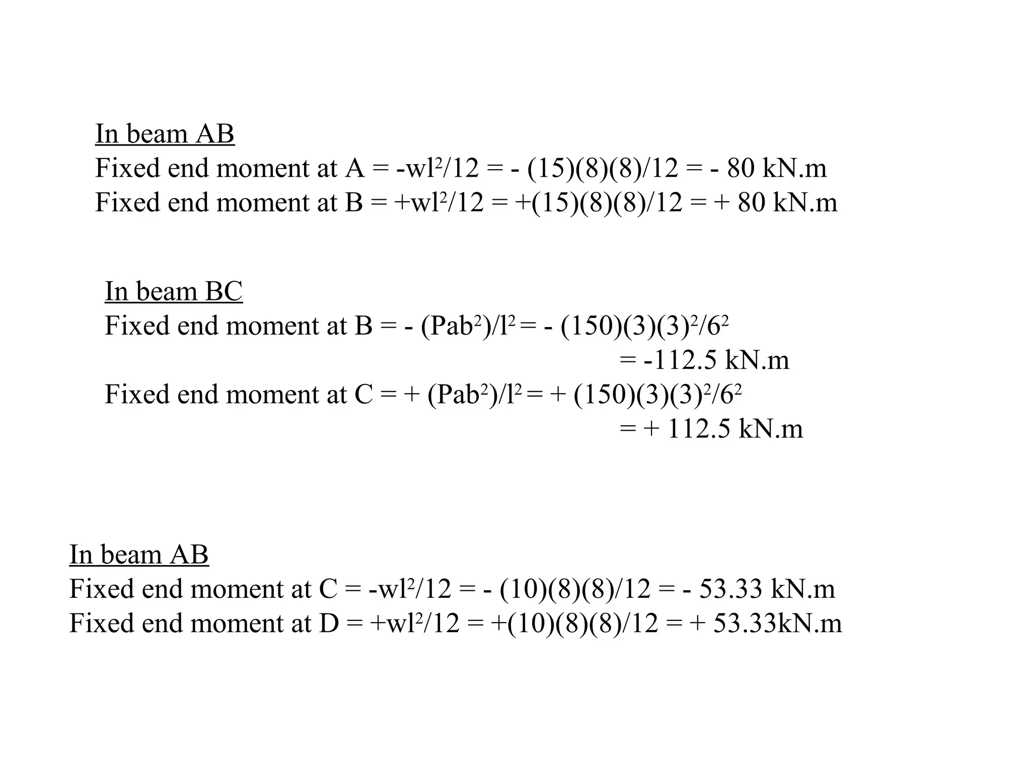
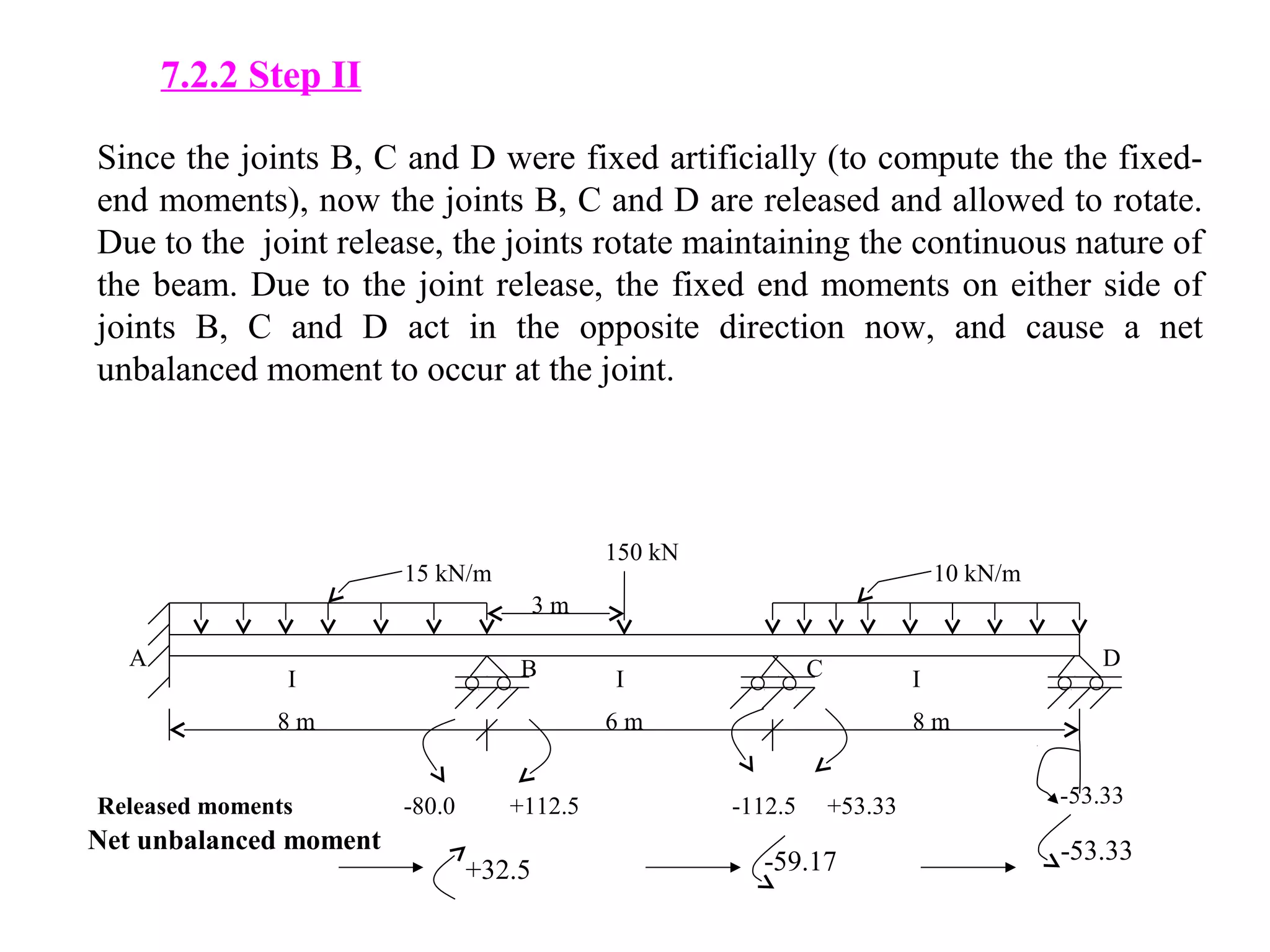
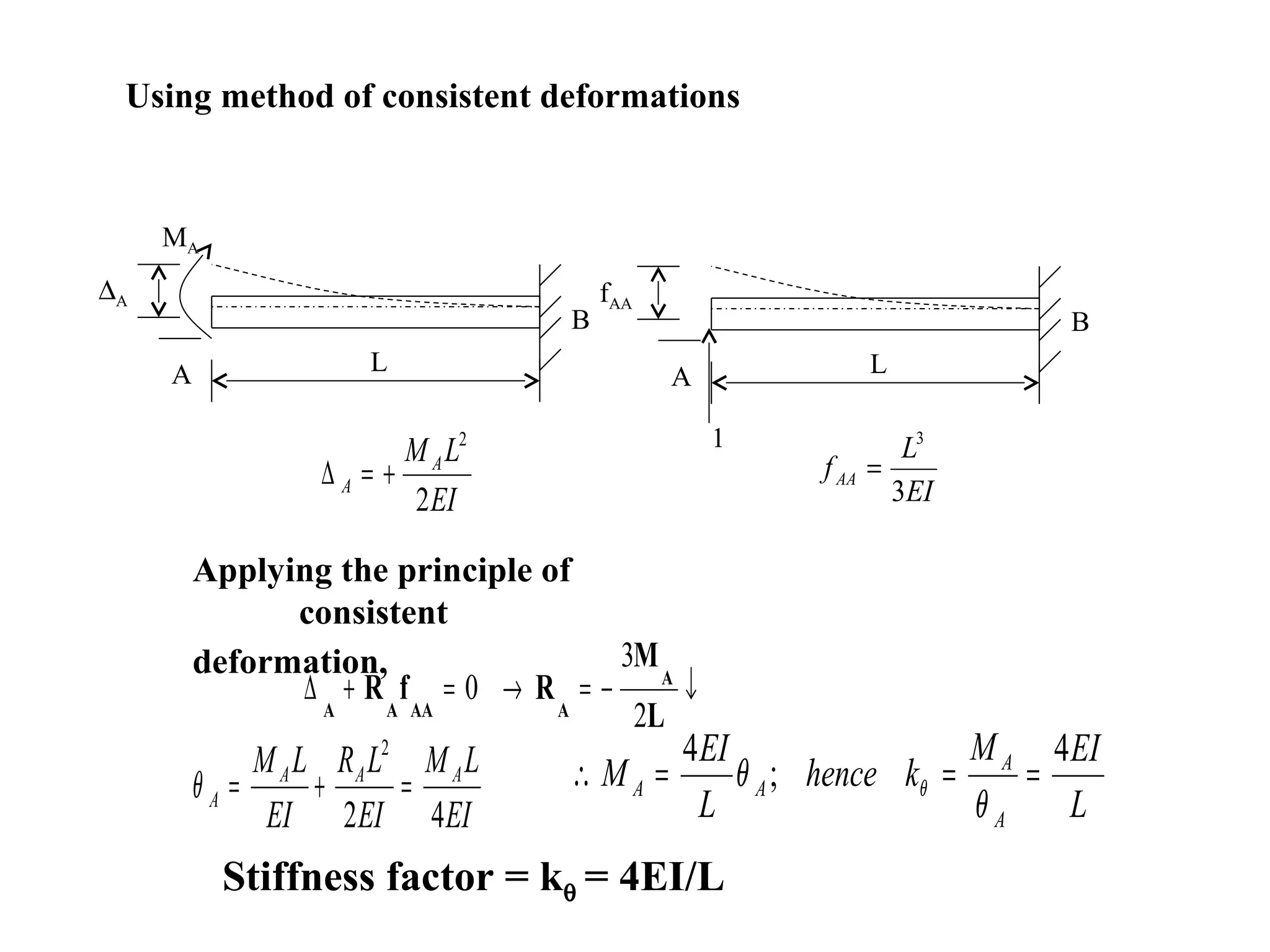
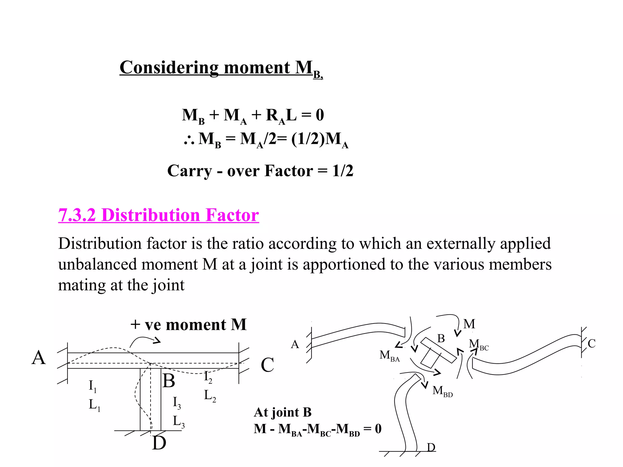
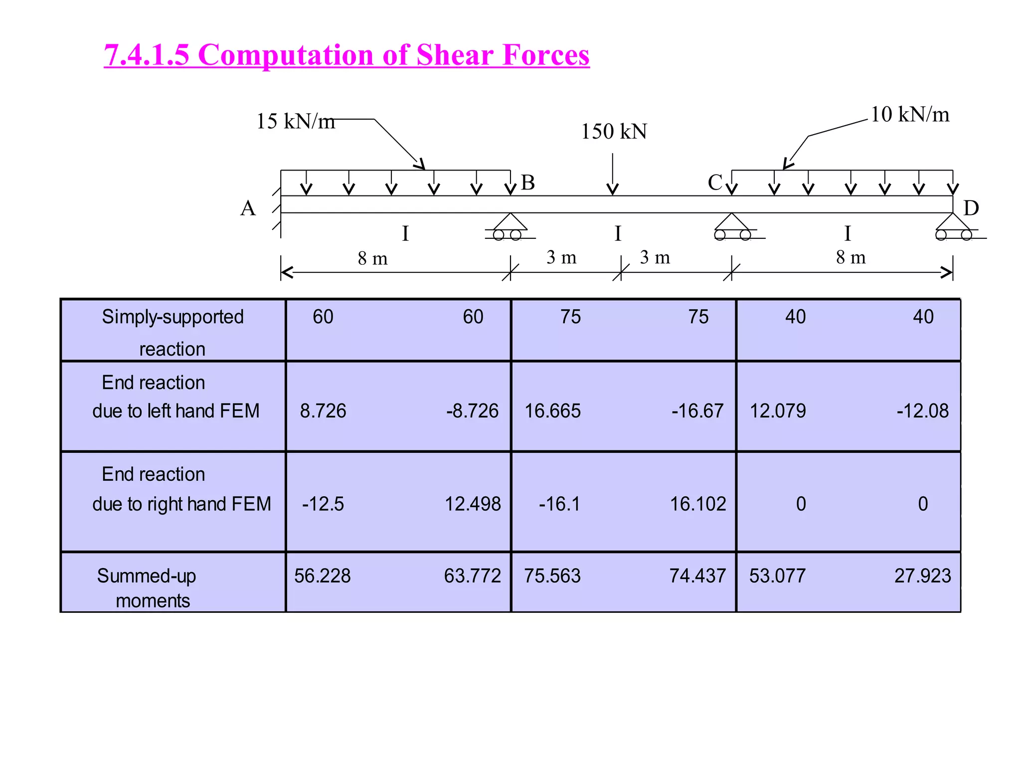
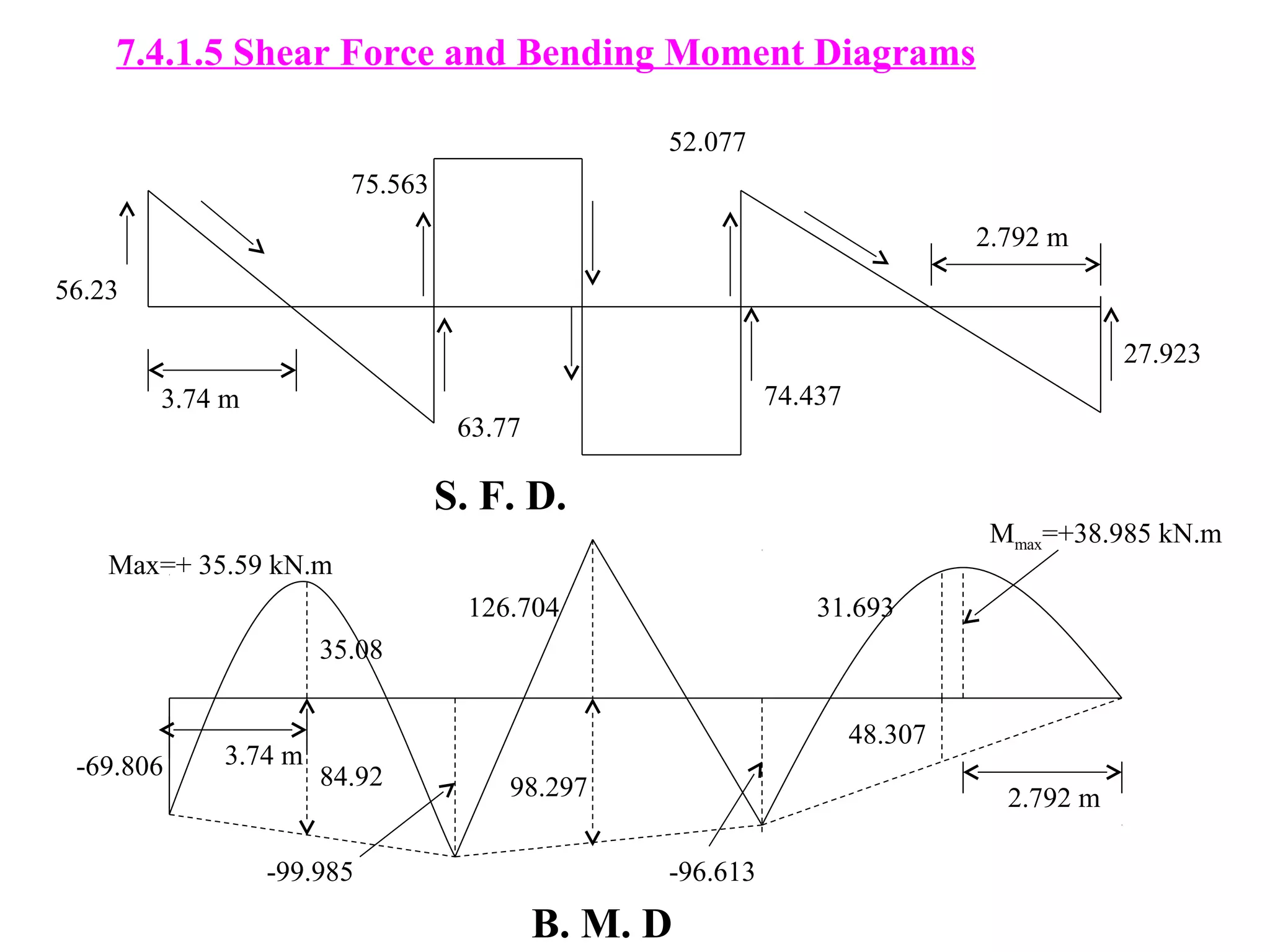
The document discusses the moment distribution method for analyzing statically indeterminate structures. It begins by outlining the basic principles and definitions of the method, including stiffness factors, carry-over factors, and distribution factors. It then provides an example problem, showing the calculation of fixed end moments, establishment of the distribution table through successive approximations, and determination of shear forces and bending moments. Finally, it discusses extensions of the method to structures with non-prismatic members, including using tables to determine necessary values for analysis.

1. Government Engineering College, Bhavnagar.
Civil Engineering Department

2. MOMENT DISTRIBUTION METHOD

3. 7.1 MOMENT DISTRIBUTION METHOD - AN
OVERVIEW
• 7.1 MOMENT DISTRIBUTION METHOD - AN OVERVIEW
• 7.2 INTRODUCTION
• 7.3 STATEMENT OF BASIC PRINCIPLES
• 7.4 SOME BASIC DEFINITIONS
• 7.5 SOLUTION OF PROBLEMS
• 7.6 MOMENT DISTRIBUTION METHOD FOR STRUCTURES
HAVING NONPRISMATIC MEMBERS

4. 7.2 MOMENT DISTRIBUTION METHOD -
INTRODUCTION AND BASIC PRINCIPLES
7.1 Introduction
(Method developed by Prof. Hardy Cross in 1932)
The method solves for the joint moments in continuous beams and
rigid frames by successive approximation.
7.2 Statement of Basic Principles
Consider the continuous beam ABCD, subjected to the given loads,
as shown in Figure below. Assume that only rotation of joints
occur
at B, C and D, and that no support displacements occur at B, C and
D. Due to the applied loads in spans AB, BC and CD, rotations
occur at B, C and D.
15 kN/m 10 kN/m
150 kN
8 m 6 m 8 m
A B C D
I I I
3 m

5. In order to solve the problem in a successively approximating manner,
it can be visualized to be made up of a continued two-stage problems
viz., that of locking and releasing the joints in a continuous sequence.
7.2.1 Step I
The joints B, C and D are locked in position before any load is
applied on the beam ABCD; then given loads are applied on the
beam. Since the joints of beam ABCD are locked in position, beams
AB, BC and CD acts as individual and separate fixed beams,
subjected to the applied loads; these loads develop fixed end
moments.
8 m
-80 kN.m -80 kN.m15 kN/m
A B
6 m
-112.5kN.m 112.5 kN.m
B C 8 m
-53.33 kN.m
10 kN/m
C D
150 kN
53.33 kN.m
3 m

6. In beam AB
Fixed end moment at A = -wl2
/12 = - (15)(8)(8)/12 = - 80 kN.m
Fixed end moment at B = +wl2
/12 = +(15)(8)(8)/12 = + 80 kN.m
In beam BC
Fixed end moment at B = - (Pab2
)/l2
= - (150)(3)(3)2
/62
= -112.5 kN.m
Fixed end moment at C = + (Pab2
)/l2
= + (150)(3)(3)2
/62
= + 112.5 kN.m
In beam AB
Fixed end moment at C = -wl2
/12 = - (10)(8)(8)/12 = - 53.33 kN.m
Fixed end moment at D = +wl2
/12 = +(10)(8)(8)/12 = + 53.33kN.m

7. 7.2.2 Step II
Since the joints B, C and D were fixed artificially (to compute the the fixed-
end moments), now the joints B, C and D are released and allowed to rotate.
Due to the joint release, the joints rotate maintaining the continuous nature of
the beam. Due to the joint release, the fixed end moments on either side of
joints B, C and D act in the opposite direction now, and cause a net
unbalanced moment to occur at the joint.
15 kN/m 10 kN/m
8 m 6 m 8 m
A B C D
I I I
3 m
150 kN
Released moments -80.0 -112.5 +53.33 -53.33+112.5
Net unbalanced moment
+32.5 -59.17 -53.33

8. 7.2.3 Step III
These unbalanced moments act at the joints and modify the joint moments at
B, C and D, according to their relative stiffnesses at the respective joints. The
joint moments are distributed to either side of the joint B, C or D, according
to their relative stiffnesses. These distributed moments also modify the
moments at the opposite side of the beam span, viz., at joint A in span AB, at
joints B and C in span BC and at joints C and D in span CD. This
modification is dependent on the carry-over factor (which is equal to 0.5 in
this case); when this carry over is made, the joints on opposite side are
assumed to be fixed.
7.2.4 Step IV
The carry-over moment becomes the unbalanced moment at the joints
to which they are carried over. Steps 3 and 4 are repeated till the carry-
over or distributed moment becomes small.
7.2.5 Step V
Sum up all the moments at each of the joint to obtain the joint
moments.

9. 7.3 SOME BASIC DEFINITIONS
In order to understand the five steps mentioned in section 7.3, some words
need to be defined and relevant derivations made.
7.3.1 Stiffness and Carry-over Factors
Stiffness = Resistance offered by member to a unit displacement or rotation at a
point, for given support constraint conditions
θA
MA
MB
A BA
RA RB
L
E, I – Member properties
A clockwise moment MA is
applied at A to produce a +ve
bending in beam AB. Find θA
and MB.

10. Using method of consistent deformations
L
∆A
A
MA
B
L
fAA
A
B
1
EI
LM A
A
2
2
+=∆
EI
L
fAA
3
3
=
Applying the principle of
consistent
deformation,
↓−=→=+∆
L
M
RfR A
AAAAA 2
3
0
EI
LM
EI
LR
EI
LM AAA
A
42
2
=+=θ
L
EIM
khence
L
EI
M
A
A
AA
4
;
4
===∴
θ
θ θ
Stiffness factor = kθ = 4EI/L

11. Considering moment MB,
MB + MA + RAL = 0
∴MB = MA/2= (1/2)MA
Carry - over Factor = 1/2
7.3.2 Distribution Factor
Distribution factor is the ratio according to which an externally applied
unbalanced moment M at a joint is apportioned to the various members
mating at the joint
+ ve moment M
A C
B
D
A
D
B C
MBA
MBC
MBD
At joint B
M - MBA-MBC-MBD = 0
I1
L1
I3
L3
I2
L2
M

12. i.e., M = MBA + MBC + MBD
( )
( )
MFDM
K
K
M
MFDM
K
K
M
Similarly
MFDM
K
K
KM
K
M
KKK
M
KKK
L
IE
L
IE
L
IE
BD
BD
BD
BC
BC
BC
BA
BA
BBABA
BDBCBA
B
BBDBCBA
B
).(
).(
).(
444
3
33
2
22
1
11
=








=
=








=
=








==
=
++
=∴
++=












+





+





=
∑
∑
∑
∑
θ
θ
θ
θ

13. 7.3.3 Modified Stiffness Factor
The stiffness factor changes when the far end of the beam is simply-
supported.
θAMA
A B
RA RB
L
As per earlier equations for deformation, given in Mechanics of Solids
text-books.
fixedAB
A
A
AB
A
A
K
L
EI
L
EIM
K
EI
LM
)(
4
3
4
4
33
3
=












===
=
θ
θ

14. 7.4 SOLUTION OF PROBLEMS -
7.4.1 Solve the previously given problem by the moment
distribution method
7.4.1.1: Fixed end moments
mkN
wl
MM
mkN
wl
MM
mkN
wl
MM
DCCD
CBBC
BAAB
.333.53
12
)8)(10(
12
.5.112
8
)6)(150(
8
.80
12
)8)(15(
12
22
22
−=−=−=−=
−=−=−=−=
−=−=−=−=
7.4.1.2 Stiffness Factors (Unmodified Stiffness)
EI
EI
K
EIEI
EI
K
EI
EI
L
EI
KK
EI
EI
L
EI
KK
DC
CD
CBBC
BAAB
5.0
8
4
5.0
8
4
8
4
667.0
6
))(4(4
5.0
8
))(4(4
==
==





=
====
====

15. 7.4.1.3 Distribution Factors
00.1
4284.0
500.0667.0
500.0
5716.0
500.0667.0
667.0
5716.0
667.05.0
667.0
4284.0
667.05.0
5.0
0.0
)(5.0
5.0
==
=
+
=
+
=
=
+
=
+
=
=
+
=
+
=
=
+
=
+
=
=
∞+
=
+
=
DC
DC
DC
CDCB
CD
CD
CDCB
CB
CB
BCBA
BC
BC
BCBA
BA
BA
wallBA
BA
AB
K
K
DF
EIEI
EI
KK
K
DF
EIEI
EI
KK
K
DF
EIEI
EI
KK
K
DF
EIEI
EI
KK
K
DF
stiffnesswall
EI
KK
K
DF

16. Joint A B C D
Member AB BA BC CB CD DC
Distribution Factors 0 0.4284 0.5716 0.5716 0.4284 1
Computed end moments -80 80 -112.5 112.5 -53.33 53.33
Cycle 1
Distribution 13.923 18.577 -33.82 -25.35 -53.33
Carry-over moments 6.962 -16.91 9.289 -26.67 -12.35
Cycle 2
Distribution 7.244 9.662 9.935 7.446 12.35
Carry-over moments 3.622 4.968 4.831 6.175 3.723
Cycle 3
Distribution -2.128 -2.84 -6.129 -4.715 -3.723
Carry-over moments -1.064 -3.146 -1.42 -1.862 -2.358
Cycle 4
Distribution 1.348 1.798 1.876 1.406 2.358
Carry-over moments 0.674 0.938 0.9 1.179 0.703
Cycle 5
Distribution -0.402 -0.536 -1.187 -0.891 -0.703
Summed up -69.81 99.985 -99.99 96.613 -96.61 0
moments
7.4.1.4 Moment Distribution Table

17. 7.4.1.5 Computation of Shear Forces
Simply-supported 60 60 75 75 40 40
reaction
End reaction
due to left hand FEM 8.726 -8.726 16.665 -16.67 12.079 -12.08
End reaction
due to right hand FEM -12.5 12.498 -16.1 16.102 0 0
Summed-up 56.228 63.772 75.563 74.437 53.077 27.923
moments
8 m 3 m 3 m 8 m
I I I
15 kN/m 10 kN/m
150 kN
A
B C
D

18. 7.4.1.5 Shear Force and Bending Moment Diagrams
56.23
3.74 m
75.563
63.77
52.077
74.437
27.923
2.792 m
-69.806
98.297
35.08
126.704
-96.613
31.693
Mmax=+38.985 kN.m
Max=+ 35.59 kN.m
3.74 m
84.92
-99.985
48.307
2.792 m
S. F. D.
B. M. D

19. Simply-supported bending moments at center of span
Mcenter in AB = (15)(8)2
/8 = +120 kN.m
Mcenter in BC = (150)(6)/4 = +225 kN.m
Mcenter in AB = (10)(8)2
/8 = +80 kN.m

20. 7.5 MOMENT DISTRIBUTION METHOD FOR
NONPRISMATIC MEMBER (CHAPTER 12)
The section will discuss moment distribution method to analyze
beams and frames composed of nonprismatic members. First
the procedure to obtain the necessary carry-over factors,
stiffness factors and fixed-end moments will be outlined. Then
the use of values given in design tables will be illustrated.
Finally the analysis of statically indeterminate structures using
the moment distribution method will be outlined

21. 7.5.1 Stiffness and Carry-over Factors
Use moment-area method to find the stiffness and carry-
over factors of the non-prismatic beam.
∆
A
B
PA MB
MA
θA
AABAA KP ∆= )( ( )
AABB
AABA
MCM
KM
=
= θθ
CAB= Carry-over factor of moment MA from A to B

22. A
B
M′A=CBAMB
=CBAKB
M′B(≡KB)MB=CABMA
=CABKA
MA(≡KA)
θA (= 1.0)
MA θB (= 1.0)
A
B
(a) (b)
Use of Betti-Maxwell’s reciprocal theorem requires that the work
done by loads in case (a) acting through displacements in case (b) is
equal to work done by loads in case (b) acting through displacements in
case (a)
( ) ( ) ( ) ( )
BA
BABA
KK
MMMM
BAAB CC
)0.0()0.1()1()0(
=
′+′=+
MB

23. 7.5.2 Tabulated Design Tables
Graphs and tables have been made available to determine fixed-end
moments, stiffness factors and carry-over factors for common
structural shapes used in design. One such source is the Handbook of
Frame constants published by the Portland Cement Association,
Chicago, Illinois, U. S. A. A portion of these tables, is listed here as
Table 1 and 2
Nomenclature of the Tables
aA ab = ratio of length of haunch (at end A and B to the length
of span
b = ratio of the distance (from the concentrated load to end A)
to the length of span
hA, hB= depth of member at ends A and B, respectively
hC = depth of member at minimum section