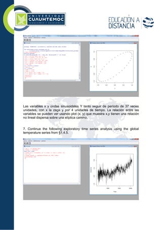
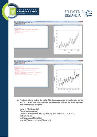
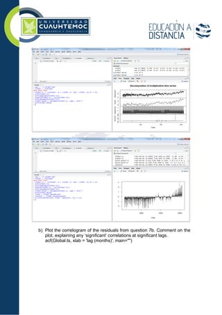
1. The document describes exercises from a statistics modeling course, including instructions to complete exercises 1 and 7 from chapter 3 using provided data files. 2. For exercise 1, the student is asked to describe the association and calculate the cross-correlation between time series variables x and y as the time lag k is varied. For exercise 7, the student continues a time series analysis of global temperature data, including plotting, decomposing, and fitting an appropriate Holt-Winters model to the data. 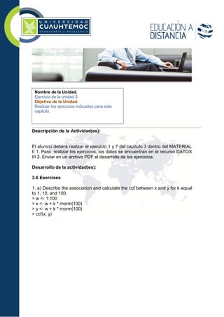3. The student provides their work and results for the exercises, including descriptions of relationships between variables, plots, model fitting, and forecasts for 2005-2010 using the fitted Holt-Winters model. They discuss the validity

1. UNIVERSIDAD CUAUHTÉMOC
PLANTEL AGUASCALIENTES
EDUCACIÓN A DISTANCIA
Maestría en Ciencia de los Datos y
Procesamiento de Datos Masivos
(Big-Data)
Segundo Cuatrimestre
Sergio Andrés Fonseca Chitiva
MODELOS ESTADÍSTICOS DINÁMICOS
Nombre del profesor
Jonás Velasco Alvares
Fecha de entrega
Noviembre 01 2015
“EXCELENTES PROFESIONISTAS, MEJORES SERES HUMANOS”

2. Descripción de la Actividad(es):
El alumno deberá realizar el ejercicio 1 y 7 del capítulo 3 dentro del MATERIAL
II 1. Para realizar los ejercicios, los datos se encuentran en el recurso DATOS
III 2. Enviar en un archivo PDF el desarrollo de los ejercicios.
Desarrollo de la actividad(es):
3.6 Exercises
1. a) Describe the association and calculate the ccf between x and y for k equal
to 1, 10, and 100.
> w <- 1:100
> x <- w + k * rnorm(100)
> y <- w + k * rnorm(100)
> ccf(x, y)
Nombre de la Unidad.
Ejercicio de la unidad 3
Objetivo de la Unidad.
Realizar los ejercicios indicados para este
capitulo.

3. Respecto a x,y están relacionadas de una forma lineal puesto que respeto al
tiempo esta sustrayendo
el t, donde la variable de correlación disminuye a medida que aumenta la
variable k
b) Describe the association between x and y, and calculate the ccf.
> Time <- 1:370
> x <- sin(2 * pi * Time / 37)
> y <- sin(2 * pi * (Time + 4) / 37)
Investigate the effect of adding independent random variation to x
and y.

4. Las variables x y ondas sinusoidales Y tanto seguir de período de 37 veces
unidades, con x la zaga y por 4 unidades de tiempo. La relación entre las
variables se pueden ver usando plot (x, y) que muestra x,y tienen una relación
no lineal dispersa sobre una elíptica camino.
7. Continue the following exploratory time series analysis using the global
temperature series from §1.4.5.

5. a) Produce a time plot of the data. Plot the aggregated annual mean series
and a boxplot that summarises the observed values for each season,
and comment on the plots.
www <- "C:/global.dat"
Global <- scan(www)
Global.ts <- ts(Global, st = c(1856, 1), end = c(2005, 12),fr = 12)
plot(Global.ts)
plot(aggregate(Global.ts))
boxplot(Global.ts ~ cycle(Global.ts))

6. www <- "C:/global.dat"

7. b) Decompose the series into the components trend, seasonal effect, and
residuals, and plot the decomposed series. Produce a plot of the trend with a
superimposed seasonal effect.
plot(decompose(Global.ts))
Global.decom <- decompose(Global.ts, type = "mult")
plot(Global.decom)
Trend <- Global.decom$trend
Seasonal <- Global.decom$seasonal
ts.plot(cbind(Trend, Trend * Seasonal), lty = 1:2)

8. b) Plot the correlogram of the residuals from question 7b. Comment on the
plot, explaining any ‘significant’ correlations at significant lags.
acf(Global.ts, xlab = 'lag (months)', main="")

9. c) Fit an appropriate Holt-Winters model to the monthly data. Explain why
you chose that particular Holt-Winters model, and give the parameter
estimates.
www <- "C:/global.dat"
Global.dat <- read.table(www, header = T); attach(Global.dat)
Global.ts <- ts(Global, st = c(1856, 1), end = c(2005, 12),fr = 12)
plot(Global.ts, xlab = "Time / months", ylab = "Complaints")
> Comp.hw1 <- HoltWinters(Global.ts, beta = 0, gamma = 0) ; Comp.hw1
Holt-Winters exponential smoothing with trend and additive seasonal component.

10. Call:
HoltWinters(x = Global.ts, beta = 0, gamma = 0)
Smoothing parameters:
alpha: 0.2739402
beta : 0
gamma: 0
Coefficients:
[,1]
a 0.455717898
b -0.011593386
s1 0.005628472
s2 0.301878472
s3 -0.067454861
s4 -0.217163194
s5 -0.141163194
s6 0.117961806
s7 0.146878472
s8 0.147295139
s9 -0.016538194
s10 -0.046079861
s11 -0.270329861
s12 0.039086806
>
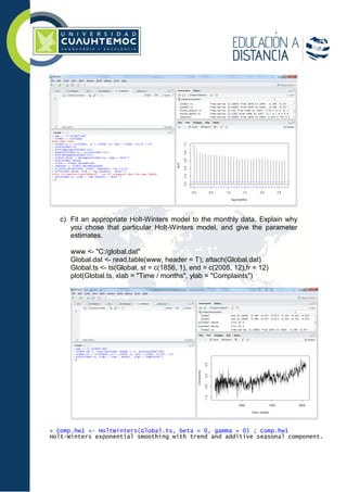
d) Using the fitted model, forecast values for the years 2005–2010. Add
these forecasts to a time plot of the original series. Under what
circumstances would these forecasts be valid? What comments of
caution would you make to an economist or politician who wanted to use
these forecasts to make statements about the potential impact of global
warming on the world economy?

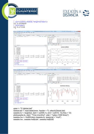
11. > sweetw.hw ; sweetw.hw$coef ; sweetw.hw$SSE
Holt-Winters exponential smoothing with trend and multiplicative seasonal compone
nt.
Call:
HoltWinters(x = sweetw.ts, seasonal = "mult")
Smoothing parameters:
alpha: 0.1318678
beta : 0.01806184
gamma: 0.2098766
Coefficients:
[,1]
a -0.454634140
b -0.004121177
s1 0.905377892
s2 0.604204844
s3 0.920640265
s4 0.992255863
s5 0.938399013
s6 0.529044547
s7 0.536223475
s8 0.492175735
s9 0.836452811
s10 0.846716956
s11 1.389375941
s12 0.876335635
a b s1 s2 s3 s4
-0.454634140 -0.004121177 0.905377892 0.604204844 0.920640265 0.992255863
s5 s6 s7 s8 s9 s10
0.938399013 0.529044547 0.536223475 0.492175735 0.836452811 0.846716956
s11 s12
1.389375941 0.876335635
[1] 5.064764
>

12. www <- "C:/global.dat"
Global.dat <- read.table(www, header = T); attach(Global.dat)
sweetw.ts <- ts(global, start = c(2005,1), end = c(2010, 12),freq = 12)
plot(sweetw.ts, xlab= "Time (months)", ylab = "sales (1000 litres)")
sweetw.hw <- HoltWinters (sweetw.ts, seasonal = "mult")
sweetw.hw ; sweetw.hw$coef ; sweetw.hw$SSE

13. sqrt(sweetw.hw$SSE/length(Global))
sd(Global)
plot (sweetw.hw$fitted)
plot (sweetw.hw)