![Slide 3 www.edureka.co/advanced-predictive-modelling-in-r
a <- ts(1:20, frequency = 12, start = c(2011, 3))
print(a)
## Jan Feb Mar Apr May Jun Jul Aug Sep Oct Nov Dec
## 2011 1 2 3 4 5 6 7 8 9 10
## 2012 11 12 13 14 15 16 17 18 19 20
str(a)
## Time-Series [1:20] from 2011 to 2013: 1 2 3 4 5 6 7 8 9 10 ...
attributes(a)
## $tsp
## [1] 2011.167 2012.750 12.000
##
## $class
## [1] "ts"
Creating a Simple TimeSeries](https://image.slidesharecdn.com/apmrwebinarppt-150316034341-conversion-gate01/85/Webinar-The-Whys-and-Hows-of-Predictive-Modelling-3-320.jpg)
![Slide 4 www.edureka.co/advanced-predictive-modelling-in-r
str(AirPassengers)
## Time-Series [1:144] from 1949 to 1961: 112 118 132 129 121 135 148 148
136 119 ...
summary(AirPassengers)
## Min. 1st Qu. Median Mean 3rd Qu. Max.
## 104.0 180.0 265.5 280.3 360.5 622.0
AirPassengers Case](https://image.slidesharecdn.com/apmrwebinarppt-150316034341-conversion-gate01/85/Webinar-The-Whys-and-Hows-of-Predictive-Modelling-4-320.jpg)
![Slide 6 www.edureka.co/advanced-predictive-modelling-in-r
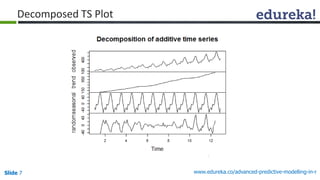
Decomposing the TS
f <- decompose(apts)
> names(f) [1] "x" "seasonal" "trend" "random" "figure" "type"
plot(f$figure, type = "b") # seasonal figures](https://image.slidesharecdn.com/apmrwebinarppt-150316034341-conversion-gate01/85/Webinar-The-Whys-and-Hows-of-Predictive-Modelling-6-320.jpg)
![Slide 16 www.edureka.co/advanced-predictive-modelling-in-r
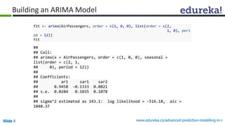
Fitting a Model
fit <- Arima(euretail, order=c(0,1,1), seasonal=c(0,1,1))
fit
## Series: euretail
## ARIMA(0,1,1)(0,1,1)[4]
##
## Coefficients:
## ma1 sma1
## 0.2901 -0.6909
## s.e. 0.1118 0.1197
##
## sigma^2 estimated as 0.1812: log likelihood=-34.68
## AIC=75.36 AICc=75.79 BIC=81.59](https://image.slidesharecdn.com/apmrwebinarppt-150316034341-conversion-gate01/85/Webinar-The-Whys-and-Hows-of-Predictive-Modelling-16-320.jpg)
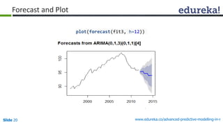
![Slide 18 www.edureka.co/advanced-predictive-modelling-in-r
Lets Tweak the Model
### Lets tweak the Model and try
fit3 <- Arima(euretail, order=c(0,1,3), seasonal=c(0,1,1))
fit3
## Series: euretail
## ARIMA(0,1,3)(0,1,1)[4]
##
## Coefficients:
## ma1 ma2 ma3 sma1
## 0.2625 0.3697 0.4194 -0.6615
## s.e. 0.1239 0.1260 0.1296 0.1555
##
## sigma^2 estimated as 0.1451: log likelihood=-28.7
## AIC=67.4 AICc=68.53 BIC=77.78](https://image.slidesharecdn.com/apmrwebinarppt-150316034341-conversion-gate01/85/Webinar-The-Whys-and-Hows-of-Predictive-Modelling-18-320.jpg)
![Slide 21 www.edureka.co/advanced-predictive-modelling-in-r
Can R Do It Automatically For Us??
auto.arima(euretail)
## Series: euretail
## ARIMA(1,1,1)(0,1,1)[4]
##
## Coefficients:
## ar1 ma1 sma1
## 0.8828 -0.5208 -0.9704
## s.e. 0.1424 0.1755 0.6792
##
## sigma^2 estimated as 0.1411: log likelihood=-30.19
## AIC=68.37 AICc=69.11 BIC=76.68
auto.arima(euretail, stepwise=FALSE, approximation=FALSE)
## Series: euretail
## ARIMA(0,1,3)(0,1,1)[4]
##
## Coefficients:
## ma1 ma2 ma3 sma1
## 0.2625 0.3697 0.4194 -0.6615
## s.e. 0.1239 0.1260 0.1296 0.1555
##
## sigma^2 estimated as 0.1451: log likelihood=-28.7
## AIC=67.4 AICc=68.53 BIC=77.78](https://image.slidesharecdn.com/apmrwebinarppt-150316034341-conversion-gate01/85/Webinar-The-Whys-and-Hows-of-Predictive-Modelling-21-320.jpg)
![Slide 22 www.edureka.co/advanced-predictive-modelling-in-r
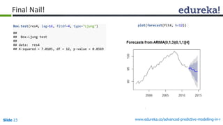
Final Model
fit4<-auto.arima(euretail, stepwise=FALSE, approximation=FALSE)
fit4
## Series: euretail
## ARIMA(0,1,3)(0,1,1)[4]
##
## Coefficients:
## ma1 ma2 ma3 sma1
## 0.2625 0.3697 0.4194 -0.6615
## s.e. 0.1239 0.1260 0.1296 0.1555
##
## sigma^2 estimated as 0.1451: log likelihood=-28.7
## AIC=67.4 AICc=68.53 BIC=77.78
res4 <- residuals(fit4)
tsdisplay(res4)](https://image.slidesharecdn.com/apmrwebinarppt-150316034341-conversion-gate01/85/Webinar-The-Whys-and-Hows-of-Predictive-Modelling-22-320.jpg)


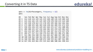
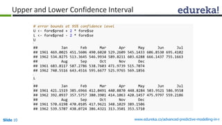
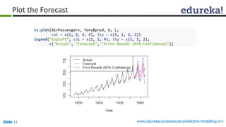
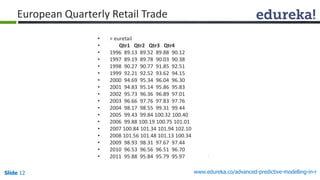
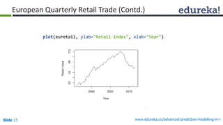
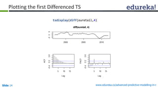
The document provides an overview of advanced predictive modeling techniques using R, including time-series analysis, ARIMA model building, and forecasting methods. It features examples like air passenger data and European retail trade data, showing how to analyze and plot these datasets. Key objectives include understanding predictive modeling concepts, handling real-life datasets, and applying various forecasting techniques.


![ARIMA Models - [Lab 3]](https://cdn.slidesharecdn.com/ss_thumbnails/ydqcxn5vtqizjoun2as1-signature-e1de5ad681d661531c2467ca0d3e475440809ccfdbcb78c5369a1bb749945888-poli-141230090527-conversion-gate01-thumbnail.jpg?width=640&height=640&fit=bounds)