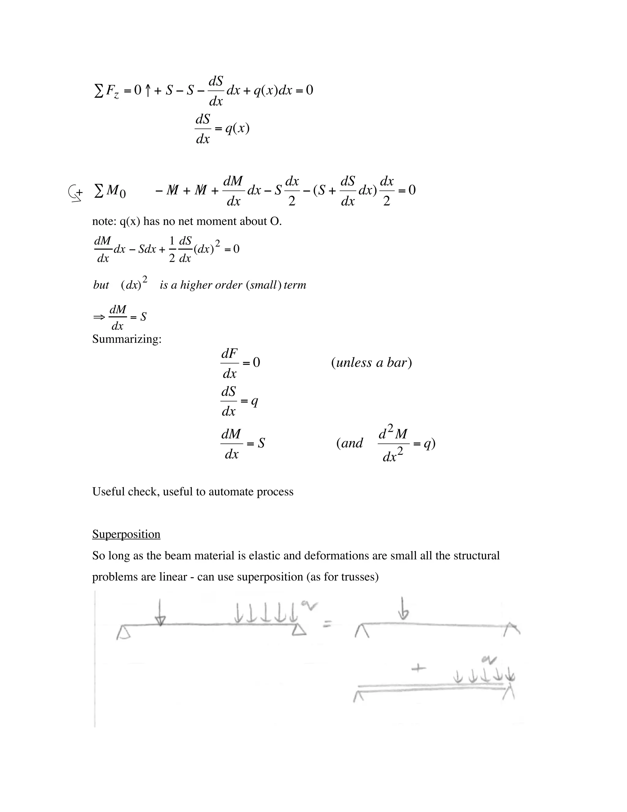
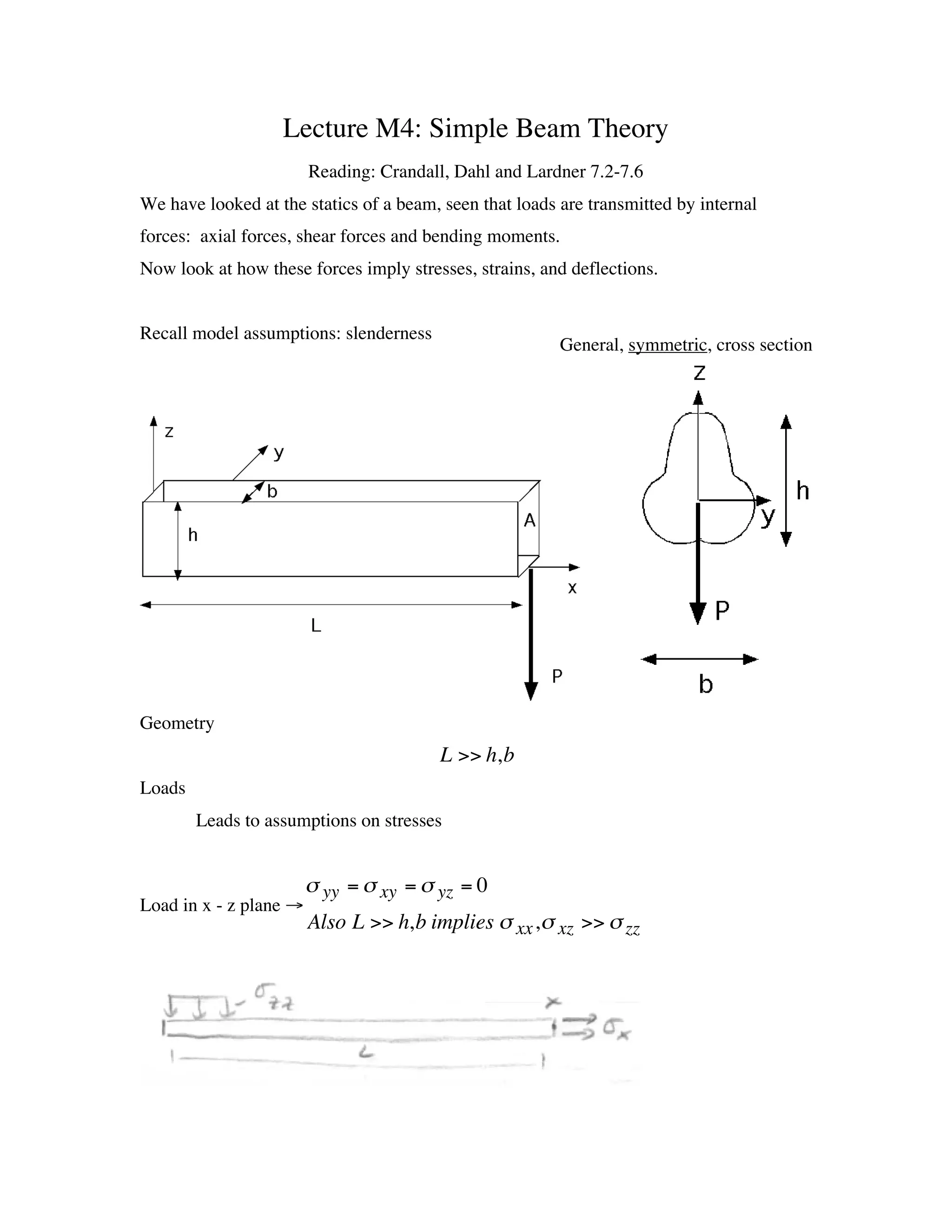
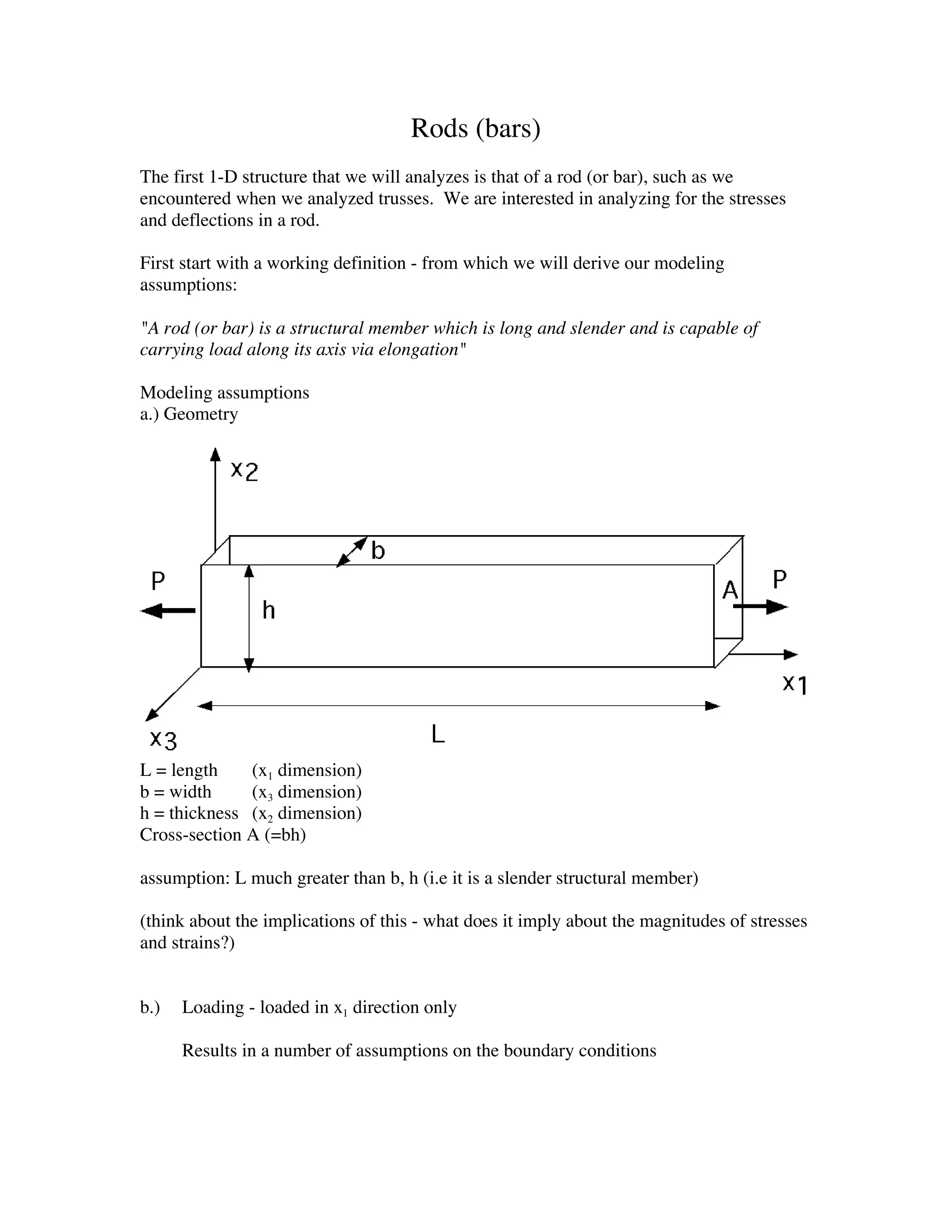
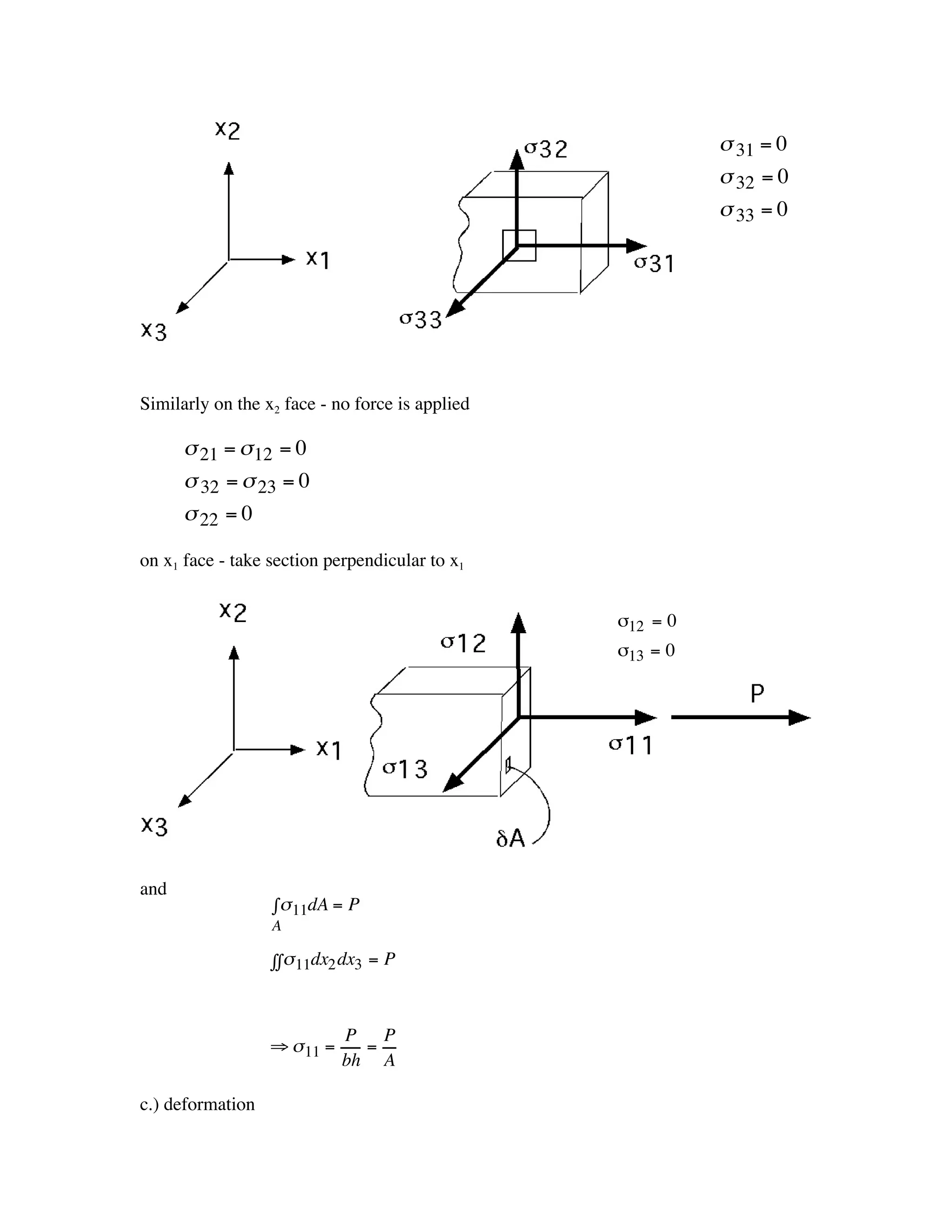
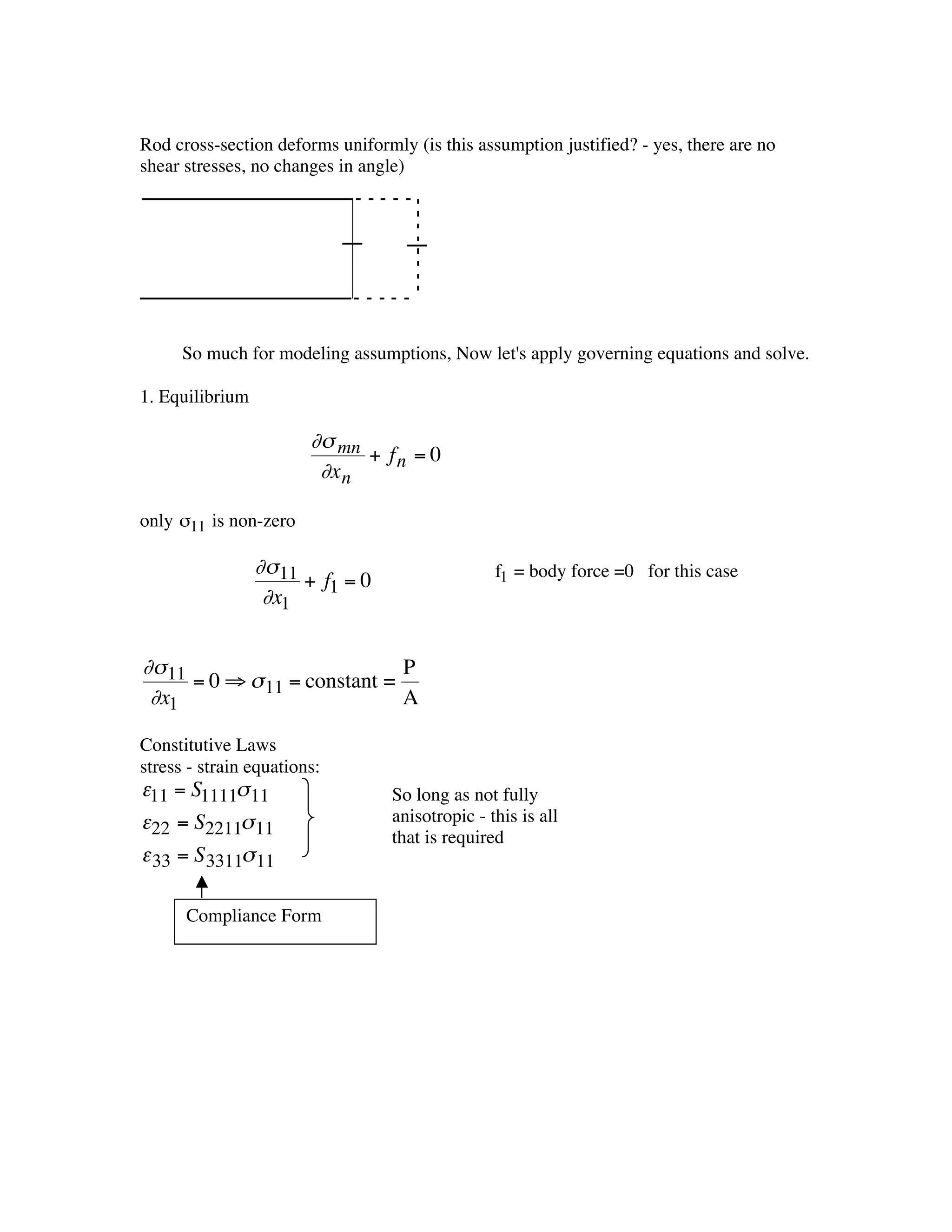
This document provides an overview of analyzing slender structural members like rods, beams, shafts and columns. It outlines the basic logical steps to follow: 1) Make general and problem-specific modeling assumptions for geometry, loading, deformation and boundary conditions. 2) Apply the appropriate governing equations from elasticity. 3) Use an exact analytical or approximate numerical solution method. It then provides more details on modeling assumptions and solving for stresses and deflections in rods under axial loading as an example.

1. Lecture M1 Slender (one dimensional) Structures
Reading: Crandall, Dahl and Lardner 3.1, 7.2
This semester we are going to utilize the principles we learnt last semester (i.e the 3 great
principles and their embodiment in the 15 continuum equations of elasticity) in order to
be able to analyze simple structural members. These members are: Rods, Beams, Shafts
and Columns. The key feature of all these structures is that one dimension is longer than
the others (i.e. they are one dimensional).
Understanding how these structural members carry loads and undergo deformations will
also take us a step nearer being able to design and analyze structures typically found in
aerospace applications. Slender wings behave much like beams, rockets for launch
vehicles carry axial compressive loads like columns, gas turbine engines and helicopter
rotors have shafts to transmit the torque between the components andspace structures
consist of trusses containing rods. You should also be aware that real aerospace
structures are more complicated than these simple idealizations, but at the same time, a
good understanding of these idealizations is an important starting point for further
progress.
There is a basic logical set of steps that we will follow for each in turn.
1) We will make general modeling assumptions for the particular class of structural
member
In general these will be on:
a) Geometry
b) Loading/Stress State
c) Deformation/Strain State
2) We will make problem-specific modeling assumptions on the boundary conditions that
apply (idealized supports, such as pins, clamps, rollers that we encountered with truss
structures last semester)
a.) On stresses Applied at specified
b.) On displacements locations in structure
3) We will apply an appropriate solution method:
a) Exact/analytical (Unified, 16.20)
b Approximate (often numerical) (16.21). Such as energy methods (finite
elements, finite difference - use computers)
Let us see how this works:

2. Rods (bars)
The first 1-D structure that we will analyzes is that of a rod (or bar), such as we
encountered when we analyzed trusses. We are interested in analyzing for the stresses
and deflections in a rod.
First start with a working definition - from which we will derive our modeling
assumptions:
"A rod (or bar) is a structural member which is long and slender and is capable of
carrying load along its axis via elongation"
Modeling assumptions
a.) Geometry
L = length (x1 dimension)
b = width (x3 dimension)
h = thickness (x2 dimension)
Cross-section A (=bh)
assumption: L much greater than b, h (i.e it is a slender structural member)
(think about the implications of this - what does it imply about the magnitudes of stresses
and strains?)
b.) Loading - loaded in x1 direction only
Results in a number of assumptions on the boundary conditions

3. s 31 = 0
s 32 = 0
s 33 = 0
†
Similarly on the x2 face - no force is applied
s 21 = s 12 = 0
s 32 = s 23 = 0
s 22 = 0
on x1 face - take section perpendicular to x1
†
s12 = 0
s13 = 0
and
Ú s 11dA = P
A
ÚÚ s 11dx2 dx3 = P
P P
fi s 11 = =
bh A
c.) deformation

4. Rod cross-section deforms uniformly (is this assumption justified? - yes, there are no
shear stresses, no changes in angle)
So much for modeling assumptions, Now let's apply governing equations and solve.
1. Equilibrium
∂s mn
+ fn = 0
∂x n
only s11 is non-zero
† ∂s 11 f1 = body force =0 for this case
+ f1 = 0
∂x1
∂s 11 P
= 0 fi s 11 = constant =
†
∂x1 A
Constitutive Laws
stress - strain equations:
† e11 = S1111s 11 So long as not fully
e22 = S2211s 11 anisotropic - this is all
that is required
e 33 = S 3311s 11
Compliance Form
†

5. 1 1
S1111 = e11 = s 11
Ex E
n xy -n
S2211 = - For isotropic material gives: e22 = s 11
Ex E
n -n
S 3311 = - xz e 33 = s 11
E
Ex
Now apply strain – displacement relations:
†
†
1 Ê∂u ∂u ˆ
e mn = Á m + n ˜
2 Ë ∂xn ∂x m ¯
∂u ∂u ∂u
e11 = 1 , e22 = 2 , e 33 = 3
∂x1 ∂x2 ∂x 3
† Hence (for isotropic material):
s 11 ∂u1
=
E ∂x1
P ∂u1
fi =
AE ∂x1
integration gives:
Px1
u1 = + g(x2 , x 3 )
† AE1
Apply B. C. u1 = 0 @ x1 = 0 fi g(x2 , x 3 ) = 0
†
i.e. uniaxial extension only, fixed at root
† †

6. Px1
fi u1 = .
AE
-nP
similarly u2 = x2
AE
†
-nP
u3 = x3
AE
†
1 Ê ∂u1 ∂u2 ˆ
check: e12 = Á + ˜=0 ÷
2 Ë∂x2 ∂x1 ¯
†
Assessment of assumptions
† (Closer inspection reveals that our solutions are not exact.)
1) Cross section changes shape slightly. A is not a constant.
If we solved the equations of elasticity simultaneously, we would account for this.
Solving them sequentially is ok so long as deformations are small. (dA is second
order.)
2) At attachment point boundary conditions are different from those elsewhere on
the rod.
u1 = 0, u2 = 0, u3 = 0
(Remember recitation example
last term – materials axially
loaded in a rigid container. Also
† problem set question about thin
adhesive joint.)

7. We deal with this by invoking St. Venant's principle:
"Remote from the boundary conditions internal stresses and deformations will be
insensitive to the exact form of the boundary condition."
And the boundary condition can be replaced by a statically equivalent condition
(equipollent) without loss of accuracy.
How far is remote?
This is the importance of the "long slender" wording of the rod definition.
This should have been all fairly obvious. Next time we will start an equivalent process
for beams - which will require a little more thought.

8. M2 Statics of Beams
Reading: Crandall, Dahl and Lardner, 3.2-3.5, 3.6, 3.8
A beam is a structural member which is long and slender and is capable of carrying
bending loads. I.e loads applied transverse to its long axis.
Obvious examples of aerospace interest are wings and other aerodynamic surfaces. Lift
and weight act in a transverse direction to a long slender axis of the wing (think of glider
wings as our prototype beam). Note, even a glider wing is not a pure beam – it will have
to carry torsional loads (aerodynamic moments).
1.) Modeling assumptions
a.) Geometry, slender member, L>>b, h
At this stage, will assume arbitrary, symmetric cross-sections, i.e.:

9. b.) Loading
• Similar to rod (traction free surfaces) but applied loads can be in the z
direction
c.) Deformation
• We will talk about this later
Distributed load
2.) Boundary conditions
As for rod, trusses
Pinned, simply supported Cantilever
Draw FBD, apply equilibrium to determine reactions.
3.) Governing equations
• Equations of elasticity
4.) Solution Method
• Exact (exactly solve governing differential equations)
• Approximate (use numerical solution)
But first need to look at how beams transmit load.
Internal Forces
Apply methods of sections to beam (also change coordinate system – to x, y, z –
consistent with CDL). Method exactly as for trusses. Cut structure at location where we
wish to find internal forces, apply equilibrium, obtain forces. In the case of a beam, the
structure is continuous, rather than consisting of discrete bars, so we will find that the
internal forces (and moments) are, in general, a continuous function of position.

10. Internal forces
Opposite
directions on two
faces - equilibrium

11. (Note Crandall Dahl and Lardner use V = -S)
where M = Bending movement Beam
S = Shear force Bending "beam bar"
F = Axial force bar, rod
Also drawn as
Example of calculating shear force and bending moment distribution along a beam.
Example 1. Cantilever beam.

12. Free Body Diagram (note moment reaction at root)
Equilibrium: H A = 0, VA = P, M A = -PL
Take cut at point X ,distance x from left hand end (root). 0< x < L. Replace
the effect of the (discarded) right hand side of beam by an equivalent set of forces and
moments (M, S, F) which vary as a function of position, x.
†
Apply equilibrium
+
 Fx = 0 Æ F(x) = 0
 Fz = 0 ↑ + P - S(x) = 0 S(x) = P
ÂMX =0 + Pl + M (x) - Px = 0 M (x) = -P(l - x)
†

13. Draw "sketches" - bending moment, shear force, loading diagrams
Axial Force diagram (zero everywhere in this case)
Shear Force Diagram
Bending moment diagram:

14. NOTE: At boundaries values go to reactions (moment at root, applied load at tip).
These representations are useful because they provide us with a visual indication of
where the internal forces on the beam are highest, which will play a role in determining
where failure might occur and how we should design the internal structure of the beam
(put more material where the forces are higher).
Lecture M3 Shear Forces and Bending Moments in Beams
continued: Example 2
Simply supported beam:
Free body diagram:
take cut at 0< x< L/2

15. Equilibrium ÆF(x) = 0
P P
↑ - S(x) = 0 fi S(x) =
2 2 0<x<L
P Px
M x = 0 + fi - x + M (x) = 0 fi M (x) =
2 2
L †
take cut at <x<L
2
†
†

16. Apply equilibrium (moments about X):
P P
 ↑ F+ = 0 : - P - S(x) = 0 fi S(x) = -
2 2
P Ê Lˆ
ÂM =0: - x + PÁ x - ˜ + M (x) = 0
2 Ë 2¯
P
M (x) = - (x - L)
2
† P
= (L - x)
2
Draw Diagrams
†

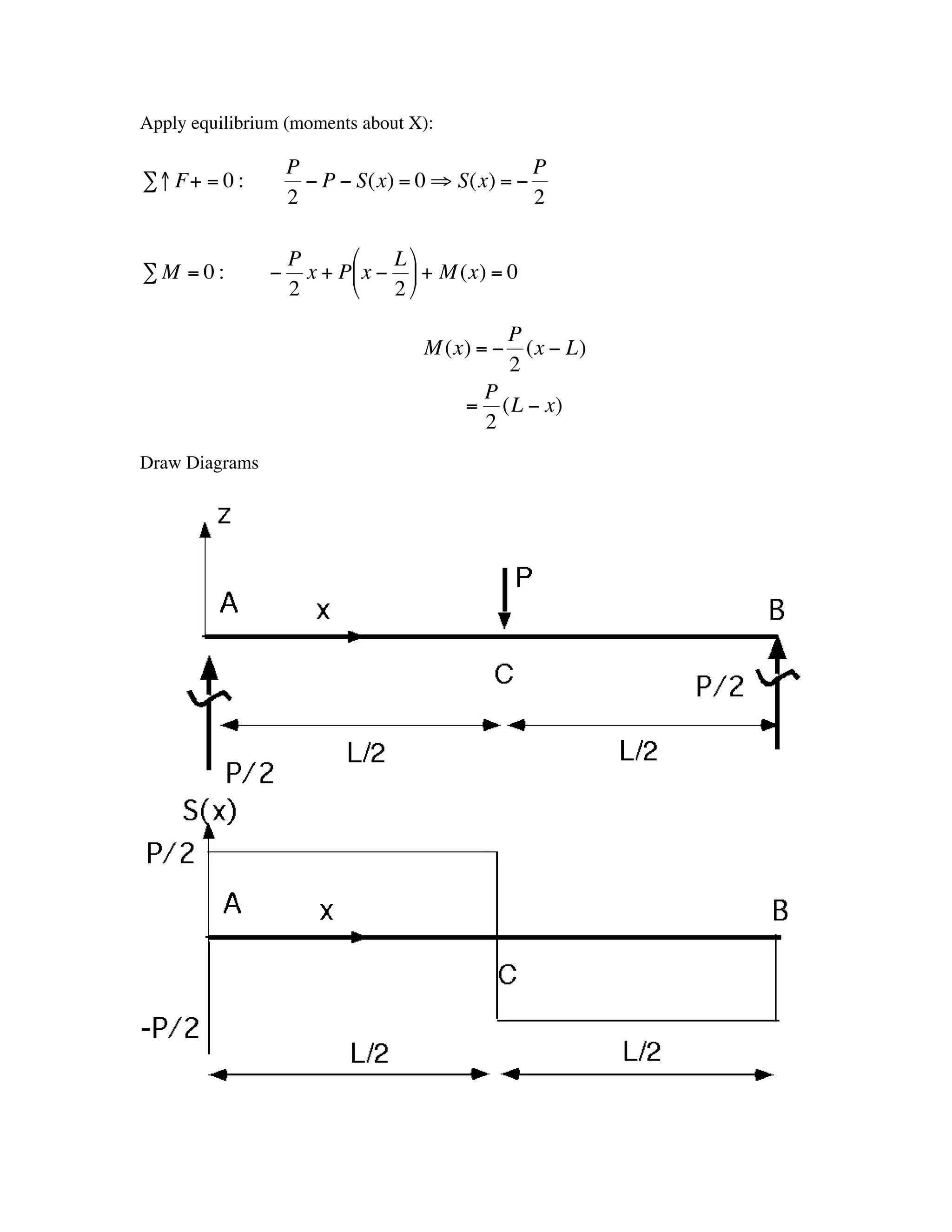
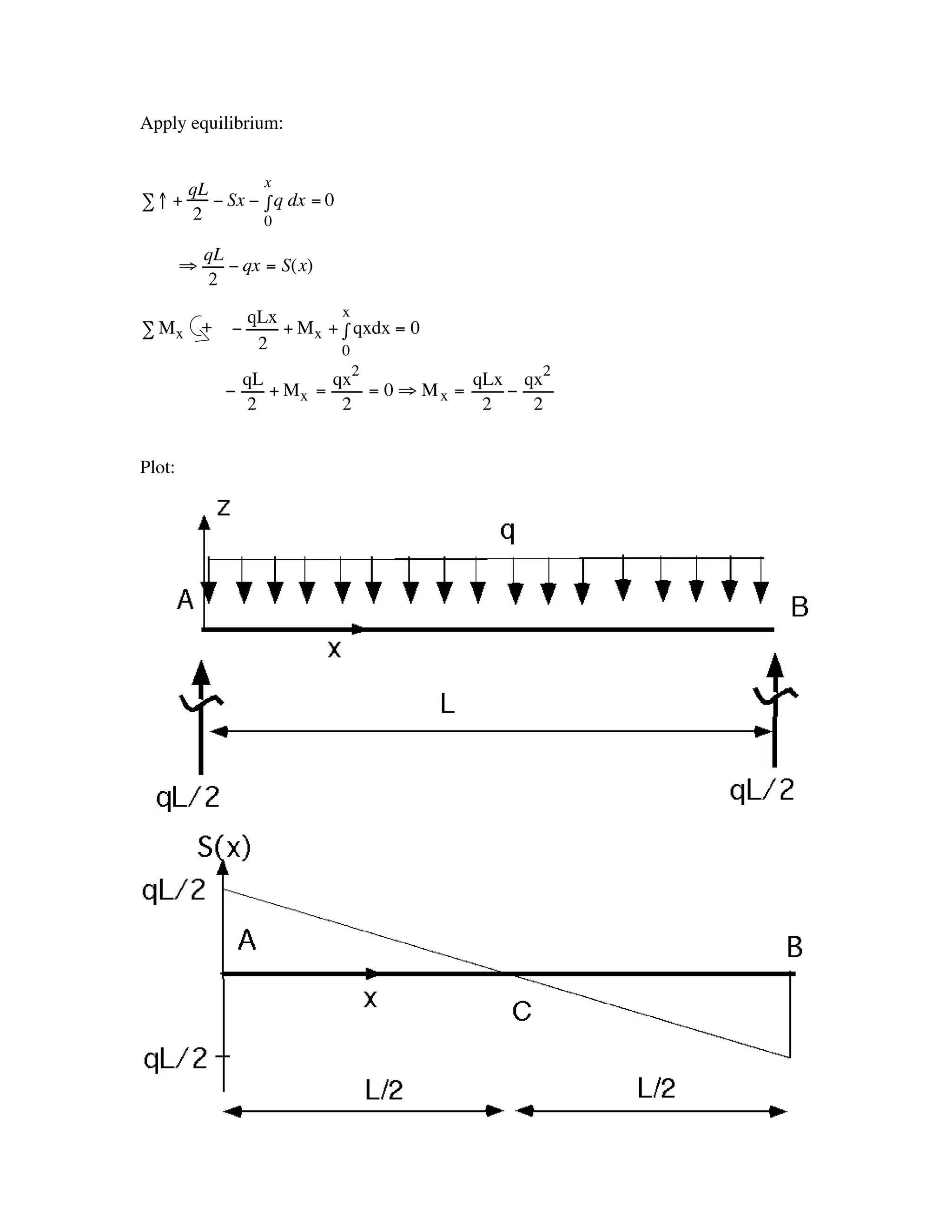
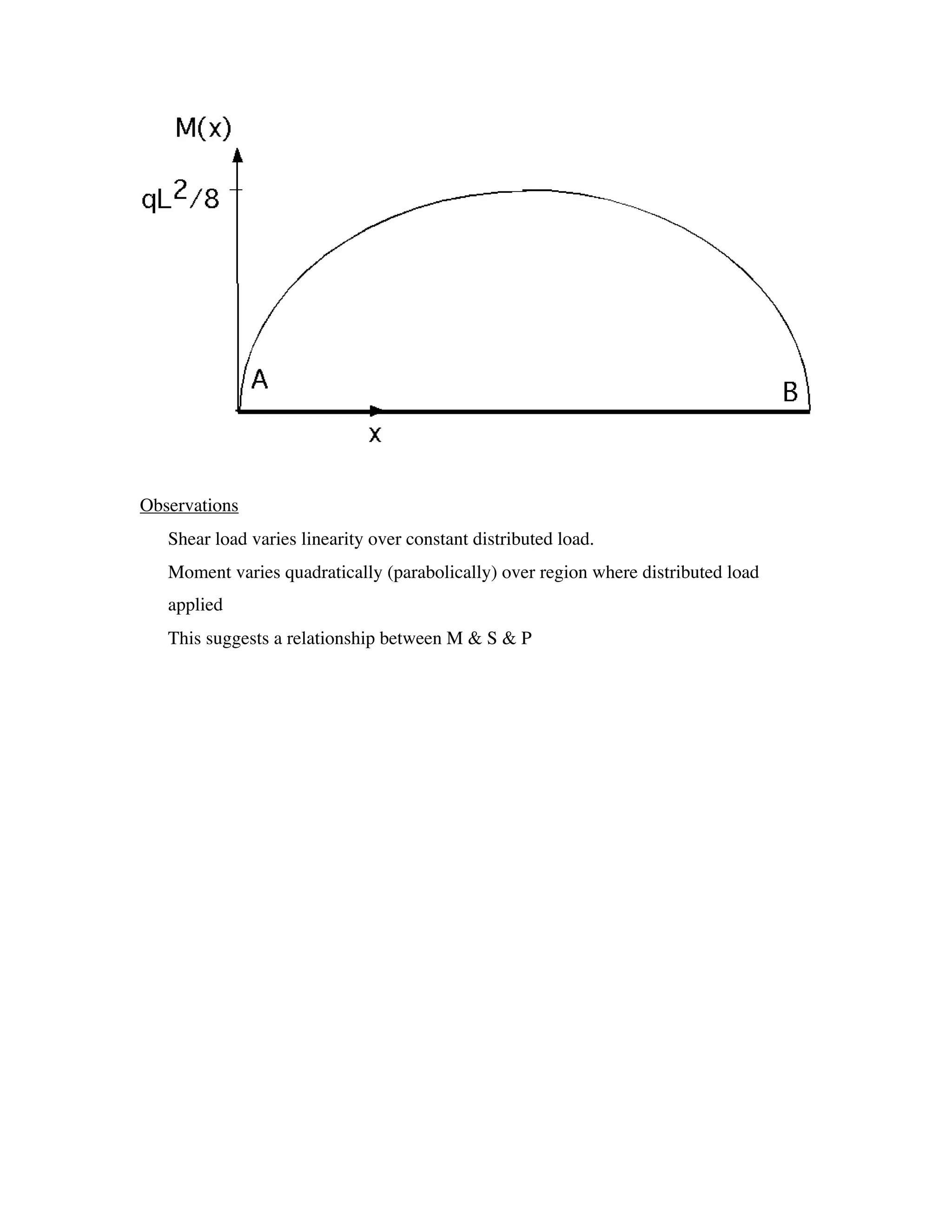
17. Observations
• Shear is constant between point loads
• Bending moment varies linearly between discrete loads.
• Discontinuities occur in S and in slope of M at point of application of concentrated
loads.
• Change in shear equals amount of concentrated loads.
• Values of S & M (and F) go to values of reactions at boundaries
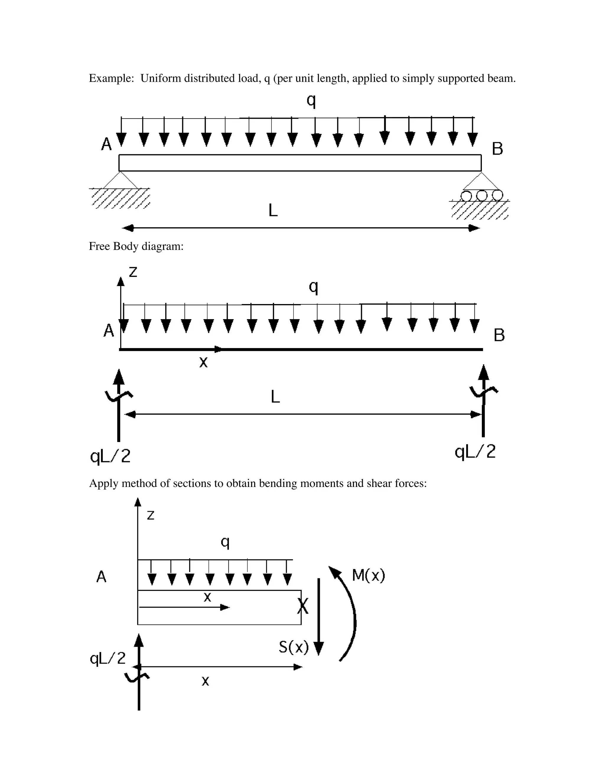
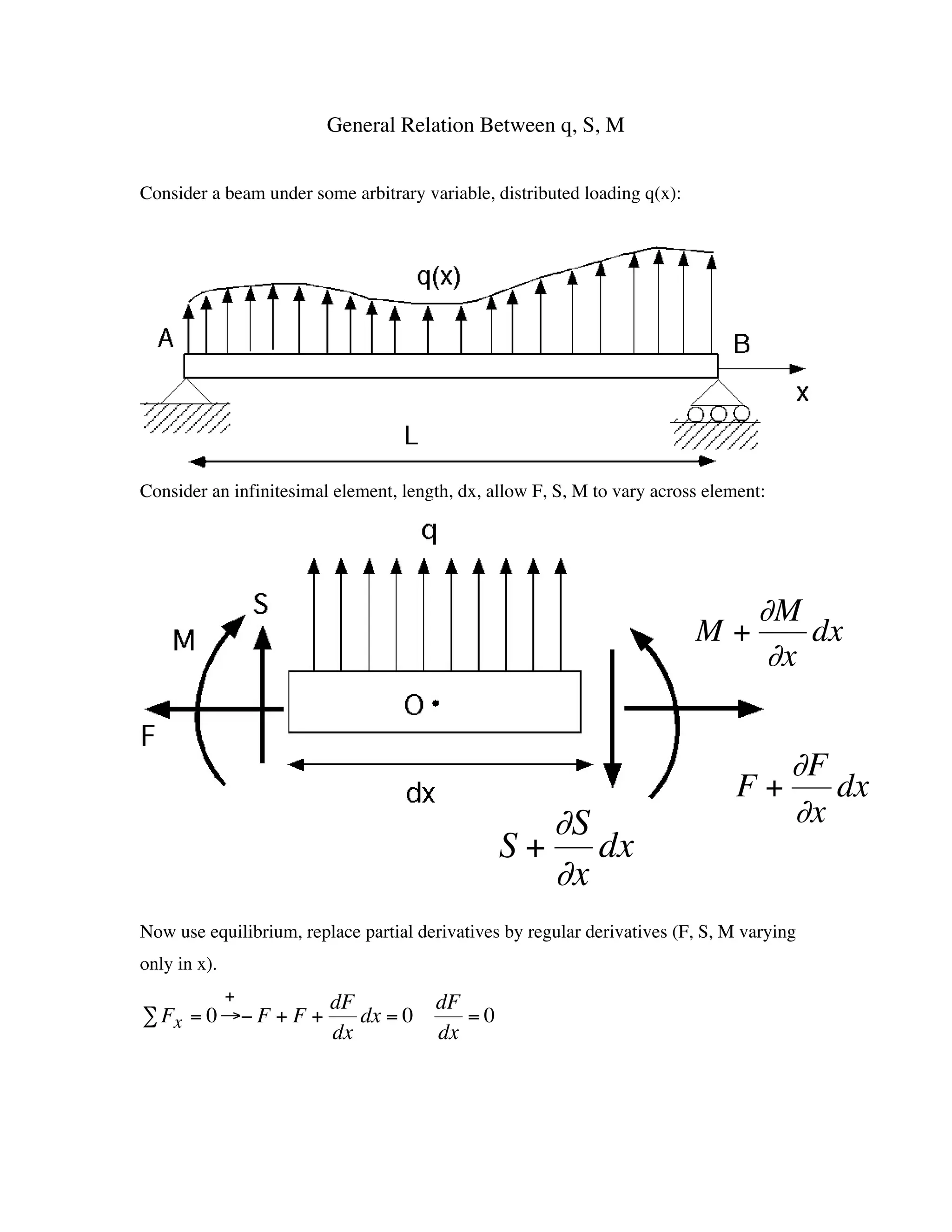
Distributed loads
e.g. gravity, pressure, inertial loading. Can be uniform or varying with position.
Ê x
q(x) = q q(x) = q0 Ë 1- ˆ fi= q0 @ x = 0, = 0@ x = L
L¯
[ q o ] = [force/length]
Deal with distributed loads in essentially the same way as for point loads.

18. Example: Uniform distributed load, q (per unit length, applied to simply supported beam.
Free Body diagram:
Apply method of sections to obtain bending moments and shear forces:

19. Apply equilibrium:
x
qL
Â↑ + - Sx - Ú q dx = 0
2 0
qL
fi - qx = S(x)
2
qLx x
 Mx + - + Mx + Ú qxdx = 0
2 0
qL qx2 qLx qx2
- + Mx = = 0 fi Mx = -
2 2 2 2
Plot:

20. Observations
• Shear load varies linearity over constant distributed load.
• Moment varies quadratically (parabolically) over region where distributed load
applied
• This suggests a relationship between M & S & P

21. General Relation Between q, S, M
Consider a beam under some arbitrary variable, distributed loading q(x):
Consider an infinitesimal element, length, dx, allow F, S, M to vary across element:
∂M
M+ dx
∂x
∂F
† F+ dx
∂S ∂x
S+ dx
∂x
Now use equilibrium, replace partial derivatives by regular derivatives (F, S, M varying
only in x).
†
+ dF dF
 Fx = 0 Æ- F + F + dx = 0 =0
dx† dx
†

22. dS
 Fz = 0 ↑ + S - S - dx + q(x)dx = 0
dx
dS
= q(x)
dx
dM dx dS dx
+ Â M0 -M +M +
/ / dx - S - (S + dx) = 0
† dx 2 dx 2
note: q(x) has no net moment about O.
dM 1 dS
dx - Sdx + (dx) 2 = 0
† dx 2 dx
but (dx) 2 is a higher order (small) term
dM
fi =S
dx
Summarizing:
dF
=0 (unless a bar)
dx
dS
=q
dx
dM d2M
=S (and = q)
dx dx 2
Useful check, useful to automate process
Superposition †
So long as the beam material is elastic and deformations are small all the structural
problems are linear - can use superposition (as for trusses)

23. Lecture M4: Simple Beam Theory
Reading: Crandall, Dahl and Lardner 7.2-7.6
We have looked at the statics of a beam, seen that loads are transmitted by internal
forces: axial forces, shear forces and bending moments.
Now look at how these forces imply stresses, strains, and deflections.
Recall model assumptions: slenderness
General, symmetric, cross section
Geometry
L >> h,b
Loads
Leads to assumptions on stresses
†
s yy = s xy = s yz = 0
Load in x - z plane Æ
Also L >> h,b implies s xx ,s xz >> s zz
†

24. Consider moment equilibrium of a cross section of a beam loaded by some distributed
stress szz, which is reacted by axial stresses on the cross section, sxx
s zz h
 M X = 0 = s zz L - s xx h fi ª ª0
s xx L
i.e. geometry of beam implies sxx >> szz
† Assumptions on Deformations:
The key to simple beam theory is the Bernoulli - Euler hypotheses (1750)
"Plane sections remain plane and perpendicular to the mid-plane after deformation."
It turns out that this is not really an assumption at all but a geometric necessity, at least
for the case of pure bending.
To see what the implications are of this, consider a beam element which undergoes
transverse (bending)
deformation.

25. w= deflection of midplane/midline (function of x only)
Obtain deflection in x-direction, displacement u of point k to K, defined by rotation f .
Note, key assumption, "plane sections remain plane"
†

26. axial displacement, u, of an arbitrary point on the cross-section arises from rotation of
cross, sections
u= -z tanf
Note, negative sign here due to use of consistent definitions of positive directions for w, x
and dw/dx.
If deformations/angles are small tan q ª q
dw dw
fª fi u = -z (1)
dx dx
†
Hence obtain deformation field
dw
u( x, y,z ) = -z
† dx
v( x, y,z ) = 0 nothing happening in y direction
w( x, y,z ) = w( x ) Deflection out of original plane
i.e., cross sections remain rigid (2)
Hence we can obtain distributions of strain. (compatible with deformation). In absence
† of deformations in transverse directions partial derivatives can be replaced by regular
∂_ d_
derivatives, i.e. ≡ . Hence.
∂_ d_
∂u d 2w
e xx = = -z (3)
∂x dx 2
†
∂v ∂w
e yy = = 0, e zz = =0
∂y ∂z
Ê∂u ∂v ˆ Ê∂v ∂w ˆ
g xy = 2e12 = Á + ˜ = 0, g yz = Á + ˜ = 0
Ë ∂y ∂x ¯ Ë∂z ∂y ¯
Ê∂u ∂w ˆ Ê dw dw ˆ
g xz = Á + ˜ = Á- + ˜=0
Ë ∂z ∂x ¯ Ë dx dx ¯
If no shear - consistent with B-E assumption of plane sections remaining plane.
dM
for constant bending moment: =S=0 (will revisit for S ≠ 0)
† dx

27. Next use stress - strain (assume orthotropic - for generality)
s xx (4)
e xx =
Ex
s xx
e yy = -n xy
Ex
s
e zz = -n xz xx
Ex
t xy
g xy =
G xy
t yz
g yz = Note inconsistency -
G yz g xz = 0, t xz ≠ 0 (shear
t forces are non zero)
g xz = xz
G xz
†
The inconsistency on the shear stress/strain arises from the plane/sections remain plane
assumption. Does not strictly apply when there is varying bending moment (and hence
†
non-zero shear force). However, displacements due to g xz are very small compared to
those due to e xx , and therefore negligible.
†
Finally apply equilibrium:
† ∂s mn
+ fm = 0
∂x m
(5)
∂s xx ∂s yz ∂s zx ∂s xx ∂szx
+ + =0fi + =0
∂x ∂y ∂z ∂x ∂z
∂s xy ∂s yy ∂s zy
+ + =0 fi0=0
∂x ∂y ∂z
∂s xz ∂s yz ∂s zz ∂s xz
+ + =0fi =0
∂x ∂y ∂y ∂z
5 equations, 5 unknowns : w,u,e xx ,s xx ,s xz
To be continued…
†
†