Download as PDF, PPTX
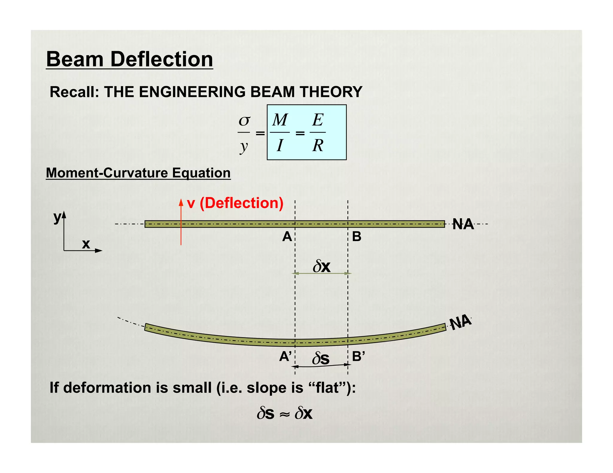
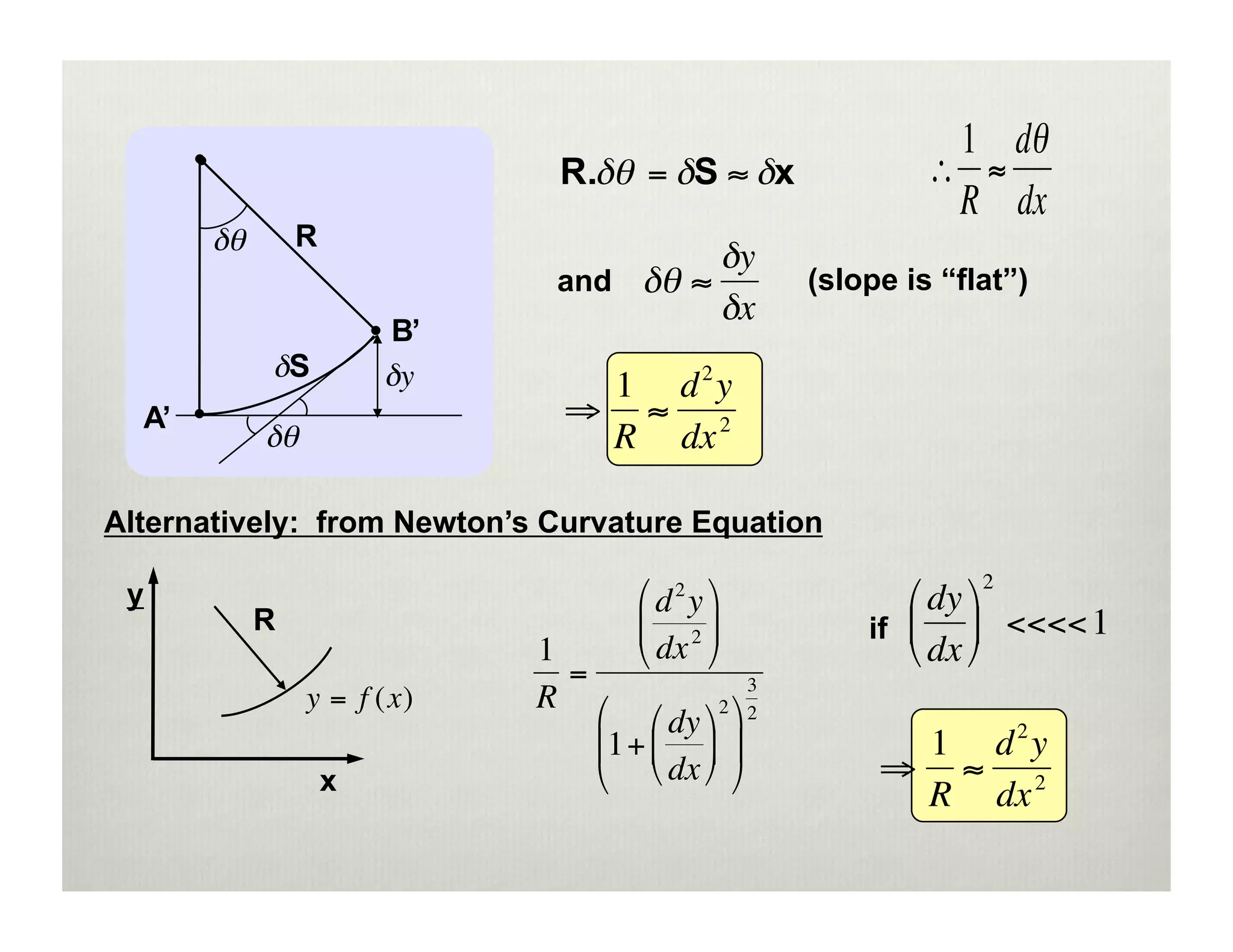
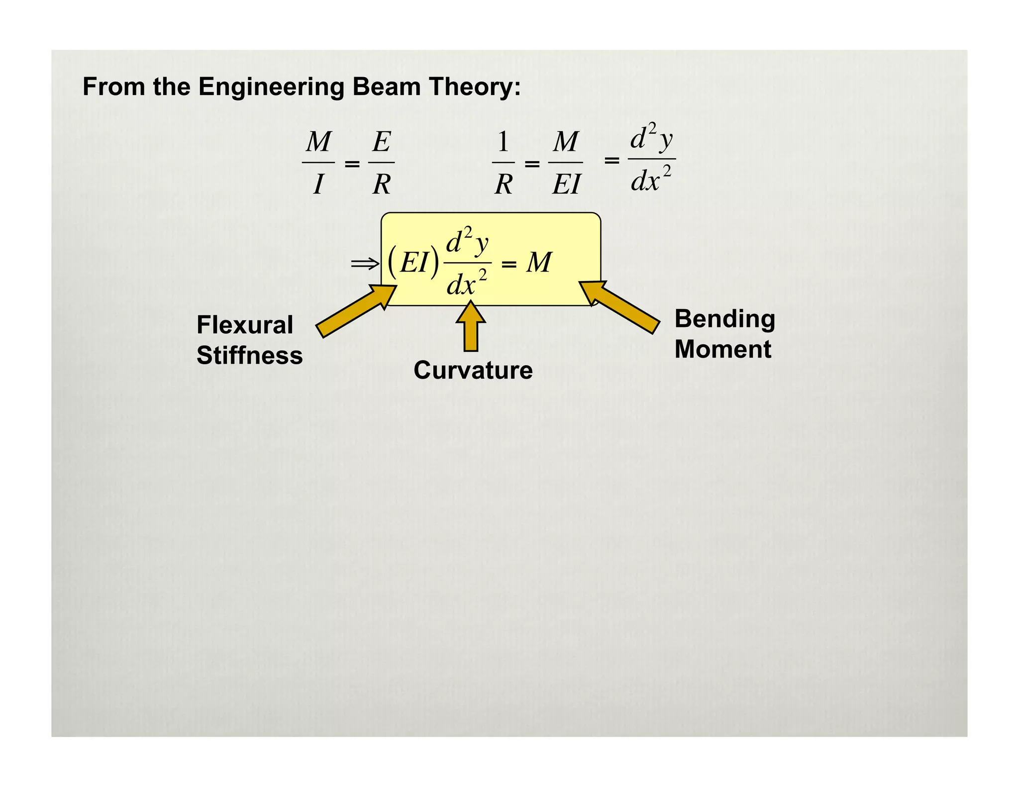
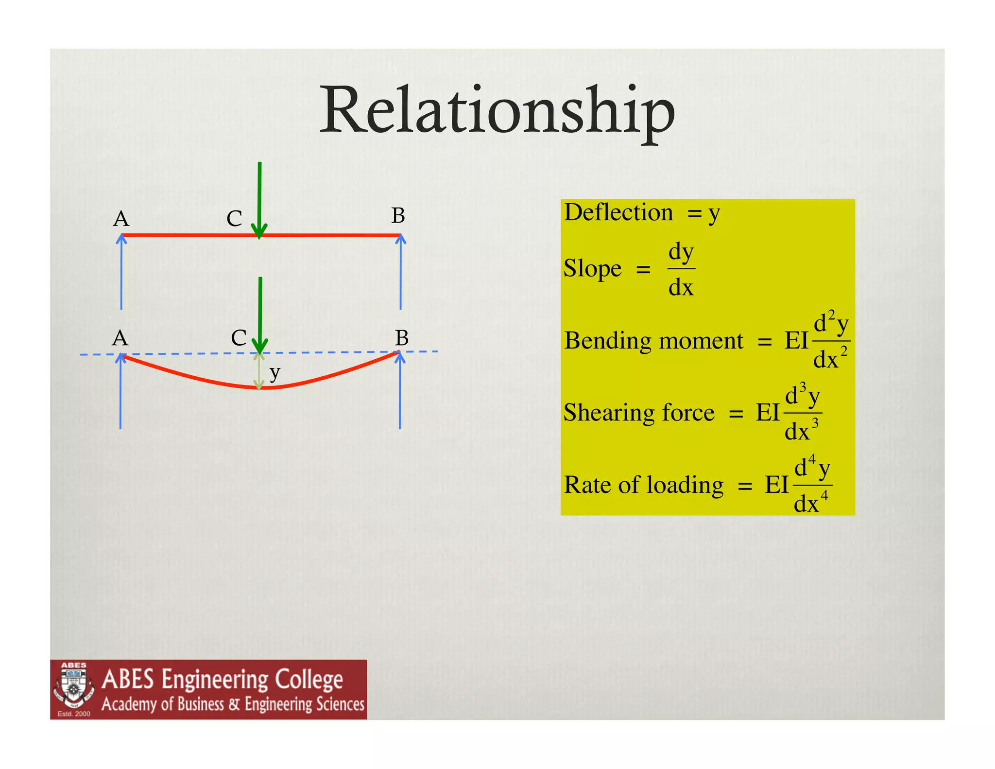
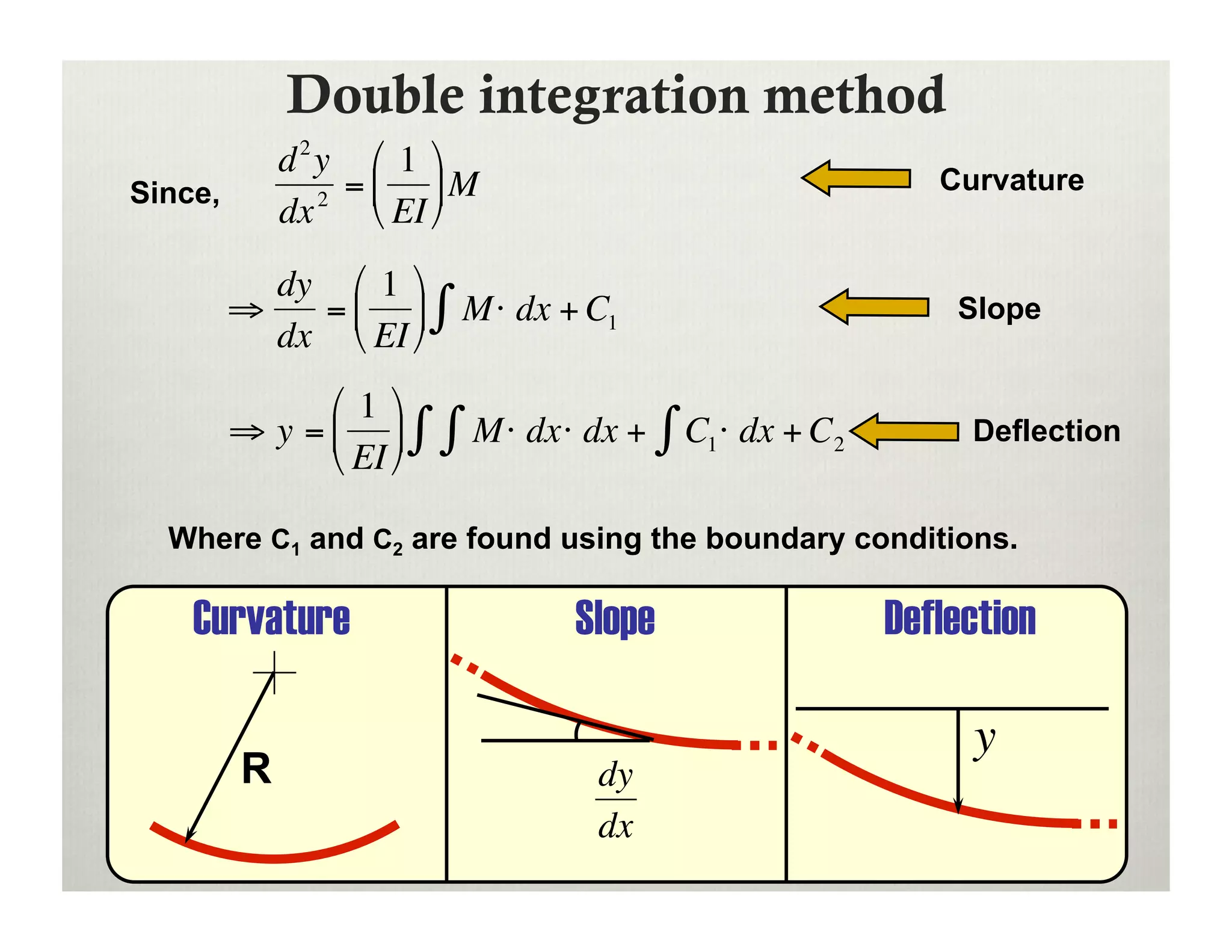
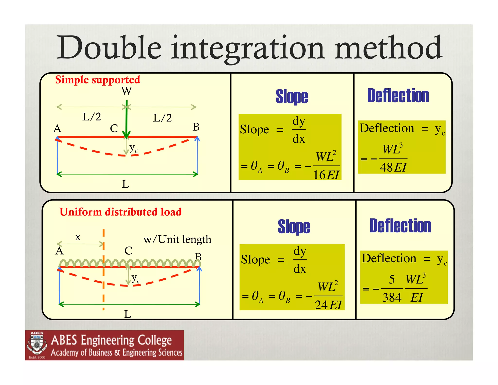
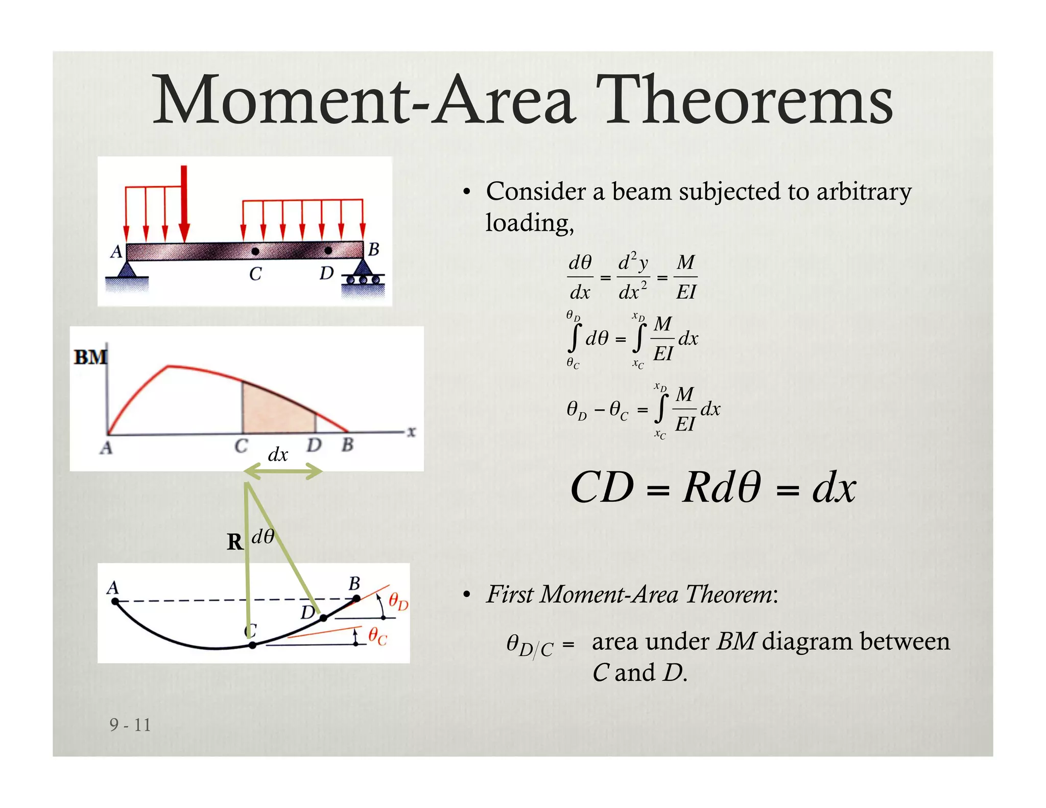
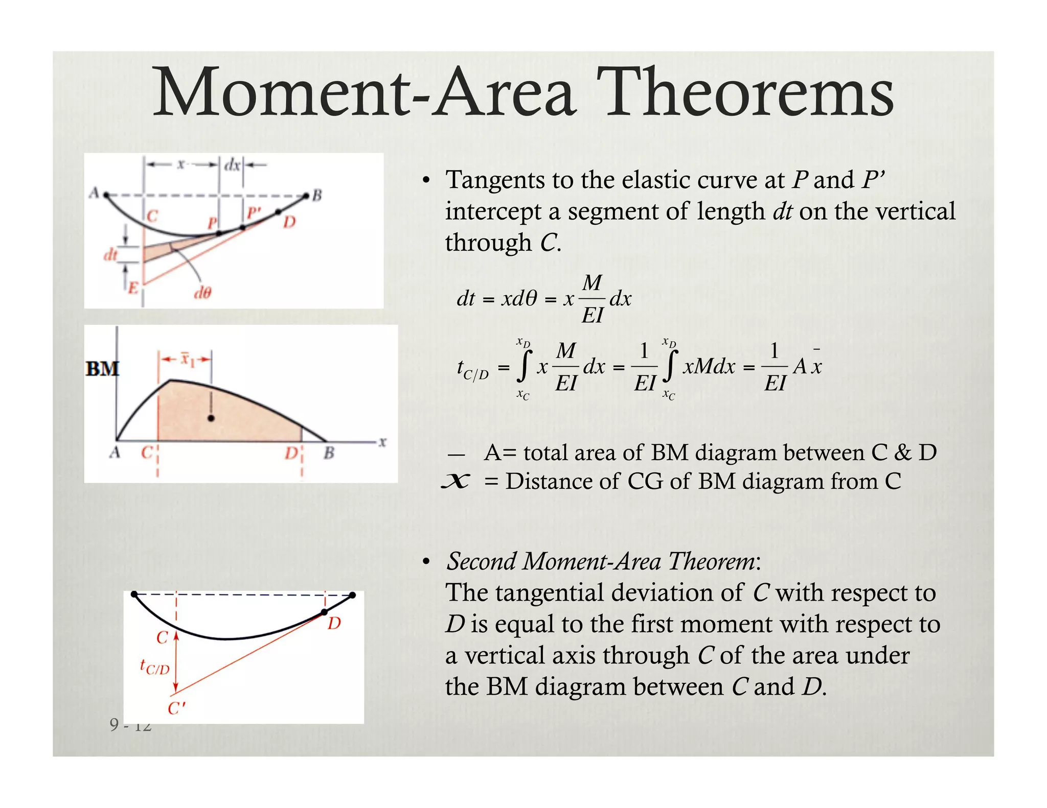

This document discusses stresses in beams and beam deflection. It covers several methods for analyzing bending stresses and deflection in beams, including: [1] the engineering beam theory relating moment, curvature, and stress; [2] double integration and moment area methods for calculating slope and deflection; and [3] Macaulay's method, which simplifies calculations for beams with eccentric loads. Formulas are provided relating bending moment, shear force, curvature, slope, and deflection. Moment-area theorems are also described for relating bending moment to slope and deflection.
Introduction to Unit 2 covering shear force, bending moment diagrams, stresses and deflection in beams.
Discussion of beam deflection, engineering beam theory, moment-curvature relationship, and bending moment equation.
Presentation of methods for calculating slope and deflection including double integration and Macaulay’s method.
Introduction of Moment-Area Theorems to evaluate deflections using the area under the bending moment diagram.
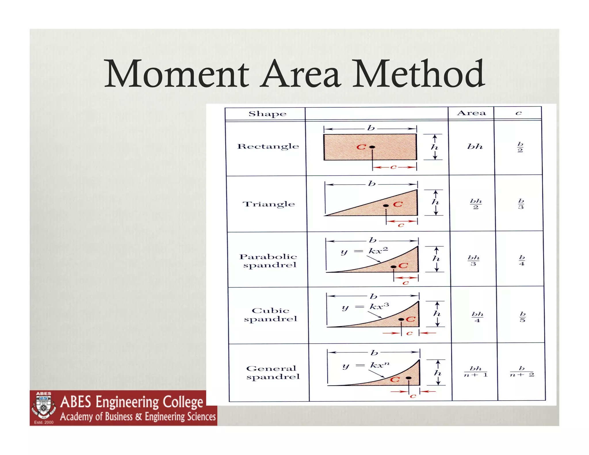
Elaboration on the Moment Area Method for finding shear and deflection in beams.
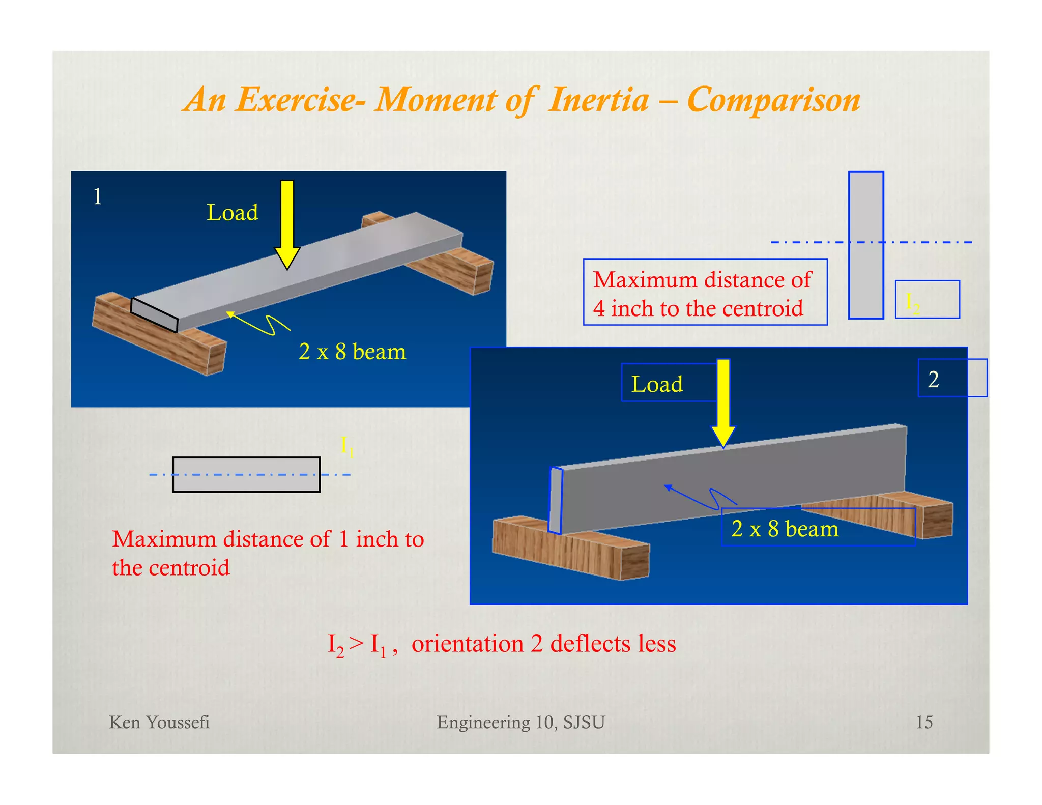
An exercise comparing the moment of inertia of beams and their deflection characteristics.


