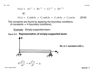
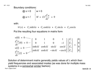
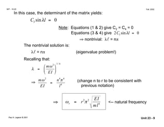
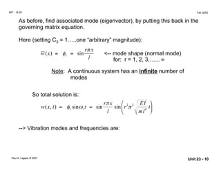
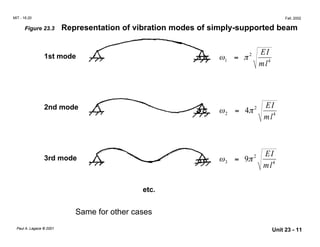
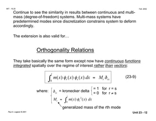
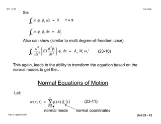
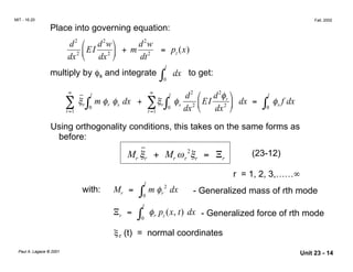
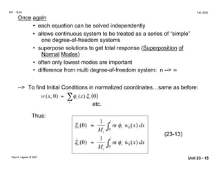
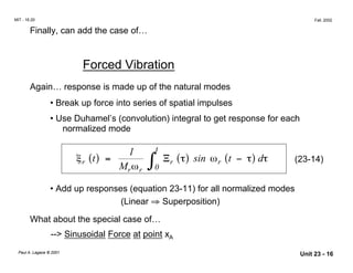
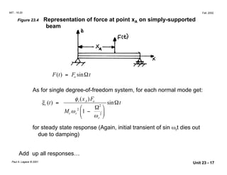
MIT - 16.20 Fall, 2002
Unit 23

Vibration of Continuous Systems

Paul A. Lagace, Ph.D.

Professor of Aeronautics & Astronautics

and Engineering Systems

Paul A. Lagace © 2001
MIT - 16.20 Fall, 2002
The logical extension of discrete mass systems is one of an
infinite number of masses. In the limit, this is a continuous
system.
Take the generalized beam-column as a generic representation:
2
d2

EI
d w
dx2 
 dx2

 −
d 
F
d w


= pz (23-1)
dx  dx 
Figure 23.1 Representation of generalized beam-column
d F
= − px
dx
This considers only static loads. Must add the inertial load(s). Since the
concern is in the z-displacement (w):
˙˙Inertial load unit length = mw (23-2)
where: m(x) = mass/unit length
Paul A. Lagace © 2001 Unit 23 - 2
w
MIT - 16.20
 Fall, 2002
Use per unit length since entire equation is of this form. Thus:
2

d2

EI
d w

dx2 
 dx2

 −
d 
F
d w


= pz − m ˙˙

dx  dx 
or:
2

d2

EI
d w
˙˙

dx2 
 dx2

 −
d 
F
d w


+ mw = pz (23-3)

dx  dx 
Beam Bending Equation
often, F = 0 and this becomes:
2

d2
2

EI
d w
+ mw = pz
dx  dx2 

˙˙
--> This is a fourth order differential equation in x

--> Need four boundary conditions
--> This is a second order differential equation in time
--> Need two initial conditions
Paul A. Lagace © 2001
 Unit 23 - 3
w
i t
MIT - 16.20 Fall, 2002
Notes:
• Could also get via simple beam equations. Change occurs in:
d S
= pz − m ˙˙
dx
• If consider dynamics along x, must include mu˙˙ in px term: ( px − mu˙˙)
Use the same approach as in the discrete spring-mass systems:
Free Vibration
Again assume harmonic motion. In a continuous system, there are an
infinite number of natural frequencies (eigenvalues) and associated
modes (eigenvectors)
so:
ω
w x( , t) = w (x) e
separable solution spatially (x) and temporally (t)
Consider the homogeneous case (pz = 0) and let there be no axial forces
(px = 0 ⇒ F = 0)
Paul A. Lagace © 2001 Unit 23 - 4
i t i t
MIT - 16.20
 Fall, 2002
So:
2

d2

EI
d w
+ mw = 0
dx2 
 dx2 

˙˙
Also assume that EI does not vary with x:
4

˙˙EI
d w
+ mw = 0 (23-5)

dx4

Placing the assumed mode in the governing equation:
4

EI
d w
e ω
− mω2
w e ω
= 0

dx4

This gives:
4

EI
d w
− mω2
w = 0 (23-6)

dx4

which is now an equation solely in the spatial variable (successful
separation of t and x dependencies)
_
Must now find a solution for w(x) which satisfies the differential equations
and the boundary conditions.
Note: the shape and frequency are intimately linked
(through equation 23-6)
Paul A. Lagace © 2001

Unit 23 - 5
MIT - 16.20 Fall, 2002
Can recast equation (23-6) to be:
4
d w mω2
dx4
− w = 0 (23-7)
EI
The solution to this homogeneous equation is of the form:
w x( ) = e p x
Putting this into (23-7) yields
4 p x mω2
p e − e p x
= 0
EI
4 mω2
⇒	 p =
EI
So this is an eigenvalue problem (spatially). The four roots are:
p = +λ, -λ, + iλ, - iλ
where:
1 4
 mω2

/
λ =  
 EI 
This yields:
Paul A. Lagace © 2001
Unit 23 - 6
MIT - 16.20 Fall, 2002
λ
w x( ) = Ae λ x
+ Be −λ x
+ Cei λ x
+ De −i x
or:
w x( ) = C1 sinhλx + C2 coshλx + C3 sinλx + C4 cosλx (23-8)
The constants are found by applying the boundary conditions
(4 constants ⇒ 4 boundary conditions)
Example: Simply-supported beam
Figure 23.2 Representation of simply-supported beam
EI, m = constant with x
4 2
EI
d w
+ m
d w
= pz
dx4
dt2
Paul A. Lagace © 2001 Unit 23 - 7
MIT - 16.20 Fall, 2002
Boundary conditions:
@ x = 0 w = 0
2
@ x = l M = EI
d w
= 0
dx2
with:
w x( ) = C1 sinhλx + C2 coshλx + C3 sinλx + C4 cosλx
Put the resulting four equations in matrix form
w 0
2
( ) = 0
 0 1 0 1  C1  0
d w
dx2 ( ) = 0 

0 1 0 −1     0 C2  0   =  
( ) = 0 sinhλl coshλl sinλl cosλl  C3  0w l
d w 
sinhλl coshλl −sinλl −cosλl
 C4  02    
l
dx2 ( ) = 0
Solution of determinant matrix generally yields values of λ which then
yield frequencies and associated modes (as was done for multiple mass
systems in a somewhat similar fashion)
Paul A. Lagace © 2001 Unit 23 - 8
MIT - 16.20 Fall, 2002
In this case, the determinant of the matrix yields:
C sinλl = 03
Note: 	Equations (1 & 2) give C2 = C4 = 0
Equations (3 & 4) give 2C3 sinλl = 0
⇒ nontrivial: λl = nπ
The nontrivial solution is:
λl = nπ (eigenvalue problem!)
Recalling that:
1 4
 mω2

/
λ =  
 EI 
4
mω2
n π4
(change n to r to be consistent with⇒	 =
EI l4
previous notation)
2 2
⇒ ωr = r π
EI
ml4 <-- natural frequency
Paul A. Lagace © 2001 Unit 23 - 9
r x
r x
MIT - 16.20 Fall, 2002
As before, find associated mode (eigenvector), by putting this back in the
governing matrix equation.
Here (setting C3 = 1…..one “arbitrary” magnitude):
π
w x( ) = φr = sin <-- mode shape (normal mode)
l for: r = 1, 2, 3,……∞
Note: A continuous system has an infinite number of
modes
So total solution is:
π  2 2 EI
ml4

w x( , t) = φr sinωrt = sin sinr π tl  
--> Vibration modes and frequencies are:
Paul A. Lagace © 2001
Unit 23 - 10
MIT - 16.20 Fall, 2002
Figure 23.3 Representation of vibration modes of simply-supported beam
1st mode ω = π2
1 4
EI
ml
2nd mode ω = 4π2
2 4
EI
ml
3rd mode ω = 9π2
3 4
EI
ml
etc.
Same for other cases
Paul A. Lagace © 2001 Unit 23 - 11
MIT - 16.20 Fall, 2002
Continue to see the similarity in results between continuous and multi-
mass (degree-of-freedom) systems. Multi-mass systems have
predetermined modes since discretization constrains system to deform
accordingly.
The extension is also valid for…
Orthogonality Relations
They take basically the same form except now have continuous functions
integrated spatially over the regime of interest rather than vectors:
l
∫0
m x x x( ) φr ( ) φs ( ) dx = Mr δrs
(23-9)
= 1 for r = s
where: δrs
= kronecker delta
= 0 for r ≠ s
l
( ) φr
2
( ) dxMr = ∫0
m x x
generalized mass of the rth mode
Paul A. Lagace © 2001 Unit 23 - 12
MIT - 16.20 Fall, 2002
So:
l
∫0
m φ φs dx = 0 r ≠ sr
l
∫0
m φ φr dx = Mrr
Also can show (similar to multi degree-of-freedom case):
2
l d2


EI
d
dx
φ
2
r 

 φs dx = δrs Mr ωr
2
(23-10)∫0 dx2

This again, leads to the ability to transform the equation based on the
normal modes to get the…
Normal Equations of Motion
Let:
∞
w x( , t) = ∑φr (x) ξr ( )t (23-11)
r =1
normal mode normal coordinates
Paul A. Lagace © 2001 Unit 23 - 13
p x
p x
MIT - 16.20 Fall, 2002
Place into governing equation:
2 2
d2
2

EI
d w
+ m
d w
= z ( )
dx  dx2 
 dt2
l
multiply by φs and integrate ∫0
dx to get:
∞
˙˙
∞
d2
 2
∑ ξr ∫0
l
m φr φs dx + ∑ξr ∫0
l
φs
dx2

EI
d
dx
φ
2
r 


dx = ∫0
l
φs f dx
r=1 r=1
Using orthogonality conditions, this takes on the same forms as
before:
˙˙M ξ + M ω 2
ξ = Ξ (23-12)r r r r r r
r = 1, 2, 3,……∞
l
with: Mr = ∫0
m φr
2
dx - Generalized mass of rth mode
l
Ξr = ∫0
φr z ( , t) dx - Generalized force of rth mode
ξr (t) = normal coordinates
Paul A. Lagace © 2001
Unit 23 - 14
MIT - 16.20 Fall, 2002
Once again
• each equation can be solved independently
• 	allows continuous system to be treated as a series of “simple”
one degree-of-freedom systems
• 	superpose solutions to get total response (Superposition of
Normal Modes)
• often only lowest modes are important
• difference from multi degree-of-freedom system: n --> ∞
--> To find Initial Conditions in normalized coordinates…same as before:
( , 0) = ∑φr (x) ξr ( )w x 0
r
etc.
Thus:
1 l
0ξr ( ) =
M ∫0
m φr w0 (x) dx
r
(23-13)
˙
r ( ) =
1
∫0
l
m φr w˙0 ( ) dxξ 0 x
Mr
Paul A. Lagace © 2001
Unit 23 - 15
MIT - 16.20 Fall, 2002
Finally, can add the case of…
Forced Vibration
Again… response is made up of the natural modes
• Break up force into series of spatial impulses
• Use Duhamel’s (convolution) integral to get response for each
normalized mode
ξ
ω
τ τ τr
r r
rt
M
t
t
( ) = ( ) −( )∫
1
0
Ξ sin ωr d (23-14)
• Add up responses (equation 23-11) for all normalized modes
(Linear ⇒ Superposition)
What about the special case of…
--> Sinusoidal Force at point xA
Paul A. Lagace © 2001 Unit 23 - 16
x F
MIT - 16.20 Fall, 2002
Figure 23.4 Representation of force at point xA on simply-supported
beam
F t( ) = Fo sinΩt
As for single degree-of-freedom system, for each normal mode get:
t A
ξr ( ) =
φr ( ) o
2
sinΩt
Mr ωr
2


1 −
Ω
2 

 ω r
for steady state response (Again, initial transient of sin ωrt dies out
due to damping)
Add up all responses…
Paul A. Lagace © 2001 Unit 23 - 17
MIT - 16.20 Fall, 2002
Note:

• Resonance can occur at any ωr
• DMF (Dynamic Magnification Factor) associated with each normal
mode
--> Can apply technique to any system.
• Get governing equation including inertial terms
• Determine Free Vibration Modes and frequencies
• Transform equation to uncoupled single degree-of-freedom system
(normal equations)
• Solve each normal equation separately
• Total response equal to sum of individual responses
Modal superposition is a very powerful technique!
Paul A. Lagace © 2001 Unit 23 - 18

Unit23

  • 1.
    MIT - 16.20Fall, 2002 Unit 23 Vibration of Continuous Systems Paul A. Lagace, Ph.D. Professor of Aeronautics & Astronautics and Engineering Systems Paul A. Lagace © 2001
  • 2.
    MIT - 16.20Fall, 2002 The logical extension of discrete mass systems is one of an infinite number of masses. In the limit, this is a continuous system. Take the generalized beam-column as a generic representation: 2 d2  EI d w dx2   dx2   − d  F d w   = pz (23-1) dx  dx  Figure 23.1 Representation of generalized beam-column d F = − px dx This considers only static loads. Must add the inertial load(s). Since the concern is in the z-displacement (w): ˙˙Inertial load unit length = mw (23-2) where: m(x) = mass/unit length Paul A. Lagace © 2001 Unit 23 - 2
  • 3.
    w MIT - 16.20 Fall, 2002 Use per unit length since entire equation is of this form. Thus: 2 d2  EI d w dx2   dx2   − d  F d w   = pz − m ˙˙ dx  dx  or: 2 d2  EI d w ˙˙ dx2   dx2   − d  F d w   + mw = pz (23-3) dx  dx  Beam Bending Equation often, F = 0 and this becomes: 2 d2 2  EI d w + mw = pz dx  dx2   ˙˙ --> This is a fourth order differential equation in x --> Need four boundary conditions --> This is a second order differential equation in time --> Need two initial conditions Paul A. Lagace © 2001 Unit 23 - 3
  • 4.
    w i t MIT -16.20 Fall, 2002 Notes: • Could also get via simple beam equations. Change occurs in: d S = pz − m ˙˙ dx • If consider dynamics along x, must include mu˙˙ in px term: ( px − mu˙˙) Use the same approach as in the discrete spring-mass systems: Free Vibration Again assume harmonic motion. In a continuous system, there are an infinite number of natural frequencies (eigenvalues) and associated modes (eigenvectors) so: ω w x( , t) = w (x) e separable solution spatially (x) and temporally (t) Consider the homogeneous case (pz = 0) and let there be no axial forces (px = 0 ⇒ F = 0) Paul A. Lagace © 2001 Unit 23 - 4
  • 5.
    i t it MIT - 16.20 Fall, 2002 So: 2 d2  EI d w + mw = 0 dx2   dx2   ˙˙ Also assume that EI does not vary with x: 4 ˙˙EI d w + mw = 0 (23-5) dx4 Placing the assumed mode in the governing equation: 4 EI d w e ω − mω2 w e ω = 0 dx4 This gives: 4 EI d w − mω2 w = 0 (23-6) dx4 which is now an equation solely in the spatial variable (successful separation of t and x dependencies) _ Must now find a solution for w(x) which satisfies the differential equations and the boundary conditions. Note: the shape and frequency are intimately linked (through equation 23-6) Paul A. Lagace © 2001 Unit 23 - 5
  • 6.
    MIT - 16.20Fall, 2002 Can recast equation (23-6) to be: 4 d w mω2 dx4 − w = 0 (23-7) EI The solution to this homogeneous equation is of the form: w x( ) = e p x Putting this into (23-7) yields 4 p x mω2 p e − e p x = 0 EI 4 mω2 ⇒ p = EI So this is an eigenvalue problem (spatially). The four roots are: p = +λ, -λ, + iλ, - iλ where: 1 4  mω2  / λ =    EI  This yields: Paul A. Lagace © 2001 Unit 23 - 6
  • 7.
    MIT - 16.20Fall, 2002 λ w x( ) = Ae λ x + Be −λ x + Cei λ x + De −i x or: w x( ) = C1 sinhλx + C2 coshλx + C3 sinλx + C4 cosλx (23-8) The constants are found by applying the boundary conditions (4 constants ⇒ 4 boundary conditions) Example: Simply-supported beam Figure 23.2 Representation of simply-supported beam EI, m = constant with x 4 2 EI d w + m d w = pz dx4 dt2 Paul A. Lagace © 2001 Unit 23 - 7
  • 8.
    MIT - 16.20Fall, 2002 Boundary conditions: @ x = 0 w = 0 2 @ x = l M = EI d w = 0 dx2 with: w x( ) = C1 sinhλx + C2 coshλx + C3 sinλx + C4 cosλx Put the resulting four equations in matrix form w 0 2 ( ) = 0  0 1 0 1  C1  0 d w dx2 ( ) = 0   0 1 0 −1     0 C2  0   =   ( ) = 0 sinhλl coshλl sinλl cosλl  C3  0w l d w  sinhλl coshλl −sinλl −cosλl  C4  02     l dx2 ( ) = 0 Solution of determinant matrix generally yields values of λ which then yield frequencies and associated modes (as was done for multiple mass systems in a somewhat similar fashion) Paul A. Lagace © 2001 Unit 23 - 8
  • 9.
    MIT - 16.20Fall, 2002 In this case, the determinant of the matrix yields: C sinλl = 03 Note: Equations (1 & 2) give C2 = C4 = 0 Equations (3 & 4) give 2C3 sinλl = 0 ⇒ nontrivial: λl = nπ The nontrivial solution is: λl = nπ (eigenvalue problem!) Recalling that: 1 4  mω2  / λ =    EI  4 mω2 n π4 (change n to r to be consistent with⇒ = EI l4 previous notation) 2 2 ⇒ ωr = r π EI ml4 <-- natural frequency Paul A. Lagace © 2001 Unit 23 - 9
  • 10.
    r x r x MIT- 16.20 Fall, 2002 As before, find associated mode (eigenvector), by putting this back in the governing matrix equation. Here (setting C3 = 1…..one “arbitrary” magnitude): π w x( ) = φr = sin <-- mode shape (normal mode) l for: r = 1, 2, 3,……∞ Note: A continuous system has an infinite number of modes So total solution is: π  2 2 EI ml4  w x( , t) = φr sinωrt = sin sinr π tl   --> Vibration modes and frequencies are: Paul A. Lagace © 2001 Unit 23 - 10
  • 11.
    MIT - 16.20Fall, 2002 Figure 23.3 Representation of vibration modes of simply-supported beam 1st mode ω = π2 1 4 EI ml 2nd mode ω = 4π2 2 4 EI ml 3rd mode ω = 9π2 3 4 EI ml etc. Same for other cases Paul A. Lagace © 2001 Unit 23 - 11
  • 12.
    MIT - 16.20Fall, 2002 Continue to see the similarity in results between continuous and multi- mass (degree-of-freedom) systems. Multi-mass systems have predetermined modes since discretization constrains system to deform accordingly. The extension is also valid for… Orthogonality Relations They take basically the same form except now have continuous functions integrated spatially over the regime of interest rather than vectors: l ∫0 m x x x( ) φr ( ) φs ( ) dx = Mr δrs (23-9) = 1 for r = s where: δrs = kronecker delta = 0 for r ≠ s l ( ) φr 2 ( ) dxMr = ∫0 m x x generalized mass of the rth mode Paul A. Lagace © 2001 Unit 23 - 12
  • 13.
    MIT - 16.20Fall, 2002 So: l ∫0 m φ φs dx = 0 r ≠ sr l ∫0 m φ φr dx = Mrr Also can show (similar to multi degree-of-freedom case): 2 l d2   EI d dx φ 2 r    φs dx = δrs Mr ωr 2 (23-10)∫0 dx2  This again, leads to the ability to transform the equation based on the normal modes to get the… Normal Equations of Motion Let: ∞ w x( , t) = ∑φr (x) ξr ( )t (23-11) r =1 normal mode normal coordinates Paul A. Lagace © 2001 Unit 23 - 13
  • 14.
    p x p x MIT- 16.20 Fall, 2002 Place into governing equation: 2 2 d2 2  EI d w + m d w = z ( ) dx  dx2   dt2 l multiply by φs and integrate ∫0 dx to get: ∞ ˙˙ ∞ d2  2 ∑ ξr ∫0 l m φr φs dx + ∑ξr ∫0 l φs dx2  EI d dx φ 2 r    dx = ∫0 l φs f dx r=1 r=1 Using orthogonality conditions, this takes on the same forms as before: ˙˙M ξ + M ω 2 ξ = Ξ (23-12)r r r r r r r = 1, 2, 3,……∞ l with: Mr = ∫0 m φr 2 dx - Generalized mass of rth mode l Ξr = ∫0 φr z ( , t) dx - Generalized force of rth mode ξr (t) = normal coordinates Paul A. Lagace © 2001 Unit 23 - 14
  • 15.
    MIT - 16.20Fall, 2002 Once again • each equation can be solved independently • allows continuous system to be treated as a series of “simple” one degree-of-freedom systems • superpose solutions to get total response (Superposition of Normal Modes) • often only lowest modes are important • difference from multi degree-of-freedom system: n --> ∞ --> To find Initial Conditions in normalized coordinates…same as before: ( , 0) = ∑φr (x) ξr ( )w x 0 r etc. Thus: 1 l 0ξr ( ) = M ∫0 m φr w0 (x) dx r (23-13) ˙ r ( ) = 1 ∫0 l m φr w˙0 ( ) dxξ 0 x Mr Paul A. Lagace © 2001 Unit 23 - 15
  • 16.
    MIT - 16.20Fall, 2002 Finally, can add the case of… Forced Vibration Again… response is made up of the natural modes • Break up force into series of spatial impulses • Use Duhamel’s (convolution) integral to get response for each normalized mode ξ ω τ τ τr r r rt M t t ( ) = ( ) −( )∫ 1 0 Ξ sin ωr d (23-14) • Add up responses (equation 23-11) for all normalized modes (Linear ⇒ Superposition) What about the special case of… --> Sinusoidal Force at point xA Paul A. Lagace © 2001 Unit 23 - 16
  • 17.
    x F MIT -16.20 Fall, 2002 Figure 23.4 Representation of force at point xA on simply-supported beam F t( ) = Fo sinΩt As for single degree-of-freedom system, for each normal mode get: t A ξr ( ) = φr ( ) o 2 sinΩt Mr ωr 2   1 − Ω 2    ω r for steady state response (Again, initial transient of sin ωrt dies out due to damping) Add up all responses… Paul A. Lagace © 2001 Unit 23 - 17
  • 18.
    MIT - 16.20Fall, 2002 Note: • Resonance can occur at any ωr • DMF (Dynamic Magnification Factor) associated with each normal mode --> Can apply technique to any system. • Get governing equation including inertial terms • Determine Free Vibration Modes and frequencies • Transform equation to uncoupled single degree-of-freedom system (normal equations) • Solve each normal equation separately • Total response equal to sum of individual responses Modal superposition is a very powerful technique! Paul A. Lagace © 2001 Unit 23 - 18