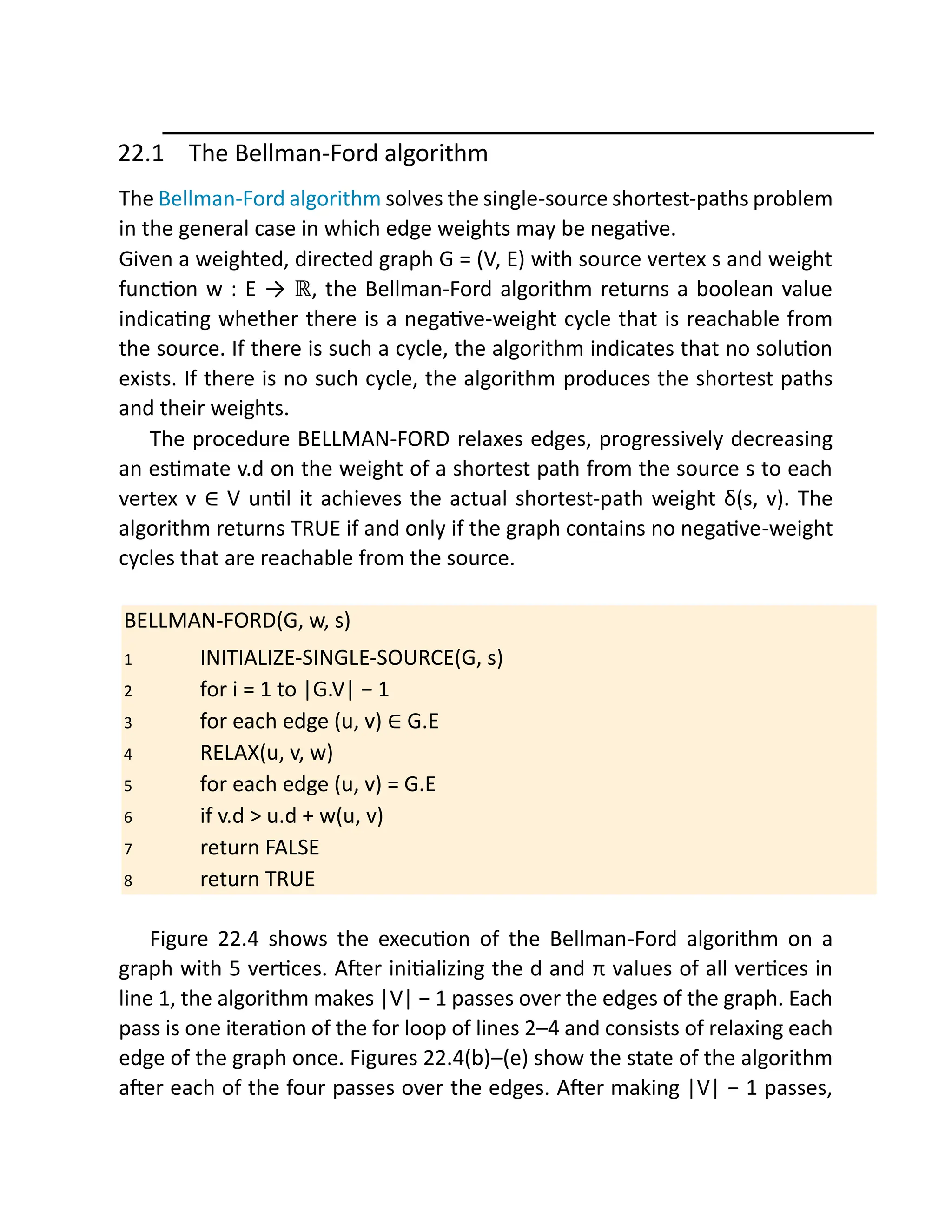
The Bellman-Ford algorithm solves the single-source shortest-path problem for weighted directed graphs, even with negative edge weights, by detecting negative-weight cycles and computing shortest paths. It operates with a time complexity of O(V^2 + VE) and guarantees correct shortest-path weights if no negative cycles are reachable from the source. Additionally, the document discusses the dag-shortest-paths algorithm for directed acyclic graphs, which efficiently computes shortest paths in linear time.

1. 22.1 The Bellman-Ford algorithm
The Bellman-Ford algorithm solves the single-source shortest-paths problem
in the general case in which edge weights may be negative.
Given a weighted, directed graph G = (V, E) with source vertex s and weight
function w : E → ℝ, the Bellman-Ford algorithm returns a boolean value
indicating whether there is a negative-weight cycle that is reachable from
the source. If there is such a cycle, the algorithm indicates that no solution
exists. If there is no such cycle, the algorithm produces the shortest paths
and their weights.
The procedure BELLMAN-FORD relaxes edges, progressively decreasing
an estimate v.d on the weight of a shortest path from the source s to each
vertex v ∈ V until it achieves the actual shortest-path weight δ(s, v). The
algorithm returns TRUE if and only if the graph contains no negative-weight
cycles that are reachable from the source.
BELLMAN-FORD(G, w, s)
1 INITIALIZE-SINGLE-SOURCE(G, s)
2 for i = 1 to |G.V| − 1
3 for each edge (u, v) ∈ G.E
4 RELAX(u, v, w)
5 for each edge (u, v) = G.E
6 if v.d > u.d + w(u, v)
7 return FALSE
8 return TRUE
Figure 22.4 shows the execution of the Bellman-Ford algorithm on a
graph with 5 vertices. After initializing the d and π values of all vertices in
line 1, the algorithm makes |V| − 1 passes over the edges of the graph. Each
pass is one iteration of the for loop of lines 2–4 and consists of relaxing each
edge of the graph once. Figures 22.4(b)–(e) show the state of the algorithm
after each of the four passes over the edges. After making |V| − 1 passes,

2. lines 5–8 check for a negative-weight cycle and return the appropriate
boolean value. (We’ll see a little later why this check works.)
Figure 22.4 The execution of the Bellman-Ford algorithm. The source is vertex s. The d values appear
within the vertices, and blue edges indicate predecessor values: if edge (u, v) is blue, then v.π = u. In this
particular example, each pass relaxes the edges in the order (t, x), (t, y), (t, z), (x,
t), (y, x), (y, z), (z, x), (z, s), (s, t), (s, y). (a) The situation just before the first pass over the edges. (b)–(e)
The situation after each successive pass over the edges. Vertices whose shortest-path estimates and
predecessors have changed due to a pass are highlighted in orange. The d and π values in part (e) are
the final values. The Bellman-Ford algorithm returns TRUE in this example.
The Bellman-Ford algorithm runs in O(V
2
+ VE) time when the graph is
represented by adjacency lists, since the initialization in line 1 takes Θ(V)
time, each of the |V| − 1 passes over the edges in lines 2–4 takes Θ(V + E)
time (examining |V| adjacency lists to find the |E| edges), and the for loop
of lines 5–7 takes O(V + E) time. Fewer than |V| − 1 passes over the edges
sometimes suffice (see Exercise 22.1-3), which is why we say O(V
2
+VE) time,
rather than Θ(V
2
+VE) time. In the frequent case where |E| = Ω(V), we can
express this running time as O(VE). Exercise 22.1-5 asks you to make the
Bellman-Ford algorithm run in O(VE) time even when |E| = o(V).

3. To prove the correctness of the Bellman-Ford algorithm, we start by
showing that if there are no negative-weight cycles, the algorithm computes
correct shortest-path weights for all vertices reachable from the source.
Lemma 22.2
Let G = (V, E) be a weighted, directed graph with source vertex s and weight
function w : E → ℝ, and assume that G contains no negativeweight cycles
that are reachable from s. Then, after the |V| − 1 iterations of the for loop
of lines 2–4 of BELLMAN-FORD, v.d = δ(s, v) for all vertices v that are
reachable from s.
Proof We prove the lemma by appealing to the path-relaxation property.
Consider any vertex v that is reachable from s, and let p = 〈v0, v1, … , vk〉,
where v0 = s and vk = v, be any shortest path from s to v.
Because shortest paths are simple, p has at most |V| − 1 edges, and so k ≤
|V| − 1. Each of the |V| − 1 iterations of the for loop of lines 2–4
relaxes all |E| edges. Among the edges relaxed in the ith iteration, for i = 1,
2, … , k, is (vi−1, vi). By the path-relaxation property, therefore, v.d = vk.d =
δ(s, vk) = δ(s, v).
▪
Corollary 22.3
Let G = (V, E) be a weighted, directed graph with source vertex s and weight
function w : E → ℝ. Then, for each vertex v ∈ V, there is a path from s to v if
and only if BELLMAN-FORD terminates with v.d < ∞ when it is run on G.
Proof The proof is left as Exercise 22.1-2.
▪
Theorem 22.4 (Correctness of the Bellman-Ford algorithm)
Let BELLMAN-FORD be run on a weighted, directed graph G = (V,
E) with source vertex s and weight function w : E → ℝ. If G contains no
negative-weight cycles that are reachable from s, then the algorithm returns

4. TRUE, v.d = δ(s, v) for all vertices v ∈ V, and the predecessor subgraph Gπ is
a shortest-paths tree rooted at s. If G does contain a negative-weight cycle
reachable from s, then the algorithm returns FALSE.
Proof Suppose that graph G contains no negative-weight cycles that are
reachable from the source s. We first prove the claim that at termination, v.d
= δ(s, v) for all vertices v ∈ V. If vertex v is reachable from s, then Lemma 22.2
proves this claim. If v is not reachable from s, then the claim follows from
the no-path property. Thus, the claim is proven. The predecessorsubgraph
property, along with the claim, implies that Gπ is a shortest-paths tree. Now
we use the claim to show that BELLMAN-FORD returns TRUE. At termination,
for all edges (u, v) ∈ E we have
v.d = δ(s, v)
≤ δ(s, u) + w(u, v) (by the triangle inequality)
= u.d + w(u, v),
and so none of the tests in line 6 causes BELLMAN-FORD to return FALSE.
Therefore, it returns TRUE.
Now, suppose that graph G contains a negative-weight cycle reachable
from the source s. Let this cycle be c = 〈v0, v1, … , vk〉, where v0 = vk, in which
case we have
Assume for the purpose of contradiction that the Bellman-Ford algorithm
returns TRUE. Thus, vi.d ≤ vi−1.d + w(vi−1, vi) for i = 1, 2, … , k. Summing the
inequalities around cycle c gives
Since v0 = vk, each vertex in c appears exactly once in each of the

5. and , and so
Moreover, by Corollary 22.3, vi.d is finite for i = 1, 2, …
, k. Thus,
which contradicts inequality (22.1). We conclude that
the Bellman-Ford algorithm returns TRUE if graph G contains no negative-
weight cycles reachable from the source, and FALSE otherwise.
▪
22.2 Single-source shortest paths in directed acyclic graphs
In this section, we introduce one further restriction on weighted, directed
graphs: they are acyclic. That is, we are concerned with weighted dags.
Shortest paths are always well defined in a dag, since even if there are
negative-weight edges, no negative-weight cycles can exist. We’ll see that if
the edges of a weighted dag G = (V, E) are relaxed according to a topological
sort of its vertices, it takes only Θ(V + E) time to compute shortest paths from
a single source.
The algorithm starts by topologically sorting the dag (see Section 20.4) to
impose a linear ordering on the vertices. If the dag contains a path from
vertex u to vertex v, then u precedes v in the topological sort. The
DAGSHORTEST-PATHS procedure makes just one pass over the vertices in the
topologically sorted order. As it processes each vertex, it relaxes each edge
that leaves the vertex. Figure 22.5 shows the execution of this algorithm.
DAG-SHORTEST-PATHS(G, w, s)
1 topologically sort the vertices of G
2 INITIALIZE-SINGLE-SOURCE(G, s)
3 for each vertex u ∈ G.V, taken in topologically sorted order
4 for each vertex v in G.Adj[u]
5 RELAX(u, v, w)

6. Let’s analyze the running time of this algorithm. As shown in Section 20.4,
the topological sort of line 1 takes Θ(V + E) time. The call of
INITIALIZESINGLE-SOURCE in line 2 takes Θ(V) time. The for loop of lines 3–
5 makes one iteration per vertex. Altogether, the for loop of lines 4–5 relaxes
each edge exactly once. (We have used an aggregate analysis here.) Because
each iteration of the inner for loop takes Θ(1) time, the total running time is
Θ(V + E), which is linear in the size of an adjacency-list representation of the
graph.
The following theorem shows that the DAG-SHORTEST-PATHS procedure
correctly computes the shortest paths.
Theorem 22.5
If a weighted, directed graph G = (V, E) has source vertex s and no cycles,
then at the termination of the DAG-SHORTEST-PATHS procedure, v.d = δ(s, v)
for all vertices v ∈ V, and the predecessor subgraph Gπ is a shortest-paths
tree.
Proof We first show that v.d = δ(s, v) for all vertices v ∈ V at termination. If
v is not reachable from s, then v.d = δ(s, v) = 1 by the nopath property. Now,
suppose that v is reachable from s, so that there is a shortest path p = 〈v0,
v1, … , vk〉, where v0 = s and vk = v. Because
DAG-SHORTEST-PATHS processes the vertices in topologically sorted order, it
relaxes the edges on p in the order (v0, v1), (v1, v2), … , (vk−1, vk). The
pathrelaxation property implies that vi.d = δ(s, vi) at termination for i = 0, 1,
… , k. Finally, by the predecessor-subgraph property, Gπ is a shortest-paths
tree.
▪
A useful application of this algorithm arises in determining critical paths
in PERT chart
2
analysis. A job consists of several tasks. Each task takes a

7. certain amount of time, and some tasks must be completed before others
can be started. For example, if the job is to build a house, then the
foundation must be completed before starting to frame the exterior walls,
which must be completed before starting on the roof. Some tasks require
more than one other task to be completed before they can be started: before
the drywall can be installed over the wall framing, both the electrical system
and plumbing must be installed. A dag models the tasks and dependencies.
Edges represent tasks, with the weight of an edge indicating the time
required to perform the task. Vertices represent “milestones,” which are
achieved when all the tasks represented by the edges entering the vertex
have been completed. If edge (u, v) enters vertex v and edge (v, x) leaves v,
then task (u, v) must be completed before task (v, x) is started. A path
through this dag represents a sequence of tasks that must be performed in
a particular order. A critical path is a longest path through the dag,
corresponding to the longest time to perform any sequence of tasks. Thus,
the weight of a critical path provides a lower bound on the total time to
perform all the tasks, even if as many tasks as possible are performed
simultaneously.
You can find a critical path by either negating the edge weights and
running DAG-SHORTESTPATHS, or running DAG-SHORTEST-PATHS,
but replacing “∞” by “−∞” in line 2 of INITIALIZE-SINGLE-SOURCE
and “>” by “<” in the RELAX procedure.

8. Figure 22.5 The execution of the algorithm for shortest paths in a directed acyclic graph. The vertices are
topologically sorted from left to right. The source vertex is s. The d values appear within the vertices,
and blue edges indicate the π values. (a) The situation before the first iteration of the for loop of lines
3–5. (b)–(g) The situation after each iteration of the for loop of lines 3–5. Blue vertices have had their
outgoing edges relaxed. The vertex highlighted in orange was used as u in that iteration. Each edge
highlighted in orange caused a d value to change when it was relaxed in that iteration. The values shown
in part (g) are the final values.
Exercises
22.2-1
Show the result of running DAG-SHORTEST-PATHS on the directed acyclic
graph of Figure 22.5, using vertex r as the source.
22.2-2
Suppose that you change line 3 of DAG-SHORTEST-PATHS to read
3 for the first |V| − 1 vertices, taken in topologically sorted order Show
that the procedure remains correct.

9. 22.2-3
An alternative way to represent a PERT chart looks more like the dag of
Figure 20.7 on page 574. Vertices represent tasks and edges represent
sequencing constraints, that is, edge (u, v) indicates that task u must be
performed before task v. Vertices, not edges, have weights. Modify the
DAGSHORTEST-PATHS procedure so that it finds a longest path in a directed
acyclic graph with weighted vertices in linear time.
★ 22.2-4
Give an efficient algorithm to count the total number of paths in a directed
acyclic graph. The count should include all paths between all pairs of vertices
and all paths with 0 edges. Analyze your algorithm.