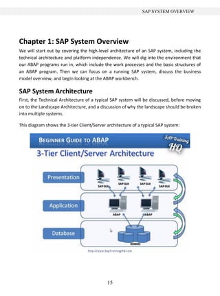
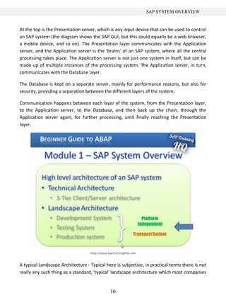
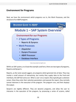
This document provides an overview of the SAP system architecture and environment for ABAP programs. It describes the typical 3-tier client/server architecture with presentation, application, and database layers. It also discusses the common landscape architecture with separate development, testing, and production systems. The environment for ABAP programs includes work processes that run programs on the application server independently of the operating system and database. The document introduces reports and dynpro programs that make up the main types of ABAP programs.

1. A-PDF Manual Split Demo. Purchase from www.A-PDF.com to remove the watermark

2. BEGINNER’S GUIDE
TO SAP ABAP
AN INTRODUCTION TO P ROGRAMMING SAP
APPLICATIONS USING ABAP
PETER M OXON
PUBLISHED BY:
SAPPROUK Limited
Copyright © 2012 by Peter Moxon. All rights reserved.
http://www.saptraininghq.com

3. Copyright, Legal Notice and Disclaimer:
All rights reserved.
No part of this publication may be copied, reproduced in any format, by any means,
electronic or otherwise, without prior consent from the copyright owner and
publisher of this book.
This publication is protected under the US Copyright Act of 1976 and all other
applicable international, federal, state and local laws, and all rights are reserved,
including resale rights: you are not allowed to give or sell this Guide to anyone else.
If you received this publication from anyone other than saptraininghq.com, you've
received a pirated copy. Please contact us via e-mail at support at saptraininghq.com
and notify us of the situation.
Although the author and publisher have made every reasonable attempt to achieve
complete accuracy of the content in this Guide, they assume no responsibility for
errors or omissions. Also, you should use this information as you see fit, and at your
own risk. Your particular situation may not be exactly suited to the examples
illustrated here; in fact, it's likely that they won't be the same, and you should adjust
your use of the information and recommendations accordingly.
This book is not affiliated with, sponsored by, or approved by SAP AG. Any
trademarks, service marks, product names or named features are assumed to be the
property of their respective owners, and are used only for reference. There is no
implied endorsement if we use one of these terms.
____________________________________________

4. Table of Contents
Contact the Author 12
Introduction 13
How to Use This Book 14
Chapter 1: SAP System Overview 15
SAP System Architecture 15
Environment for Programs 18
Work Processes 19
The Dispatcher 19
The Database Interface 20
First look at the ABAP Workbench 22
First Look 23
ABAP Dictionary 27
ABAP Editor 27
Function Builder 27
Menu Painter 28
Screen Painter 28
Object Navigator 28
Chapter 2: Data Dictionary 29
Introduction 29
Creating a Table 29
Creating Fields 33
Data Elements 34
Data Domains 36
Technical Settings 45
Entering Records into a Table 48
iv

5. Viewing the Data in a Table 51
Chapter 3 55
Creating a Program 55
Code Editor 57
Write Statements 62
Output Individual Fields 71
Chaining Statements Together 72
Copy Your Program 73
Declaring Variables 75
Constants 78
Chapter 4 79
Arithmetic – Addition 79
Arithmetic – Subtraction 80
Arithmetic – Division 81
Arithmetic – Multiplication 81
Conversion Rules 82
Division Variations 83
The standard form of division. 83
The integer form of division. 83
The remainder form of division. 84
Chapter 5 – Character Strings 85
Declaring C and N Fields 85
Data type C. 85
Data type N. 86
String Manipulation 87
Concatenate 87
v

6. Condense 88
NO-GAPS 89
Find the Length of a String 89
Replace 90
Search 90
SEARCH Example 1 91
SEARCH Example 2 91
SEARCH Example 3 92
SEARCH Example 4 92
Shift 93
Split 94
SubFields 96
Chapter 6 – Debugging Programs 98
Fields mode 102
System Variables 103
Table Mode 103
Breakpoints 105
Static Breakpoints 107
Watchpoints 108
Ending a Debug Session 111
Chapter 7: Working with Database Tables 113
Making a Copy of a Table 113
Add New Fields 116
Foreign Keys 117
Append Structures 122
Include Structures 124
vi

7. Key Fields 127
Deleting Fields 130
Deleting Tables 133
Chapter 8 – Working with Other Data Types 136
Date and Time Fields 136
Date Fields in Calculations 138
Time Fields in Calculations 141
Quantity and Currency Fields in Calculations 142
Chapter 9 – Modifying Data in a Database Table 146
Authorisations 146
Fundamentals 146
Database Lock Objects 148
Using Open SQL Statements 149
Using Open SQL Statements – 5 Statements 150
Insert Statement 151
Clear Statement 155
Update Statement 157
Modify Statement 158
Delete Statement 160
Chapter 10 – Program Flow Control and Logical Expressions 164
Control Structures 164
If Statement 164
Linking Logical Expressions Together 169
Nested If Statements 169
Case Statement 170
Select Loops 171
vii

8. Do Loops 172
Nested Do Loops 175
While Loops 178
Nested While Loops 179
Loop Termination – CONTINUE 180
Loop Termination – CHECK 181
Loop Termination – EXIT 182
Chapter 11 – Selection Screens 184
Events 184
Intro to Selection Screens 185
Creating Selection Screens 186
At Selection Screen 187
Parameters 188
DEFAULT 189
OBLIGATORY 190
Automatic Generation of Drop-Down fields 190
LOWER CASE 191
Check Boxes and Radio Button Parameters 192
Select-Options 193
Select-Option Example 196
Select-Option Additions 200
Text Elements 200
Variants 203
Text Symbols 209
Text Messages 211
Skip Lines and Underline 216
viii

9. Comments 218
Format a Line and Position 219
Element Blocks 221
Chapter 12 – Internal Tables 223
Introduction 223
Types of Internal Tables 224
Standard Tables 224
Sorted Tables 225
Hashed Table 225
Internal Tables - Best Practice Guidelines 225
Creating Standard and Sorted Tables 226
Create an Internal Table with Separate Work Area 227
Filling an Internal Table with Header Line 228
Move-Corresponding 232
Filling Internal Tables with a Work Area 234
Using Internal Tables One Line at a Time 235
Modify 236
Describe and Insert 236
Read 238
Delete Records 239
Sort Records 240
Work Area Differences 241
Loops 241
Modify 242
Insert 242
Read 242
ix

10. Delete 242
Delete a Table with a Header Line 243
CLEAR 243
REFRESH 243
FREE 243
Delete a Table with a Work Area 244
Chapter 13 – Modularizing Programs 245
Introduction 245
Includes 246
Procedures 249
Sub-Routines 250
Passing Tables 254
Passing Tables and Fields Together 255
Sub-Routines - External Programs 256
Function Modules 257
Function Modules – Components 258
Attributes Tab 262
Import Tab 262
Export Tab 263
Changing Tab 263
Tables Tab 263
Exceptions Tab 263
Source Code Tab 264
Function Module Testing 264
Function Modules - Coding 267
x

11. xi

12. Contact the Author
As the reader of this book you are my most important critic and commentator. I
would love to hear from you to let me know what you did and did not like about this
book, as well as to what you think I could do in future books to make them stronger.
E-mail: pete@sappro.co.uk
Please note that although I cannot personally help you learn SAP ABAP, I am
available for corporate hire for project management, technical lead and mentoring
programs.
Refer to my website http://www.saptraininghq.com to see all the training material I
have available and to get a good overview of my expertise.
12

13. INTRODUCTION
Introduction
This book has been written with SAP Super-User and Consultants in mind. Whether your
current job title is functional consultant, system support analyst, business consultant,
project manager for something entirely different, if you are responsible for all have an
interest in creating ABAP programs, then this book is for you.
Much of the book is written in the "How-To" style and will allow anybody to follow along
and create ABAP programs from scratch. It is written in such a way that each chapter
builds on the last so that you become familiar in lots of different aspects of SAP ABAP
programming to enable you to then start creating your own programs and understand
programs you will find in your own SAP system.
The principles and guidelines apply across all SAP modules whether you're writing
programs for HR, FI, SD or one of the many other modules within SAP.
Over my years of working with SAP systems I have had the great pleasure of working with
some top-notch functional and technical consultants who know how to document, plan
and develop SAP programs of all types. Likewise I have had the unpleasant experience of
working with lower quality consultants, who either race through or stumble and stutter
through their SAP work copying and pasting from one program or another resulting in
difficult to support programs. This ultimately often results in project delays and cost
overruns.
The aim of this book is to help you understand how SAP ABAP programs are put together
and developed so that you will produce detailed concise understandable and functional
programs that correspond with your specifications and most importantly delivered on
time and on budget.
13

14. INTRODUCTION
How to Use This Book
There are several ways to go through this book and the best way depends on your
situation.
If you are new to writing SAP programs then I suggest starting at the very beginning and
working through each chapter one after another.
If you are familiar with some SAP ABAP programming then you may want to use the table
of contents and jump to the chapter that interests you, but remember each chapter builds
on the previous chapter so some of the examples shown do require you to have
knowledge of the database tables we create in this book.
14

15. SAP SYSTEM OVERVIEW
Chapter 1: SAP System Overview
We will start out by covering the high-level architecture of an SAP system, including the
technical architecture and platform independence. We will dig into the environment that
our ABAP programs run in, which include the work processes and the basic structures of
an ABAP program. Then we can focus on a running SAP system, discuss the business
model overview, and begin looking at the ABAP workbench.
SAP System Architecture
First, the Technical Architecture of a typical SAP system will be discussed, before moving
on to the Landscape Architecture, and a discussion of why the landscape should be broken
into multiple systems.
This diagram shows the 3-tier Client/Server architecture of a typical SAP system:
15

16. SAP SYSTEM OVERVIEW
At the top is the Presentation server, which is any input device that can be used to control
an SAP system (the diagram shows the SAP GUI, but this could equally be a web browser,
a mobile device, and so on). The Presentation layer communicates with the Application
server, and the Application server is the 'brains' of an SAP system, where all the central
processing takes place. The Application server is not just one system in itself, but can be
made up of multiple instances of the processing system. The Application server, in turn,
communicates with the Database layer.
The Database is kept on a separate server, mainly for performance reasons, but also for
security, providing a separation between the different layers of the system.
Communication happens between each layer of the system, from the Presentation layer,
to the Application server, to the Database, and then back up the chain, through the
Application server again, for further processing, until finally reaching the Presentation
layer.
A typical Landscape Architecture - Typical here is subjective, in practical terms there is not
really any such thing as a standard, 'typical' landscape architecture which most companies
16

17. SAP SYSTEM OVERVIEW
use. However, it is common to find a Development system, a Testing system and a
Production system:
The reason for this is fairly simple. All the initial development and testing is done on a
Development system, which ensures other systems are not affected. Once developments
are at a stage where they may be ready to be tested by an external source, or someone
within the company whose role is to carry out testing, the developments are moved, using
what is called a Transport System, to the next system (here, the Testing system).
Normally, no development at all is done on the testing system; it is just used for testing
the developments from the development system. If everything passes through the Testing
system, a Transport system is used again to move the developments into the Production
environment. When code enters the Production environment, this is the stage at which it
is turned on, and used within the business itself.
The landscape architecture is not separated just for development purposes; the company
may have other reasons. This could be the quantity of data in the Production system,
which may be too great to be used in the development environment (normally the
Development and Testing systems are not as large as the Production system, only needing
a subset of data to test on). Also, it could be for security reasons. More often than not,
companies do not want developers to see live production data, for data security reasons
(for example, the system could include employee data or sales data, which a company
would not want people not employed in those areas to see). Normally, then, the
Development and Testing systems would have their own set of data to work with.
The three systems described here, normally, are a minimum. It can increase to four
systems, perhaps with the addition of a Training system, or perhaps multiple projects are
running simultaneously, meaning there may be two separate Development systems, or
Testing systems, even perhaps a Consolidation system before anything is passed to the
Production environment. This is all, of course, dependent on the company, but commonly
each system within the Landscape architecture will have its own Application server and its
own Database server, ensuring platform independence.
17

18. SAP SYSTEM OVERVIEW
Environment for Programs
Next, we have the environment which programs run in, the Work Processes, and the
structure of an ABAP program.
Within an SAP system, or at least the example used here, there are two types of programs,
Reports and Dynpro’s.
Reports, as the name would suggest, are programs which generate lists of data. They may
involve a small amount of interactivity, but mainly they supply data to the front-end
interfaces, the SAP GUI and so on. When a user runs a report, they typically get a selection
screen. Once they enter their selection parameters and execute the report, they normally
cannot intervene in the execution of the program. The program runs, and then displays
the output.
Dynpro’s are slightly different. They are dynamic programs, and allow the user to
intervene in the execution of the program, by processing a series of screens, called
18

19. SAP SYSTEM OVERVIEW
Dialogue screens. The user determines the flow of the program itself by choosing which
buttons or fields to interact with on the screen. Their action then triggers different
functions which have been coded within the flow logic of the program. While reports are
being created, interfaces are also to be generated which are classed as Dynpro’s, for all
the selection criteria.
Most of the work done by people involved with ABAP is done within Report programs, and
even though these programs are labelled 'Reports', they do not always generate output.
The Report programs are there to process the logic, reading and writing to the Database,
in order to make the system work.
Work Processes
Every program that runs in an SAP system runs on what are called Work Processes, which
run on the Application server. Work Processes themselves work independently of the
computer's operating system and the Database that it interacts with, giving the
independence discussed earlier with regard to the Technical architecture. When an SAP
system is initially set up, the basis consultants (who install the system, keep it running,
manage all the memory and so on) configure SAP in such a way that it automatically sets
the number of Work Processes programs use when they start, the equivalent of setting up
a pre-defined number of channels or connections to the Database system itself, each of
which tend to have their own set of properties and functions.
The Dispatcher
You might come across something referred to as the Dispatcher. The SAP system has no
technical limits as to the number of users who can log on and use it, generally the number
of users who can access an SAP system is much larger than the number of available Work
Processes the system is configured for. This is because not everybody is sending
instructions to the Application server at exactly the same time. Because of this, users
cannot be assigned a certain number of processes while they are logged on.
The Dispatcher controls the distribution of the Work Processes to the system users. The
Dispatcher keeps an eye on how many Work Processes are available, and when a user
triggers a transaction, the Dispatcher's job is to provide that user with a Work Process to
use. The Dispatcher tries to optimise things as far as possible, so that the same Work
Process receives the sequential Dialogue steps of an application. If this is not possible, for
example because the user takes a long time between clicking different aspects of the
19

20. SAP SYSTEM OVERVIEW
screen, it will then select a different Work Process to continue the processing of the
Dialogue program. It is the Work Process which executes an application, and it is the Work
Process which has access to the memory areas that contain all of the data and objects an
application uses. It also makes three very important elements available.
The first is the Dynpro processor. All Dynpro programs have flow and processing logic, and
it is the Dynpro processor's job to handle the flow logic. It responds to the user's
interactions, and controls the further flow of the program depending on these
interactions. It is responsible for Dialogue control and the screen itself, but it is important
to remember that it cannot perform calculations; it is purely there to manage the flow
logic of a program.
The next important element is the ABAP processor, which is responsible for the processing
logic of the programs. It receives screen entries from the Dynpro processor, and transmits
the screen output to the program. It is the ABAP processor which can perform the logical
operations and arithmetical calculations in the programs. It can check authorisations, and
read and write to the Database, over the Database Interface.
The Database Interface
The Database Interface is the third important element. It is a set of ABAP statements that
are Database independent. What this means is that a set of ABAP statements can be used
that, in turn, can communicate with any type of Database that has been installed when
the system was set up. Whether this is, for example, a Microsoft SQL server or an Oracle
Database, you can use the same ABAP statements, called Open SQL, to control the entire
Database reading and writing over the Database Interface. The great advantage of this is
that the ABAP statements have encapsulation, meaning the programmers do not need to
know which physical Database system the ABAP system they are using actually supports.
There are times when you may want to use a specific SQL statement native to the
database which is installed. ABAP is designed in such a way that if this type of coding is
necessary, this facility is available. It is possible to directly access the Database through
the programs using native SQL statements, but this is not encouraged. Normally, when
systems are set up, the system administrator will forbid these practices, due to the
security and stability risks to the system which may be introduced. If you are going to be
programming ABAP, make sure Open SQL is used, because then anyone subsequently
looking at the programs will understand what is trying to be achieved.
20

21. SAP SYSTEM OVERVIEW
21

22. SAP SYSTEM OVERVIEW
First look at the ABAP Workbench
It is now time to take a first look at an SAP ABAP program. The following section will look
at the SAP System and introduce the ABAP Workbench. But before doing so, let's take a
look at the structure of an ABAP program.
Like many other programming languages, ABAP programs are normally structured into
two parts.
The first is what is considered to be the Declaration section. This is where you define the
data types, structures, tables, work area variables and the individual fields to be used
inside the programs. This is also where you would declare global variables that will be
available throughout the individual subsections of the program. When creating an ABAP
program, you do not only declare global variables, but you also have the option to declare
22

23. SAP SYSTEM OVERVIEW
variables that are only valid within specific sections inside the programs. These sections
are commonly referred to as internal Processing Blocks.
The Declaration part of the program is where you define the parameters used for the
selection screens for the reports. Once you have declared tables, global variables and data
types in the Declaration section of the program, then comes the second part of the ABAP
program, where all of the logic for the program will be written. This part of an ABAP
program is often split up into what are called Processing Blocks.
The Processing Blocks defined within programs can be called from the Dynpro processor,
which were discussed previously, depending on the specific rules created within the
program. These Processing Blocks are almost always just small sections of programming
logic which allow the code to be encapsulated.
First Look
When logged into an SAP system it will look something similar to the image below.
The way the SAP GUI looks may vary, the menu to the side may be different, but here the
display show a minimal menu tree which will be used throughout this book.
The first thing to do here is look at the ABAP Workbench. To access this, you use the menu
on the left hand side. Open the SAP menu, choose Tools and open the ABAP Workbench,
where there will be four different options.
23

24. SAP SYSTEM OVERVIEW
The first thing to look at is a quick overview of how to run a transaction in SAP. There are
two ways to do this. Firstly, if the overview folder is opened, any item which does not look
like a folder itself, is a transaction which can be run. In this instance, we can see the Object
Navigator:
Double click this, and the transaction will open:
24

25. SAP SYSTEM OVERVIEW
To exit out of the transaction, click the Back button:
The second way of running a transaction is to enter the transaction code into the
transaction code input area:
A useful tip to become familiar with the names of transactions is to look at the Extras
menu --> open Settings and in the dialogue box which appears, select the option 'Display
technical names' and click the 'Continue' icon:
25

26. SAP SYSTEM OVERVIEW
The menu tree will be refreshed, and when the 'Overview' folder is opened, the
transaction codes will be made visible. It is now possible to become familiar with them,
and enter them directly into the transaction code input area:
Now, a step-by-step look will be taken through the major transactions of the ABAP
Workbench to become familiar with, and use, as an ABAP developer.
26

27. SAP SYSTEM OVERVIEW
ABAP Dictionary
One thing most programs will have in common is that they will read and write data to and
from the Database tables within the SAP system. The ABAP Workbench has a transaction
to allow the creation of Database tables, view the fields which make up these tables and
browse the data inside. This is called the ABAP Dictionary. The ABAP Dictionary can be
found by expanding the ABAP Workbench menu tree --> 'Development'. The transaction
code to run the ABAP dictionary directly is SE11:
ABAP Editor
The next and probably most commonly used part of the ABAP Workbench is the ABAP
Editor, which much of this course will focus upon. The ABAP Editor is where all of the code
is created, the logic built and, by using forward navigation (a function within an SAP
system which will be discussed later), function modules defined, screens created and so
on. The ABAP Editor can be found under the 'Development' menu, as shown above and
with transaction code SE38.
Function Builder
The next important part of the Workbench is the Function Builder, which is similar to the
ABAP Editor. Its main function is to define specific tasks that can be called from any other
program. Interfaces are created in the Function Builder, where the different data
elements and different types of tables are defined, that can be passed to and from the
Function which is built. The Function Builder will be discussed a little later on, when the
programs created are encapsulated into function modules. The Function Builder can be
27

28. SAP SYSTEM OVERVIEW
called with transaction code SE37.
Menu Painter
The next item to look at here is called the Menu Painter, which can be found in the 'User
Interface' folder inside the 'Development' menu, or with transaction code SE41. This is a
tool which can be used to generate menu options, buttons, icons, menu bars, transaction
input fields, all of which can trigger events within the program. You can define whether
events are triggered using a mouse click, or with a keyboard-based shortcut. For example,
in the top menu bar here, the 'Log off' button can be seen, which can be triggered by using
(Shift + F3):
Screen Painter
While the Menu Painter is used for building menu items, menu bars and so on, the next
item on the list is the Screen Painter, transaction code SE51, which allows you to define
the user input screen, meaning that you can define text boxes, drop-down menus, list
boxes, input fields, tabbed areas of the screen and so on. It allows you to define the whole
interface which the user will eventually use, and behind the initial elements that are put
on the screen, you can also define the individual functions which are called when the user
interacts with them.
Object Navigator
The last item to look at here is the Object Navigator, a tool which brings together all the
previous tools, providing a highly efficient environment in which to develop programs.
When building large programs, with many function modules, many screens, the Object
Navigator is the ideal tool to use to navigate around the development. It can be found in
the 'Overview' menu of the ABAP Workbench, with transaction code SE80.
These are the main features of the ABAP Workbench interacted with during this course. In
the SAP menu tree, there are evidently many more transactions which can be used to help
develop programs, but these cover the vast majority of development tools which will be
used.
28

29. DATA DICTIONARY
Chapter 2: Data Dictionary
Introduction
This chapter will focus specifically on the Data Dictionary. This is the main tool used to
look at, understand and enhance the Database and Database tables which are used by the
SAP system. You can view standard tables delivered by SAP using this tool, create new
tables and enhance the existing tables delivered by SAP with new fields. There are many
other features involved in the Data Dictionary, but the focus here will be on the basic ones
so as to build on this later on when creating ABAP programs.
First, a database table will be created, involving the creation of fields, data elements and
domains. An explanation of what each of these is, and why they are necessary to the
tables built will be given. During the building of the tables, the tools used to check for
errors will be shown. Once these errors are eradicated, the tables can be activated so that
they can be used within the system.
After this, a look will be taken at maintaining the technical settings of the table created,
which will allow the entry of data, before finally looking at the data which has been
entered using standard SAP transactions available in the SAP system.
Creating a Table
With the SAP GUI open, you will be able find the Data Dictionary in the SAP menu tree.
This is done via the Tools menu. Open the ABAP Workbench and click the 'Development'
folder, where the ABAP Dictionary can be found and double-clicked. Alternatively, use the
transaction code SE11:
Now, the initial screen of the ABAP Dictionary will appear:
29

30. DATA DICTIONARY
To create a table, select the 'Database table' option. In this exercise a transparent table
will be created. Other types of table do exist (such a cluster tables and pool tables), but at
this early stage the transparent table variety is the important one to focus upon.
The table name must adhere to the customer-defined name space, meaning that the
name must begin with the letter Z or Y, most commonly this will be Z. In this example, the
table will show a list of employees within a company, so, in the 'Database table' area, type
'ZEMPLOYEES' and click the 'Create' button.
Once this is done, a new screen will appear:
30

31. DATA DICTIONARY
In the 'Short text' field, a description for the table must be included, enter 'Employees':
In the 'Delivery and Maintenance' tab (which opens by default), look at the 'Delivery class'
section, select the field and then click the drop-down button, where a list of Delivery
classes will be shown and selected:
31

32. DATA DICTIONARY
For the table being created here, choose 'Application table', as the data held in the table
fits the description 'master and transaction data'.
In the field below this, labelled 'Data Browser/Table View Maint.', choose the
'Display/Maintenance allowed' option, which will allow for data entry directly into the
table later on. It should look like this:
Before going any further, click the 'Save' button:
A window appears titled 'Create Object Directory Entry'.
Nearly all development work done with SAP is usually done within a development
environment, before being moved on to, for example, a quality assurance environment
and on further to production. This window allows you to choose the appropriate
Development class which is supported by other systems where the work may be moved
on to. In this example scenario, though, developments will not be moved on to another
system, so click 'Local object', so as to indicate to the system (via the phrase '$TMP' which
appears) that the object is only to exist within the development system and not to be
transported elsewhere. Once this is done, the status bar at the bottom will show that the
object has been saved:
32

33. DATA DICTIONARY
To check everything has worked as we want, select the 'Go to' menu and selects the
'Object directory entry' option, a similar pop-up box to the previous one will appear,
where the 'Development class' field will show '$TMP', confirming this has been done
correctly.
Creating Fields
The next step is to begin creating Field names for the table, in the 'Fields' tab:
Fields, unlike the name of the table, can begin with any letter of the alphabet, not just Z
and Y and can contain up to 16 characters.
33

34. DATA DICTIONARY
Tables must include at least one Key field, which is used later for the searching and sorting
of data, and to identify each record as being unique.
An Initial value can be assigned to each field, for example, in the case of a field called
Employee Class you could say the majority of employees are Regular Staff ('S'), but some
are Directors, with a code of 'D'. The standard initial value would be 'S', but the user could
change some of these to a 'D' later on.
Data Elements
Every Field in the table is made up of what is called a Data Element, which defines specific
attributes of each field.
The first Field to be created here is an important one within an SAP system, and identifies
the client which the records are associated with. In the Field name, enter 'Client', and in
the Data Element, type 'MANDT'. This Data Element already exists in the system, and after
entering it, the system automatically fills in the Data Type, the Length, Number of
Decimals and Short text for the Data Element itself. Ensure that the 'Client' field is made a
Key field in the table by checking the 'Key' box.
The next field will be called 'Employee'. Again, check the box to make this a Key field, and
enter the new Data Element 'ZEENUM' (Data Elements broadly must adhere to the
customer name space by beginning with Z or Y). Once this is done, click the save button.
Next, because the Data Element 'ZEENUM' does not yet exist, it must be created. If you try
to activate or even check the table (via the 'Check' button), an error message is
displayed:
Until the Data Element 'ZEENUM' is created, it cannot be used within the system. To do
this, forward navigation is used. Double-click the new Data Element, and a window
labelled 'Create Data element' appears. Answer 'Yes' to this, and the 'Maintain Data
Element' window comes up.
34

35. DATA DICTIONARY
35

36. DATA DICTIONARY
In the 'Short text' area, enter 'Employee Data Element'. Next, the Elementary data type,
called the 'Domain', must be defined for the new Data element. Domains must adhere to
the customer name space, so in this instance the same name as the Data element will be
given: 'ZEENUM', (though giving both the same name is not imperative). Again, forward
navigation will be used to create the Domain.
Data Domains
Double-click the entry ('ZEENUM') in the Domain area, and agree to save the changes
made. Now, the 'Create Object Directory Entry' window will re-appear and again it is
important to save this development to the '$TMP' development class, via the 'save' or
'local object' button visible in this window.
After doing this, a window will appear stating that the new Domain 'ZEENUM' does not
exist. Choose 'Yes' to create the Domain, and in the window which appears, type into the
'Short text' box a description of the Domain. In this example, 'Employee Domain':
36

37. DATA DICTIONARY
The 'Definition' tab, which, as shown above, opens automatically. The first available field
here is 'Data type', click inside the box and select the drop-down menu, and a number of
generic data types already existing within the ABAP dictionary will appear.
The 'NUMC' type is the one to be used here for the Employee data, a “character string
with only digits”. Once this selection is double-clicked, it will appear in the 'Data type' area
in the 'Definition' tab.
Next, in the 'No. characters' field, enter the number 8, indicating that the field will contain
a maximum of 8 characters, and in the 'Decimal places' area, enter 0. An Output length of
8 should be selected, and then press Enter.
The 'NUMC' field's description should re-appear, confirming that this is a valid entry.
Next, select the 'Value range' tab, which is visible next to the 'Definition' tab just used:
This is where you set valid value ranges for the Domain created. Once this is set, any
subsequent user entering values outside the valid value range will be shown an error
37

38. DATA DICTIONARY
message and be requested to enter a valid entry. Here, there are three options.
First, where you can see 'Single values', it is possible to enter a list of individual
valid values which can be entered by the user.
Second, 'Intervals', where you can enter a lower and upper limit for valid values,
for example 1 and 9, which saves the effort of entering 9 individual single values in
the 'Single values' section.
Last, the 'Value table' box visible at the bottom. When there are a large number of
possible entries, this is a common method (to do this you must specify a complete
valid value table entry list, in which case it is also necessary to introduce foreign
keys to the table, to ensure the user's entries are tested against the value stored
in the value table created).
This example Domain, however, does not require any Value range entry, so just click the
save button and, again, assign it as a 'Local object'.
The next step is to Activate the object, allowing other Data elements to use this domain
going forward. In the toolbar click the small matchstick icon (also accessible by pressing
CTRL +F3).
A pop-up window appears, listing the 3 currently inactive objects:
It may be possible to activate all of the objects together, but this is not advised. In a typical
development environment, a number of people will be creating developments
simultaneously, and quite often, others' objects will appear in this list.
At this point, it is only the Domain which is to be activated, the top entry labelled 'DOMA',
with the name 'ZEENUM'. When this is highlighted, click the green tick continue button.
The window should disappear, and the status bar will display the message 'Object(s)
38

39. DATA DICTIONARY
activated'
Now it is possible to proceed with the creation of the table. Forward navigation was used
for generating the Domain, so click the 'Back' button, or press F3 to return to the
'Maintain Data Element' screen. As the domain is active, the description entered
previously should appear by the area where 'ZEENUM' was typed, along with other
Domain properties which have been created:
Next, the Field labels must be created, so click that tab. The Field labels entered here will
appear as field labels in the final table. In this example they should read 'Employee', or
better, 'Employee Number'. If this does not fit within the area given, just tailor it so that it
still makes sense, for example typing 'Employee N' into the 'Short' Field label box. Once
the text has been put into the Field label spaces, press enter, and the 'Length' section will
automatically be filled in:
39

40. DATA DICTIONARY
Once this is complete, Save and Activate the element via the toolbar at the top. The
inactive objects window will reappear, where two inactive objects will remain. Highlight
the Data element (labelled 'DTEL') and click the green tick
Continue button at the bottom.
Again, the status bar should display 'Object(s) activated'.
Press the back button to return to the Table maintenance screen. Here you will now see
that the 'EMPLOYEE' column has the correct Data Type, Length, Decimals and Short text,
thus indicating the successful creation of a Data element and Domain being used for this
Field.
Next, the same practices will be used to create four additional fields.
The next field to create should be titled 'SURNAME'. This time it should not be selected as
a Key field, so do not check the box. The Data element, in this instance, is labelled
'ZSURNAME':
Now, forward navigation will again be used. Double-click ‘ZSURNAME’; choose 'Yes' to
save the table and 'Yes' again to create the new Data element. The 'Maintain Data
Element' window will appear which will be familiar from the previous steps.
In the 'Short text' box this time type 'Surname Data Element' and title the new domain
40

41. DATA DICTIONARY
'ZSURNAME':
Double-click the new domain and save the Data element, assigning it a 'Local object' and
then choose 'Yes' to create the new Domain.
The Domain maintenance screen will reappear. Enter the short text 'Surname' and, this
time; the Data type to select is 'CHAR', a Character string.
The number of characters and output length should both be set to 40, then press enter to
be sure everything has worked, and click the Activate button.
41

42. DATA DICTIONARY
Note that the Save button has not been pressed this time, as the Activate button will also
save the work automatically. Ensure you assign the object to the $TMP development class
as usual.
In the Activate menu, select the object (the domain (labelled 'DOMA') named
'ZSURNAME') to be activated, and click the green tick continue button. The status bar
should read 'Object saved and activated'.
Following this, click Back or F3 to return to the Maintain Data element screen. Ensure the
domain attributes have appeared (Short text, Data type, Length and so on). In the Field
Label tab, enter 'Surname' in each box and press Enter to automatically fill the 'Length'
boxes and then activate the Data element (in the Activate menu, the 'DTEL' object named
'ZSURNAMES'), checking the status bar to ensure this has occurred with any errors:
Again, press Back to return to the Maintain Table screen, where the new Data element will
be visible:
42

43. DATA DICTIONARY
The next field to be created is titled 'FORENAME', and the data element 'ZFORENAME'.
Click to create the Data element and follow the steps above again.
In the Maintain Data Element screen, the Short text should read 'Forename Data Element'
and the domain 'ZFORENAME'. Save this and choose 'Yes' to create the domain.
The domain's short text should read 'Forename'. Use the CHAR data type again and a
Length and Output length of 40. Next, Activate the Domain as before.
Return to the Maintain Data Element screen. Type 'Forename' into the four Field label
boxes. Press enter to fill the length boxes and then Activate the Data Element named
'ZFORENAME' as before. Go back again to see the table:
43

44. DATA DICTIONARY
The next field will be called 'Title' and the Data Element 'ZTITLE', follow the steps above
again to create this field with the following information:
The Data element short text should read 'Title Data Element' and the domain should be
named 'ZTITLE'.
The Domain Short text should be 'Title' and the Data type is again 'CHAR'. This time the
Length and Output length will be 15.
The Field labels should all read 'Title'.
Activate all of these and go back to view the new, fifth field in the Table.
The final field which will be created for this table is for Date of Birth. In the Field box type
'DOB' and create the Data element 'ZDOB' using the steps from the previous section and
this information:
The Data element short text should read 'Date of Birth Data Element' and the domain
should be named 'ZDOB'.
The Domain Short text should be 'Date of Birth' and the Data type is, this time, 'DATS',
after which an information box will appear to confirm this. Click the green tick to continue:
44

45. DATA DICTIONARY
For the DATS data type, the Length and Output lengths are set automatically at 8 and 10
(the Output length is longer as it will automatically output dividers between the day,
month and year parts of the date).
The Field labels should all read 'Date of Birth', except the 'Short' label where this will not
fit, so just type 'DOB' here. Activate the Domain and Data element, and return to the
table.
Technical Settings
Once this has been saved, the next step is to move on to maintaining the technical settings
of the Table. Before creating the final Database table, SAP will need some more
information about the table being created.
Select 'Technical settings' via the toolbar above the table, through the 'Go to' menu, or
45

46. DATA DICTIONARY
with the shortcut CTRL+SHIFT+F9.
Here, it is important to tell the system what Data class is to be used, so select the drop
down button. There are five different options, with accompanying descriptions. For this
table, select the first, labelled 'APPL0', and double-click it:
For the 'Size category' field, again click the drop-down button. Here, you have to make an
estimate as to the amount of data records which will be held within the table so that the
system has some idea of how to create the tables in the underlying database. In this
instance, it will be a relatively small amount of information, so select the first size
category, labelled 0:
46

47. DATA DICTIONARY
Below this are the Buffering options. Here, 'Buffering not allowed' should be selected:
This prevents the table contents from being loaded into memory for reading, stopping the
table from being read in advance of the selection of the records in the program. You may,
correctly, point out that it may be advantageous to hold the table in the memory for
speed efficiency, but in this example, this is not necessary. If speed was an issue in a
development, buffering would then be switched on, ensuring the data is read into
memory. In the case of large tables which are accessed regularly but updated
infrequently, this is the option to choose.
Nothing else on the 'Maintain Technical Settings' screen needs to be filled at this point, so
click Save and then go back to the table itself. If all of this is successful, then the table
should now be in a position to be activated and the entry of records can begin. Click the
Activate icon to activate the table and check the status bar, which should again read
'Object Activated'.
47

48. DATA DICTIONARY
Entering Records into a Table
Now that the table has been created, data can be entered. To do this, enter the 'Utilities'
menu, scroll to 'Table contents', and then 'Create Entries':
A Data-entry screen will appear which has automatically been generated from the table
created. The field names correspond here to the technical names given when we created
them. To change these to the Field labels which we set up, enter the 'Settings' menu and
select 'User Parameters'. This facility allows you to tailor how tables look for your own
specific user ID. Select the 'Field label' radio button and click 'Continue':
48

49. DATA DICTIONARY
The Field labels created will now appear as they were defined when creating the table:
The Employee Number field is limited to 8 characters, and the data type was set to NUMC,
so only numerical characters can be entered. Create a record with the following data:
Employee Number: '10000001'
Surname: 'Brown'
Forename: 'Stephen'
Title: 'Mr'
Date of Birth: '16.02.1980':
Press Enter and the system will automatically put the names in upper case, and validate
each field to ensure the correct values were entered:
49

50. DATA DICTIONARY
Click Save and the status bar should state 'Database record successfully created'. Next,
click the 'Reset' button above the data entry fields to clear the fields for the next entry.
Create another record with the following data:
Employee Number '10000002'
Surname 'Jones'
Forename 'Amy'
Title 'Mrs'
Date of Birth '181169'.
Note that this time the Date of Birth has been filled in without the appropriate dividers.
When Enter is pressed, the system automatically validates all fields, correcting the Date of
Birth field to the correct formatting itself:
50

51. DATA DICTIONARY
Save, Reset, and then further records can be entered following the same steps:
Note that if dates are entered in the wrong format, an error message will appear in the
status bar:
Viewing the Data in a Table
Now that data has been entered into the table, the final few steps will allow this data to
be viewed.
Having entered several data records in the manner discussed previously, click the Back key
to return to the 'Dictionary: Display Table' screen. To view the table created with the data
entered, from the 'Utilities' menu, select 'Table contents' and then 'Display':
51

52. DATA DICTIONARY
A selection screen will then appear, allowing you to enter or choose filter values for the
fields you created. The selection screen is very useful when you have lots of data in your
table. In this case, though, only five records have been entered, so this is unnecessary.
However, for example if you were to only want to focus on a single employee number, or
a small range, these figures can be selected from this screen:
To view all of the records, do not enter any data here. Just click the 'Execute' button,
which is displayed in the top left corner of the image above, or use the shortcut F8. You
will now see a screen showing the data records you entered in the previous section:
52

53. DATA DICTIONARY
If further fields were to exist, the screen would scroll further to the right, meaning not all
fields could be displayed simultaneously due to field size properties.
If you want to see all of the data for one record, double-click on the record and this will be
shown. Alternatively, several records can be scrolled through by selecting the desired
records via the check-boxes to the left of the 'Client' column and then clicking the 'Choose'
icon on the toolbar:
These can then be individually viewed and scrolled through with the 'Next entry' button:
To return to the full table then, simply click the Back button, or press F3.
Experiment with the table created, using the toolbar's range of options to filter and sort
the information in a number of ways:
53

54. DATA DICTIONARY
For example, to organise alphabetically by forename, click to select the 'Forename' field,
and then click the 'Sort ascending' button:
There are a number of things which can be achieved in this table view, and it can be a
useful tool for checking the data within an SAP system without going through the
transaction screens themselves.
54

55. YOUR FIRST ABAP PROGRAM
Chapter 3
Creating a Program
To begin creating a program, access the ABAP Editor either via transaction code SE38, or
by navigating the SAP menu tree to Tools  ABAP Workbench  Development, in which
the ABAP Editor is found. Double-click to execute.
A note to begin: it is advisable to keep the programs created as simple as possible. Do not
make them any more complicated than is necessary. This way, when a program is passed
on to another developer to work with, fix bugs and so on, it will be far easier for them to
understand. Add as many comments as possible to the code, to make it simpler for
anyone who comes to it later to understand what a program is doing, and the flow of the
logic as it is executed.
The program name must adhere to the customer naming conventions, meaning that here
it must begin with the letter Z. In continuation of the example from the previous chapter,
in this instance the program will be titled ‘Z_Employee_List_01’, which should be typed
into the ‘Program’ field on the initial screen of the ABAP Editor. Ensure that the ‘Source
code’ button is checked, and then click ‘Create’:
55

56. YOUR FIRST ABAP PROGRAM
A ‘Program Attributes’ window will then appear. In the ‘Title’ box, type a description of
what the program will do. In this example, “My Employee List Report”. The Original
language should be set to EN, English by default, just check this, as it can have an effect on
the text entries displayed within certain programs. Any text entries created within the
program are language-specific, and can be maintained for each country using a translation
tool. This will not be examined at length here, but is something to bear in mind.
In the ‘Attributes’ section of the window, for the ‘Type’, click the drop-down menu and
select ‘Executable program’, meaning that the program can be executed without the use
of a transaction code, and also that it can be run as a background job. The ‘Status’ selected
should be ‘Test program’, and the ‘Application’ should be ‘Basis’. These two options help
to manage the program within the SAP system itself, describing what the program will be
used for, and also the program development status.
For now, the other fields below these should be left empty. Particularly ensure that the
‘Editor Lock’ box is left clear (selection of this will prevent the program from being edited).
‘Unicode checks active’ should be selected, as should ‘Fixed point arithmetic’ (without
this, any packed-decimal fields in the program will be rounded to whole numbers). Leave
the ‘Start using variant’ box blank. Then, click the Save button.
56

57. YOUR FIRST ABAP PROGRAM
The familiar ‘Create Object Directory Entry’ box from the previous section should appear
now, click the ‘Local object’ option as before to assign the program to the temporary
development class. Once this is achieved, the coding screen is reached.
Code Editor
Here, focus will be put on the coding area. The first set of lines visible here are comment
lines. These seven lines can be used to begin commenting the program. In ABAP,
comments can appear in two ways. Firstly, if a * is placed at the beginning of a line, it
turns everything to its right into a comment.
57

58. YOUR FIRST ABAP PROGRAM
Note that the * must be in the first column on the left. If it appears in the second column
or beyond, the text will cease to be a comment.
A comment can also be written within a line itself, by using a “. Where this is used,
everything to the right again becomes a comment. This means that it is possible to add
comments to each line of a program, or at least a few lines of comments for each section.
The next line of code, visible above, begins with the word REPORT. This is called a
STATEMENT, and the REPORT statement will always be the first line of any executable
program created. The statement is followed by the program name which was created
previously. The line is then terminated with a full stop (visible to the left of the comment).
Every statement in ABAP must be followed by a full stop, or period. This allows the
statement to take up as many lines in the editor as it needs, so for example, the REPORT
statement here could look like this:
58

59. YOUR FIRST ABAP PROGRAM
As long as the period appears at the end of the statement, no problems will arise. It is this
period which marks where the statement finishes.
If you require help with a statement, place the cursor within the statement and choose
the ‘Help on...’ button in the top toolbar:
A window will appear with the ABAP keyword automatically filled in. Click the continue
button and the system will display help on that particular statement, giving an explanation
of what it is used for and the syntax. This can be used for every ABAP statement within an
SAP system. Alternatively, this can be achieved by clicking the cursor within the
statement, and pressing the F1 key:
59

60. YOUR FIRST ABAP PROGRAM
A further tip in this vein is to use the ‘ABAP Documentation and Examples’ page, which
can be accessed by entering transaction code ABAPDOCU into the transaction code field.
The menu tree to the left hand side on this screen allows you to view example code, which
one’s own code can later be based upon. This can either be copied and pasted into the
ABAP editor, or experimented with inside the screen itself using the Execute button to run
the example code:
60

61. YOUR FIRST ABAP PROGRAM
Returning to the ABAP editor now, the first line of code will be written. On the line below
the REPORT statement, type the statement: write ‘HELLO SAP WORLD’.
The write statement will, as you might expect, write whatever is in quotes after it to the
output window (there are a number of additions which can be made to the write
statement to help format the text, which we will return in a later chapter).
Save the program, and check the syntax with the ‘Check’ button in the toolbar (or via CTRL
+ F2). The status bar should display a message reading “Program Z_EMPLOYEE_LIST_01 is
syntactically correct”. Then, click the ‘Activate’ button, which should add the word ‘Active’
next to the program name. Once this is done, click the ‘Direct processing’ button to test
the code:
61

62. YOUR FIRST ABAP PROGRAM
The report title and the text output should appear like this, completing the program:
Write Statements
Now that the first program has been created, it can be expanded with the addition of
further ABAP statements. Use the Back button to return from the test screen to the ABAP
editor.
Here, the tables which were created in the ABAP Dictionary during the first stage will be
accessed. The first step toward doing this is to include a table’s statement in the program,
which will be placed below the REPORT statement. Following this, the table name which
62

63. YOUR FIRST ABAP PROGRAM
was created is typed in, z_employee_list_01, and, as always, a period to end the
statement:
While not essential, to keep the format of the code uniform, the Pretty Printer facility can
be used. Click the ‘Pretty Printer’ button in the toolbar to automatically alter the text in
line with the Pretty Printer settings (which can be accessed through the Utilities menu,
Settings, and the Pretty Printer tab in the ABAP Editor section):
Once these settings have been applied, the code will look slightly tidier, like this:
63

64. YOUR FIRST ABAP PROGRAM
Let us now return to the TABLES statement. When the program is executed, the TABLES
statement will create a table structure in memory based on the structure previously
defined in the ABAP Dictionary. This table structure will include all of the fields previously
created, allowing the records from the table to be read and stored in a temporary
structure for the program to use.
To retrieve from our data dictionary table and place them into the table structure, the
SELECT statement will be used.
Type SELECT * from z_employee_list_01. This is telling the system to select everything
(the * refers to all-fields) from the table. Because the SELECT statement is a loop, the
system must be told where the loop ends. This is done by typing the statement
ENDSELECT. Now we have created a select loop let’s do something with the data we have
are looping through. Here, the WRITE command will be used again. Replace the “write
‘HELLO SAP WORLD’.” line with “write z_employee_list_01.” to write every row of the
table to the output window:
Check the code with the ‘Check’ button, and it will state that there is a syntax error:
64

65. YOUR FIRST ABAP PROGRAM
The cursor will have moved to the TABLES statement which was identified, along with the
above warning. The name “Z_EMPLOYEE_LIST_01” appears to be incorrect. To check this,
open a new session via the New Session button in the toolbar . Execute the ABAP
Dictionary with transaction code SE11, search for Z* in the ‘Database table’ box and it will
bring back the table ZEMPLOYEES, meaning that the initial table name
Z_EMPLOYEE_LIST_01 was wrong. Close the new session and the syntax error window and
type in the correct table name ‘ZEMPLOYEES’ after the TABLES state. Your screen should
look like this:
Save the program and check the code, ensuring the syntax error has been removed, and
then click the Test button (F8) and the output window should display every row of the
table:
65

66. YOUR FIRST ABAP PROGRAM
Look at the data in the output window. The system has automatically put each line from
the table on a new row. The WRITE statement in the program did not know that each row
was to be output on a new line; this was forced by some of the default settings within the
system regarding screen settings, making the line length correspond to the width of the
screen. If you try to print the report, it could be that there are too many columns or
characters to fit on a standard sheet of A4. With this in mind, it is advisable to use an
addition to the REPORT statement regarding the width of each line.
Return to the program, click the REPORT statement and press the F1 key and observe the
LINE SIZE addition which can be included:
In this example, add the LINE-SIZE addition to the REPORT statement. Here, the line will be
limited to 40 characters. Having done this, see what difference it has made to the output
window. The lines have now been broken at the 40 character limit, truncating the output
66

67. YOUR FIRST ABAP PROGRAM
of each line:
Bear these limits in mind so as to avoid automatic truncation when printing reports. For a
standard sheet of A4 this limit will usually be 132 characters. When the limit is set to this
for the example table here, the full table returns, but the line beneath the title ‘My
Employee List Report’ displays the point at which the output is limited:
Next, the program will be enhanced somewhat, by adding specific formatting additions to
the WRITE statement. First, a line break will be inserted at the beginning of every row that
is output.
67

68. YOUR FIRST ABAP PROGRAM
Duplicate the previous SELECT – ENDSELECT statement block of code and place a ‘/’ after
the WRITE statement. This will trigger a line break:
Save and execute the code. The output window should now look like this:
The first SELECT loop has created the first five rows, and the second has output the next
five.
Both look identical. This is due to the LINE-SIZE limit in the REPORT statement, causing the
first five rows to create a new line once they reached 132 characters. If the LINE-SIZE is
increased to, for example 532, the effects of the different WRITE statements will be
visible:
68

69. YOUR FIRST ABAP PROGRAM
The first five rows, because they do not have a line break in the WRITE statement, have
appeared on the first line up until the point at which the 532 character limit was reached
and a new line was forced. The first four records were output on the first line. The 5th
record appears on a line of its own followed by the second set of five records, having had
a line break forced before each record was output.
Return the LINE-SIZE to 132, before some more formatting is done to show the separation
between the two different SELECT loops.
Above the second SELECT loop, type ULINE. This means underline.
Click the ULINE statement and press F1 for further explanation from the Documentation
window, which will state “Writes a continuous underline in a new line.” Doing this will
help separate the two different SELECT outputs in the code created. Execute this, and it
should look like so:
Duplicate the previous SELECT – ENDSELECT statement block of code again, including the
69

70. YOUR FIRST ABAP PROGRAM
ULINE, to create a third SELECT output. In this third section, remove the line break from
the WRITE statement and, on the line below, type “WRITE /.” This will mean that a new
line will be output at the end of the previous line. Execute this to see the difference in the
third section:
Now, create another SELECT loop by duplicating the second SELECT loop. This time the
WRITE statement will be left intact, but a new statement will be added before the SELECT
loop: SKIP, which means to skip a line. This can have a number added to it to specify how
many lines to skip, in this case 2. If you press F1 to access the documentation window it
will explain further, including the ability to skip to a specific line. The code for this section
should look like the first image, and when executed, the second:
70

71. YOUR FIRST ABAP PROGRAM
Our program should now look as shown below. Comments have been added to help
differentiate the examples.
Output Individual Fields
Create another SELECT statement. This time, instead of outputting entire rows of the
table, individual fields will be output. This is done by specifying the individual field after
the WRITE statement. On a new line after the SELECT statement add the following line
WRITE / zemployees-surname. Repeat this in the same SELECT loop for fields Forename
and DOB. Then execute the code:
71

72. YOUR FIRST ABAP PROGRAM
To tidy this up a little remove the / from the last 2 WRITE statements which will make all 3
fields appear on 1 line.
Chaining Statements Together
We have used the WRITE statement quite a lot up to now and you will see it appear on a
regular basis in many standard SAP programs. To save time, the WRITE statements can be
72

73. YOUR FIRST ABAP PROGRAM
chained together, avoiding the need to duplicate the WRITE statement on every line.
To do this, duplicate the previous SELECT loop block of code. After the first WRITE
statement, add “:” This tells the SAP system that this WRITE statement is going to write
multiple fields (or text literals). After the “zemployees-surname” field change the period
(.) to a comma (,) and remove the second and third WRITE statements. Change the second
period (.) to comma (,) also but leave the last period (.) as is to indicate the end of the
statement. This is how we chain statements together and can also be used for a number
of other statements too.
Execute the code, and the output should appear exactly the same as before.
Copy Your Program
Let’s now switch focus a little and look at creating fields within the program. There are
two types of field to look at here, Variables and Constants.
Firstly, it will be necessary to generate a new program from the ABAP Editor. This can be
done either with the steps from the previous section, or by copying a past program. The
latter option is useful if you plan on reusing much of your previous code. To do this,
launch transaction SE38 again and enter the original program’s name into the ‘Program’
field of the ‘Initial’ screen, and then click the Copy button (CTRL + F5):
73

74. YOUR FIRST ABAP PROGRAM
A window will appear asking for a name for the new program, in this instance, enter
Z_EMPLOYEE_LIST_2 in the ‘Target Program’ input box, then press the Copy button. The
next screen will ask if any other objects are to be copied. Since none of the objects here
have been created in the first program, leave these blank, and click Copy. The ‘Create
Object Directory Entry’ screen will then reappear and, as before you should assign the
entry to ‘Local object’. The status bar will confirm the success of the copy:
The new program name will then appear in the ‘Program’ text box of the ABAP Editor
Initial screen. Now click the Change button to enter the coding screen.
The copy function will have retained the previous report name in the comment space at
the top of your program and in the initial REPORT statement, so it is important to
remember to update these. Also, delete the LINE-SIZE limit, so that this does not get in the
way of testing the program.
74

75. YOUR FIRST ABAP PROGRAM
Because there are a number of SELECT and WRITE statements in the program, it is worth
looking at how to use the fast comment facility. This allows code to be, in practical terms,
removed from the program without deleting it, making it into comments, usually by
inserting an asterisk (*) at the beginning of each line. To do this quickly, highlight the lines
to be made into comment and hold down CTRL + <. This will automatically comment the
lines selected. Alternatively, the text can he highlighted and then in the ‘Utilities’ menu,
select ‘Block/Buffer’ and then ‘Insert Comment *’. The selected code is now converted to
comment:
Delete most of the code from the program now, retaining one section to continue working
with.
Declaring Variables
A field is a temporary area of memory which can be given a name and referenced within
programs. Fields may be used within a program to hold calculation results, to help control
the logic flow and, because they are temporary areas of storage (usually held in the RAM),
can be accessed very fast, helping to speed up the program’s execution. There are, of
course, many other uses for fields.
75

76. YOUR FIRST ABAP PROGRAM
The next question to examine is that of variables, and how to declare them in a program.
A variable is a field, the values of which change during the program execution, hence of
course the term variable.
There are some rules to be followed when dealing with variables:
They must begin with a letter.
Can be a maximum size of 30 characters,
Cannot include + , : or ( ) in the name,
Cannot use a reserved word.
When creating variables, it is useful to ensure the name given is meaningful. Naming
variables things like A1, A2, A3 and so on is only likely to cause confusion when others
come to work with the program. Names like, in the example here, ‘Surname’, ‘Forename’,
‘DOB’ are much better, as from the name it can be ascertained exactly what the field
represents.
Variables are declared using the DATA statement. The first variable to be declared here
will be an integer field. Below the section of code remaining in your program, type the
statement DATA followed by a name for the field - integer01. Then, the data type must be
declared using the word TYPE and for integers this is referred to by the letter i. Terminate
the statement with a period.
Try another, this time named packed_decimal01, the data type for which is p. A packed
decimal field is there to help store numbers with decimal places. It is possible to specify
the number of decimal places you want to store. After the ‘p’, type the word decimals and
then the number desired, in this instance, 2 (packed decimal can store up to 14 decimal
places). Type all of this, then save the program:
76

77. YOUR FIRST ABAP PROGRAM
These data types used are called elementary. These types of variables have a fixed length
in ABAP, so it is not necessary to declare how long the variables need to be.
There is another way of declaring variables, via the LIKE addition to the DATA statement.
Declare another variable, this time with the name packed_decimal02 but, rather than
using the TYPE addition to define the field type, use the word LIKE, followed by the
previous variable’s name “packed_decimal01”. This way, you can ensure subsequent
variables take on exactly the same properties as a previously created one. Copy and paste
this several times to create packed_decimal03 and 04.
If you are creating a large number of variables of the same data type, by using the LIKE
addition, a lot of time can be saved. If, for example, the DECIMALS part were to need to
change to 3, it would then only be necessary to change the number of decimals on the
original variable, not all of them individually:
Additionally, the LIKE addition does not only have to refer to variables, or fields, within the
program. It can also refer to fields that exist in tables within the SAP system. In the table
we created there was a field named ‘Surname’. Create a new variable called
new_surname using the DATA statement. When defining the data type use the LIKE
addition followed by zemployees-surname. Defining fields this way saves you from having
to remember the exact data type form every field you have to create in the SAP system.
Check this for syntax errors to make sure everything is correct. If there are no errors
remove the new_surname, packed_decimal02, 03 and 04 fields as they are no longer
needed.
With another addition which can be made to the DATA statement, one can declare initial
values for the variables defined in the program. For the “integer01” variable, after “TYPE
i”, add the following addition: VALUE 22. This will automatically assign a value of 22 to
77

78. YOUR FIRST ABAP PROGRAM
“integer01” when the program starts.
For packed decimal fields the process is slightly different. The VALUE here must be
specified within single quotation marks, ‘5.5’ as without these, the ABAP statement would
be terminated by the period in the decimal. Note that one is not just limited to positive
numbers. If you want to declare a value of a negative number, this is entirely possible:
Constants
A constant is a variable whose associated value cannot be altered by the program during
its execution, hence the name. Constants are declared with the CONSTANTS statement
(where the DATA statement appeared for variables). When writing code then, the
constant can only ever be referred to; its value can never change. If you do try to change a
Constant’s value within the program, this will usually result in a runtime error.
The syntax for declaring constants is very similar to that of declaring variables, though
there are a few differences. You start with the statement CONSTANTS. Use the name
myconstant01 for this example. Give it a type p as before with 1 decimal place and a value
of ‘6.6’. Copy and paste and try another with the name myconstant02, this time a
standard integer (type ‘i’) with a value of 6:
(A note: one cannot define constants for data types XSTRINGS, references, internal tables
or structures containing internal tables.)
78

79. ARITHMETIC
Chapter 4
Arithmetic – Addition
Now that the ability to create variables has been established, these can be used for
calculations within a program. This chapter will begin by looking at some of the simple
arithmetical calculations within ABAP.
Our program will be tidied up by removing the two constants which were just created. If a
program needs to add two numbers together and each number is stored as its own unique
variable, the product of the two numbers can be stored in a brand new variable titled
“result”.
Create a new DATA statement, name this “result” and use the LIKE statement to give it the
same properties as packed_decimal01, terminating the line with a period.
To add two numbers together, on a new line, type “result = integer01 +
packed_decimal01.” On a new line enter, “WRITE result.” Activate and test the program,
and the result will appear in the output screen:
79

80. ARITHMETIC
Things to remember: For any arithmetical operation, the calculation itself must appear to
the right of the =, and the variable to hold the result to the left. This ensures that only the
result variable will be updated in the execution. If the variable titled “result” had been
assigned a value prior to the calculation, this would be overwritten with the new value.
Spaces must always be inserted on either side of the = and + signs. This applies to all
arithmetical operators, including parentheses ( ), which will start to be used as the
calculations become more complicated. Note that one space is the minimum, and multiple
spaces can be used, which may help in lining code up to make it more readable, and
indeed where calculations may be defined over many lines of code.
It is not just the products of variables which can be calculated in calculations, but also
individual literal values, or a mixture of the two, as shown here:
Arithmetic – Subtraction
To subtract numbers, the same method is used, replacing the + with a -. Copy and paste
the previous calculation and make this change. Also, to make this simpler to understand,
change the value of packed_decimal01 from -5.5 to 5.5. One can see by doing this the way
that changing the initial variable will alter the calculation.
Execute the code:
80

81. ARITHMETIC
Arithmetic – Division
To divide numbers, the same method is followed, but the arithmetical operator this time
will be a /
Arithmetic – Multiplication
To multiply, the operator is a *
Additionally to these methods, the statements ADD, SUBTRACT, DIVIDE and MULTIPLY
can be used. The syntax for these is slightly different. Beneath the first calculation (where
integer01 and packed_decimal01 where added), write a new line of code
“ADD 8 to result.” (Ignore the comment line in the image):
While this is a legitimate method for calculations, it must be added that this is very rarely
used, as the initial method is much simpler.
81

82. ARITHMETIC
Conversion Rules
In this program, different data types have been used when declaring variables. It is the
responsibility of the programmer to ensure the data types used are compatible with one
another when used for calculations or moving data to and from objects. One should not
attempt calculations with variables and numbers which do not match.
For example, a variable defined as an integer cannot be multiplied by a character, as these
two data types are incompatible. This would cause the system to generate syntax and
runtime errors when the program is executed. While SAP has built in automatic data type
conversions for many of the standard data types within ABAP, there are scenarios where
the inbuilt conversion rules are not appropriate. It is important to become familiar with
the inbuilt conversion rules and know when to manipulate the data prior to using them in
calculations. Here, some examples of conversion rules will be given, so that they can be
used throughout programs created.
Conversion rules are pre-defined logic that determine how the contents of the source field
can be entered into a target field. If one attempts to insert an integer field containing the
value of 1 to a character string, the built-in conversion rules will determine exactly how
this should be done without any syntax or runtime errors.
For example, create a DATA statement with the name “num1” of TYPE p (packed decimal)
with DECIMALS 2 and a VALUE of ‘3.33’. Then create another variable with the name
“result1” of type i (integer). Attempt the calculation “result1 = num1”. The conversion
rule here would round the number to the closest integer, in this case 3.
As you work with different data types, these kinds of conversion rules will often be applied
automatically, and it is up to you, the programmer, to understand these conversion rules
82

83. ARITHMETIC
and the data types used within the program to ensure no runtime errors occur.
Division Variations
Now, a slight step back will be taken to discuss the division operator further. In ABAP,
there are three ways in which numbers can be divided:
The standard result with decimal places
The remainder result
The integer result.
The standard form of division.
Create 2 variables, “numa” and “numb”, with values of 5.45 and 1.48 respectively, then
create the variable “result2” (also with 2 decimal places). Then insert the calculation
“result2 = numa / numb.” followed by a WRITE statement for result2. Execute the
program.
The integer form of division.
Copy the initial calculation; change the initial variables to “numc” and “numd” and the
resulting variable to “result3”. For integer division, rather than using the standard /, use
the operator DIV. This will give the result of the calculation’s integer value, without the
decimal places.
83

84. ARITHMETIC
The remainder form of division.
Follow the steps from the integer form, this time with “nume”, “numf” and “result4”. For
this type of division, the arithmetical operator should be MOD. This, when executed, will
show the remainder value.
84

85. CHARACTER STRINGS
Chapter 5 – Character Strings
Declaring C and N Fields
This chapter will discuss character strings. When creating programs, fields defined as char-
acter strings are almost always used. In SAP, there are two elementary data types used for
character strings. These are data type C, and data type N.
Data type C.
Data type C variables are used for holding alphanumeric characters, with a minimum of 1
character and a maximum of 65,535 characters. By default, these are aligned to the left.
Begin this chapter by creating a new program. From the ABAP Editor’s initial screen, cre-
ate a new program, named “Z_Character_Strings”. Title this “Character Strings Exam-
ples”, set the Type to ‘Executable program’, the Status to ‘Test program’, the Application
to ‘Basis’, and Save.
Create a new DATA field, name this “mychar” and, without any spaces following this, give
a number for the length of the field in parentheses. Then, include a space and define the
TYPE as c
This is the long form of declaring a type c field. Because this field is a generic data type,
the system has default values which can be used so as to avoid typing out the full length of
the declaration. If you create a new field, named “mychar2” and wish the field to be 1
character in size, the default field size is set to 1 character by default, so the size in brack-
ets following the name is unnecessary. Also, because this character field is the default
type used by the system, one can even avoid defining this. In the case of mychar2, the
variable can be defined with only the field name. The code in the image below performs
exactly the same as if it was typed “data mychar2(1) type c”:
85

86. CHARACTER STRINGS
In the previous chapter, the table “zemployees” included various fields of type c, such as
“zsurname”. If one uses the TABLES statement followed by zemployees, then by double-
clicking the table name to use forward navigation and view the table, one can see that the
“surname” field is of data type CHAR, with length 40. This declaration can be replicated
within the ABAP program:
Return to the program, and in place of mychar2, create a new field named “zemploy-
ees1”, with a length of 40 and type c. This will have exactly the same effect as the previous
declaration. Referring back to previous chapter, another way of doing this would be to use
the LIKE statement to declare zemployees (or this time zemployees2) as having the same
properties as the “surname” field in the table:
Data type N.
The other common generic character string data type is N. These are by default right-
aligned. If one looks at the initial table again, using forward navigation, the field named
“employee”, which refers to employee numbers, is of the data type NUMC, with a length
of 8. NUMC, or the number data type, works similarly to the character data type, except
with the inbuilt rule to only allow the inclusion of numeric characters. This data type, then,
is ideal when the field is only to be used for numbers with no intention of carrying out cal-
culations.
To declare this field in ABAP, create a new DATA field named “znumber1”, TYPE n. Again,
alternatively this can be done by using the LIKE statement to refer back to the original
field in the table.
86

87. CHARACTER STRINGS
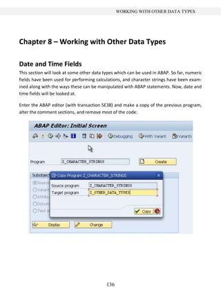
String Manipulation
Like many other programming languages, ABAP provides the functionality to interrogate
and manipulate the data held in character strings. This section will look at some of the
popular statements which ABAP provides for carrying out these functions:
Concatenating String Fields
Condensing Character Strings
Finding the Length of a String
Searching for Specific Characters
The SHIFT statement
Splitting Character Strings
SubFields
Concatenate
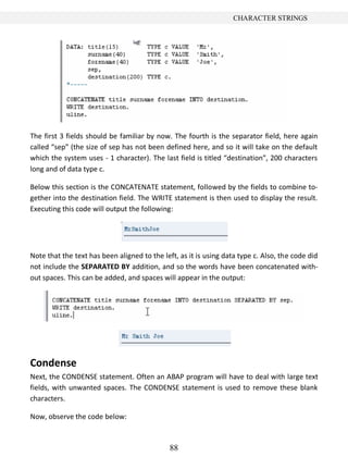
The concatenate statement allows two character strings to be joined so as to form a third
string. First, type the statement CONCATENATE into the program, and follow this by speci-
fying the fields, here “f1”, “f2” and so on. Then select the destination which the output
string should go to, here “d1”. If one adds a subsequent term, [separated by sep] (“sep”
here is an example name for the separator field), this will allow a specified value to be in-
serted between each field in the destination field:
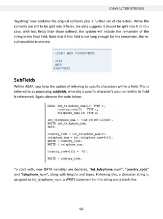
Note: If the destination field is shorter than the overall length of the input fields, the char-
acter string will be truncated to the length of the destination field, so ensure when using
the CONCATENATE statement, the string data type is being used, as these can hold over
65,000 characters.
As an example, observe the code in the image below.
87

88. CHARACTER STRINGS
The first 3 fields should be familiar by now. The fourth is the separator field, here again
called “sep” (the size of sep has not been defined here, and so it will take on the default
which the system uses - 1 character). The last field is titled “destination”, 200 characters
long and of data type c.
Below this section is the CONCATENATE statement, followed by the fields to combine to-
gether into the destination field. The WRITE statement is then used to display the result.
Executing this code will output the following:
Note that the text has been aligned to the left, as it is using data type c. Also, the code did
not include the SEPARATED BY addition, and so the words have been concatenated with-
out spaces. This can be added, and spaces will appear in the output:
Condense
Next, the CONDENSE statement. Often an ABAP program will have to deal with large text
fields, with unwanted spaces. The CONDENSE statement is used to remove these blank
characters.
Now, observe the code below:
88

89. CHARACTER STRINGS
This should, of course, be mostly familiar from the last section, with the addition of the
new, 20-character “spaced_name” field, with large spaces between the individual words.
Below we have an example of using the CONDENSE statement using our new variable:
The CONDENSE statement will remove the blank spaces between words in the variable,
leaving only 1 character’s space:
NO-GAPS
An optional addition to the CONDENSE statement is NO-GAPS, which as you may guess,
removes all spaces from our variable.
Find the Length of a String
To find the length of a string, a function rather than a statement is used. Added beneath
the previous data fields here, is a new one titled “len”, with a TYPE i, so as to just hold the
integer value of the string length.
89

90. CHARACTER STRINGS
The code to find the length of the ‘surname’ field and display it in the ‘len’ field appears
like this, with “strlen” defining the function:
The output, then, will appear like this:
Replace
Below I have created the “surname2” field and is 40 characters in length. Note that no
TYPE has been defined, so the system will use the default type, c:
Some text is then moved into the field after which the REPLACE statement is used to re-
place the comma with a period:
One thing to note here is that the REPLACE statement will only replace the first occurrence
in the string. So if, for example, the surname2 field read “Mr, Joe, Smith”, only the first
comma would be changed. All occurrences of comma’s could be replaced by making use
of a while loop, which will be discussed later on.
Search
Next, a look will be taken at searching for specific character strings within fields. Unsur-
prisingly, the statement SEARCH is used for this.
90

91. CHARACTER STRINGS
All that is needed is to enter SEARCH followed by the field which is to be searched, in this
instance the surname2 field. Then the string which is to be searched for, for example,
‘Joe’:
Note that here no variable has been declared to hold the result. In the case of the SEARCH
statement, two system variables are used. The first is “sy-subrc”, which identifies whether
the search was successful or not, and the second is “sy-fdpos”, which, if the search is suc-
cessful, is set to the position of the character string searched for in surname2. Below, a
small report is created to show the values of the system variables.
SEARCH Example 1
The first SEARCH statement, below, indicates that the surname2 field is being searched,
for the character string ‘Joe ‘. The Search statement will ignore the blank spaces. The
output will show the string being searched for, followed by the system variables and the
value results. In this case, the search should be successful.
SEARCH Example 2
The next example is very similar, but the full stops either side of ‘.Joe .’ mean that the
blank spaces this time will not be ignored and the system will search for the full string,
including the blanks. Here, the search will be unsuccessful, as the word ‘Joe’ in the
Surname2 field is not followed by four blank spaces.
91

92. CHARACTER STRINGS
SEARCH Example 3
This third search uses a wild card character ‘*’ and will search for any words ending in
‘ith’. This, again, should be successful.
SEARCH Example 4
The last example also uses the wild card facility, this time to search for words beginning
with ‘Smi’, which again should be successful. Compare the places in the code where the *
appears in this and the previous example.
Run a test on these searches, and output returns as follows:
When the sy-subrc = 0 this refers to a successful search. When sy-subrc = 4 in the second
example this indicates that the search was unsuccessful.
92

93. CHARACTER STRINGS
In the first search, the sy-fdpos value of 3 refers to the third character in the surname2
field, the offset, and the search term appears one character after this. The failure of the
second search means that a 0 is displayed in the sy-fdpos field. The value of 7 in the sy-
fdpos fields for the final two searches both mean that the word ‘Smith’ was found, corre-
sponding to the search terms, and that the searched word appears 1 character after the
offset value.
Shift
The SHIFT statement is a simple statement that allows one to move the contents of a
character string left or right, character by character. In this example, a field’s contents will
be moved to the left, deleting leading zeros. Declare a new DATA variable as follows:
“empl_num”, 10 characters long, and set the content of the field to ‘0000654321’, filling
all 10 characters of the field:
Using the SHIFT statement, then, the 4 zeros which begin this character string will be re-
moved, and the rest moved across to the left. Type the statement SHIFT, followed by the
field name. Define that it is to be shifted to the left, deleting leading zeros (don’t forget
the help screen can be used to view similar additions which can be added to this state-
ment). Then include a WRITE statement so that the result of the SHIFT statement can be
output. To the right of the number here, there will be four spaces, which have replaced
the leading zeros:
93

94. CHARACTER STRINGS
If no addition to the SHIFT statement is specified, the system will by default move every-
thing just one character to the left, leaving one space to the right:
The CIRCULAR addition to the SHIFT statement will cause, by default, everything to move
one space to the left again, but this time the character which is displaced at the beginning
of the statement will reappear at the end, rather than leaving a blank space:
Split
The SPLIT statement is used to separate the contents of a field into two or more fields.
Observe the code below:
94

95. CHARACTER STRINGS
The first section contains several DATA statements, “mystring”, “a1”, “a2”, “a3” and
“sep2”, along with their lengths and types. “Sep2” here is a separator field, with a value of
‘**’.
“mystring” is then given a value of ‘ 1234** ABCD **6789’, followed by a comment line
(which the program will ignore), then a WRITE statement, so that this initial value appears
in the output followed by a blank line, using the SKIP statement.
The SPLIT statement appears, followed by the name of the string which is to be split. The
AT addition appears next, telling the program that, where “sep2” appears (remember the
value of this is ‘**’), the field is to be split. Following this, the INTO then specifies the
fields which the split field is to be written to. The slightly odd positioning of the spaces in
the value of “mystring” will, when the statement is output, make clear the way that the
SPLIT statement populates the fields which the data is put into. Execute the code, and this
is the result:
You can see that the initial field has been split into a1, a2 and a3 exactly where the ** ap-
peared, leaving a leading space in the first two fields, but not in the third. Additionally, on
closer inspection there are blank spaces following the numbers in each field up to its de-
fined length, which is 10.
This next example shows the initial value of “mystring” now is made into a comment line,
and the comment line becomes part of the code:
95

96. CHARACTER STRINGS
‘mystring’ now contains the original contents plus a further set of characters. While the
contents are still to be split into 3 fields, the data suggests it should be split into 4. In this
case, with less fields than those defined, the system will include the remainder of the
string in the final field. Note that if this field is not long enough for the remainder, the re-
sult would be truncated.
SubFields
Within ABAP, you have the option of referring to specific characters within a field. This is
referred to as processing subfields, whereby a specific character’s position within its field
is referenced. Again, observe the code below:
To start with, new DATA variables are declared, “int_telephone_num”, “country_code”
and “telephone_num”, along with lengths and types. Following this, a character string is
assigned to int_telephone_num, a WRITE statement for this string and a blank line.
96

97. CHARACTER STRINGS
Next, the subfield processing appears. The first line states the country_code field is to be
filled with the first 3 characters of the int_telephone_num field, indicated by the number
in brackets.
Then, the field telephone_num is to be filled with 13 characters of the int_telephone_num
field, starting after the 4th character. The +4 part of the code here refers to where the field
is to begin. Then we have WRITE statements for both of the fields.
This last example indicates that the specific characters of int_telephone_num moved to
the country_code field will be replaced, after the first character, by the literal, 2-character
value ‘01’, showing that a subfield can itself be edited and updated without changing the
initial field. The results should look like this:
Subfields are regularly used in SAP to save time on creating unnecessary variables in
memory. It is just as easy to use the subfield syntax.
97

98. DEBUGGING PROGRAMS
Chapter 6 – Debugging Programs
This chapter will introduce the ABAP debugger, and will introduce some of the tools which
can be used to ensure that the programs you create function as intended. It will also show
ways to highlight logic bugs in programs that cannot be identified by the syntax checker.
The first step here is to load a program which has been used previously, and which ac-
cesses the database table which has been created regarding employee records. If you
have been following along with instructions, load program “Z_Employee_List_01” into the
ABAP Editor.
The program contains a number of SELECT loops, which in turn write the contents of the
table being read to the output screen in several ways, separated by ULINE statements:
Having examined the code, return to the front screen of the ABAP editor.
98

99. DEBUGGING PROGRAMS
Firstly, on this screen you will notice there is a ‘Debugging’ button in the toolbar (also ac-
cessible with SHIFT+F5):
Click this with the program name in the program input text box to start a new debugging
session. When this opens, a blue arrow should be visible, pointing at the first line of code
in the program:
An alternative way of starting a debugging session is to display the code itself from the
initial screen, select a line of code and set a breakpoint. This is done by, having selected a
line, clicking the Stop icon:
This sets a breakpoint for that line. When the program is then executed the execution will
pause highlighting the line that has the Breakpoint set entering the debugging session.
Usually, this is the easiest method to use, as one will often have a good idea of where the
99

100. DEBUGGING PROGRAMS
issues in a program are allowing you to focus on specific areas of code straight away,
rather than starting from the very beginning of a program as the previous method does:
There are two types of breakpoint which can be set in a program. Static (which will be ex-
amined later) and dynamic. A dynamic breakpoint is the kind which was used above, and
these are only valid for the current session. If one leaves the SAP GUI and returns later,
any dynamic breakpoints set will no longer exist. A breakpoint can also be set by double-
clicking any statement within the debugging session itself. To then remove these in the
session, simple double-click the stop icon appearing adjacent to them.
You will notice that a number of buttons appear at the top of the debugging screen:
These buttons allow for different modes of the ABAP debugger to be entered. The default
mode here is Fields.
The ‘Single step’ button, the first on the left in the row above the modes, also accessible
with F5, allows one to go through the code within the debugger line-by-line, or indeed as
its name would suggest, single steps. As one presses the button, the blue arrow on the left
of the code will move down one line at a time.
The next button along is the ‘Execute’ button, with a shortcut of F6. This allows for inde-
pendent sections of code to be executed, such as function modules or forms. This can be
very useful. If a program includes existing sections of code already created in an SAP sys-
100

101. DEBUGGING PROGRAMS
tem which are known to be correct, there is no need to debug them. These can then be
executed independently, while other parts are debugged to find specific problems.
The next button is the ‘Return’ function (F7). This can be very useful if one forgets to use
the ‘Execute’ function. If one goes through the lines of a program step-by-step, using the
F5 key to step into a working function module, which may contain many lines of code, it is
likely the case that it does not need to be debugged (because you know this function
module already exists). Pressing the F5 key endlessly to go through the lines of code here
is unnecessary when one wants to step out of this function module and access the parts
which require debugging. Using the ‘Return’ button, all of the code within a specific func-
tion can be executed, returning to the line of code which calls that function.
The fourth in the row is the ‘Continue’ option (F8). This allows one to continue the pro-
gram without going through step-by-step, line-by-line. When this button is pressed, the
program executes and the output screen is shown. This button can also be used to just
access a selected line of code, where the cursor is positioned. If one positions the cursor in
a line of code and presses continue, the blue arrow in the debugger will appear directly
next to that line. If you then press continue again, the program will be executed.
The next option in this row of the toolbar is ‘Display list’, accessible with CTRL+F12. This
takes you to the output screen as it currently stands within the debug session. Here, the
code has been executed to output the result of the first SELECT statement in the program:
This function allows you to see the results of the reports whilst the program is in mid-flow.
The last option here is ‘Create watchpoint’ (SHIFT + F8). Watchpoints will be returned to
soon.
101

102. DEBUGGING PROGRAMS
Fields mode
The ‘Fields’ mode of the ABAP debugger allows the contents of fields to be checked and
modified as the program is debugged. This can be accessed either by double-clicking the
field name within the code itself, or entering it into the ‘Field names’ section below the
code:
Note that, since here a table is involved, in the field name section the name of the table
must first be specified, followed by a -, then the name of the field. The field contents will
be filled in automatically. As you step through code line-by-line in the SELECT loop, the
text held in each field will change as each loop completes and moves onto the next record
in the table. This section allows for 8 fields to be monitored at any time. Fields 5 - 8 can be
made visible via the navigation buttons in the middle (to the right of the numbers 1 – 4).
Often when debugging a program, you may want to manually change the contents of
fields. This can be achieved by replacing the text in the field contents area, then clicking
the ‘Change field contents’ icon, marked with a pencil. Doing this can save a lot of time,
avoiding having to exit the debugging session multiple times to enter new values into
fields elsewhere:
102

103. DEBUGGING PROGRAMS
System Variables
At the bottom of the debugger screen, are 3 fields, named ‘SY-SUBRC’, ‘SY-TABIX’ and ‘SY-
DBCNT’:
Note that the value boxes here are greyed-out, meaning that they cannot be changed
manually. These are system fields, belonging to a table called SYST. This system table in-
cludes many system fields which are filled in at runtime. These system fields are filled in
automatically while the program is executed. Most statements within ABAP will cause
these system fields to be filled with 0 when executed successfully. It is important to re-
member that these fields are completely statement-dependent, meaning that they will
contain different values depending on which statement is executed. These system codes
and variables will be looked at in greater depth later.
Table Mode
The second mode along from the Fields button on the left of the screen is Table mode.
Click this button and the code remains, but the bottom section changes to include an ‘In-
ternal table’ entry, and a single row:
Internal tables have not yet been covered in depth, but, put simply; an internal table is a
table of records which is stored in memory while the program is running. Table mode al-
lows one to interrogate the records and fields of each record in an internal table. As with
103

104. DEBUGGING PROGRAMS
Fields mode, the internal table can either be double-clicked in the code, or manually en-
tered into the ‘Internal table’ box.
If one does this for “zemployees”, then, a new window appears, displaying the table
name, its individual fields and their contents:
Things do look slightly different to normal here, as a table structure is being shown, rather
than an actual internal table. This results in the debugger showing the table structure as
above, listing the individual fields numbered 1 – 6 and their contents. When viewing an
internal table in this mode, one will see a number of records for each internal table with
their contents. These records can then be double-clicked to move to the above layout,
showing the individual fields for each record. This will be returned to later.
In this screen, the code remains, but the area in which it is displayed is very small. One can
continue to interrogate the code line-by-line as before still, but this may prove difficult. It
is usually simpler to check Table mode for the information required, and then click back to
Fields mode to continue the debug session.
104

105. DEBUGGING PROGRAMS
Breakpoints
Click the Breakpoint mode button in the ABAP debugger screen. This allows you to see a
list of the individual breakpoints which have been set. Double-clicking any breakpoint in
the Breakpoints table will remove that breakpoint from the list:
This breakpoint table can be very useful, particularly when one is in a large program with
many breakpoints set. It allows one to review the breakpoint, and allows for the removal
of breakpoints which are no longer desired.
It is important to remember that breakpoints (and indeed Watchpoints) are only valid for
the length of the current debug session. When you exit your session, the breakpoints will
be deleted. However, an option does exist allowing you to save breakpoints (and, again,
Watchpoints) before closing a debug session, keeping them active for the next time the
program is to be debugged, saving the hassle of recreating them. This is done by entering
105

106. DEBUGGING PROGRAMS
the ‘Breakpoint’ menu in the top toolbar and choosing ‘Save’. All of the breakpoints saved
will then remain until they are manually removed, or until the end of your SAP session.
If one is in the ABAP editor, it is possible to see an overview of all the dynamic break-
points set in the program by accessing the following menu option: Utilities  Breakpoints
 Display:
106

107. DEBUGGING PROGRAMS
The options at the bottom of this breakpoint table allow one to delete selected break-
points without entering the debugger and breakpoints can be navigated to in the program
itself (within the ABAP editor) by double clicking them in this table.
Static Breakpoints
Static breakpoints were briefly alluded to earlier. These refer to a line of code written into
a program which forces the program to enter debug mode at the specific line chosen. To
do this, the statement BREAK-POINT is used. When the code is executed, the debug ses-
sion will start with the usual blue arrow cursor pointing at the location of the static break-
point.
107

108. DEBUGGING PROGRAMS
Once this statement is embedded in a program, it is active for all users. This is largely un-
desirable, as others running the program, who do not want to debug the code, would be
faced with the breakpoint set by an individual user. Be careful not to leave this statement
line in programs which will be transported to other systems.
Watchpoints
Click the Watchpoints button in the ABAP debugger. The program code will be visible
above the Watchpoints table in the lower half of the screen. Breakpoints have previously
been discussed, and can be very useful, but are not always the ideal tool to use to pause
code execution, interrogate the contents of individual fields and internal tables and ana-
lyse the program’s logic.
Imagine the program was processing a table containing 1000 records, and one wanted to
debug the logic only when a certain condition occurs. This condition is dependent upon
the data held in the records being processed. By using breakpoints, one would have to
debug each individual record, obviously taking a huge amount of time. Here, Watchpoints
become useful. Using these, one can tell the program to stop in the same manner that it
would for a breakpoint, but instead of stopping at a specific line of code, it would stop
based on the value in a field. In this example then, if this value occurred only in the 200 th
line of the table, a watchpoint would allow the first 199 records to be skipped over.
A watchpoint is created with the ‘Create watchpoint’ button, seen above the list of modes
in the Watchpoint mode screen, or with SHIFT + F8.
Once this is done, a dialogue box will appear, with the program name filled in automati-
cally. Here you need to enter the name of the field to be watched. In the
Z_EMPLOYEE_LIST_01 example here, we will enter the surname field. The format is TA-
BLE_NAME-FIELD_NAME. Next, the relational operator is to be set. In this example, a sur-
108

109. DEBUGGING PROGRAMS
name with the value “Mills” will be sought, so the operator here is an =. This can be se-
lected from a drop-down menu, where one can also view other potential relational opera-
tors. The bottom field, then, should be filled in with the value to be watched for.
Note that one does not have to use a specific value in the bottom field, but can get a
watchpoint to compare a field against another field within the program. To do this the
‘Comparison field’ box should be checked, and the field name typed into the box rather
than a specific value.
Click the green tick to continue and create the watchpoint, and the entry will have been
added to the list at the bottom of the screen:
109

110. DEBUGGING PROGRAMS
Observe the boxes below the Watchpoints list here. They are currently empty, but when
the program is executed, it will pause once a value of ‘Mills’ is reached in the ‘surname’
field and this will be included in the box.
The output before the program is executed looks like this:
Note that the surname Mills appears in the fifth row down. When the program is executed
with the ‘Mills’ watchpoint set, the first four records will be written to the screen before
pausing at the fifth, when Mills is displayed.
You will see that the blue arrow cursor has paused at the SELECT loop in the code.
110

111. DEBUGGING PROGRAMS
Enter zemployees-surname in the Fields mode of the debugger to view the contents of the
field. You will see the field contains “MILLS”. Also in the Watchpoints mode, the bottom
field will now be filled:
Ending a Debug Session
There are two ways to stop debugging a program. The first is to use the F8 key to run the
program all the way through to the end. Keep in mind though, that if any break or Watch-
points are set, the execution will likely pause and have to be started again, perhaps multi-
ple times. Also this method depends entirely upon the program executing successfully. If
any runtime errors are caused, the debug session will terminate and return you to the SAP
menu screen.
The alternative way of stopping the debugger is to enter the ‘Debugging’ menu and
choose ‘Restart’. This way, no more of the program will be executed, and you can return
to the ABAP Editor’s initial screen:
111

112. DEBUGGING PROGRAMS
112

113. ENHANCING DATABASE TABLES
Chapter 7: Working with Database Tables
Making a Copy of a Table
This chapter will look at ways in which one can change the transparent tables created ear-
lier. It is important to know how to do this, and the implications of adding and taking away
fields for the underlying data in a database table.
Let’s take a look at the ZEMPLOYEES table created in Chapter 2. In the SAP GUI, key in
transaction code SE11 to access the ABAP dictionary, then display the table:
It is important to realise that whenever one wants to change a database table, there is a
risk of losing data, especially where key fields in the table are being affected. The database
system itself will try to determine whether adjustments can be made by deleting and cre-
ating new items which change the underlying database catalogue, or whether what has
already defined has to be re-implemented.
Quite often, when working with large tables, one has to manage the manipulation of the
data oneself, so as to be sure that data is not lost. Deleting fields is quite a simple task, the
table structure and its contents can add certain complications. Before starting any data-
base change tasks, it is important to mitigate against as many risks as possible, and start
113

114. ENHANCING DATABASE TABLES
by using a copy of the database table, allowing one to test out any changes one may want
to make, without affecting the initial table and its underlying data.
When you copy a database table, it is only the structure itself which is copied, meaning
only its properties - fields and so on, not the actual data.
Step back to the initial SE11 screen. With ZEMPLOYEES in the Database table field, click
the Copy button, then give the new table of ZEMPLOYEES2. The ‘Create Object Directory
Entry’ box will appear and as before, select ‘Local Object’:
A copy of the table has now been created. Choose display at the SE11 screen and the copy
will appear. The table’s status will read as ‘New’. It must be activated, so click the ‘Change’
button (the Pencil icon in the toolbar), and then Activate:
Note that all of the fields in the table, since they have been copied, are already active. This
is why it is only the table itself which has to be activated here. If you try to look at the ta-
114

115. ENHANCING DATABASE TABLES
ble, you will find there are no contents, because only the structure was copied, not the
underlying data. To create records, from the ‘Utilities’ menu, select ‘Table Contents’ and
then ‘Create Entries’ to display the screen where the records for the table can be created
as before.
Insert some records, click the Contents button, and then view the new table:
115

116. ENHANCING DATABASE TABLES
Add New Fields
Next, a new field will be added. This will be a non-key field and will be called INITIALS.
Create a new Data element for this named ZINITIALS using forward navigation. For the
data element, set the short text to ‘Initials’ and set the domain to CHAR03 (a character
string of length 3). In the Field label boxes type ‘Initials’, then activate the Data element.
The table should now have a new field like this:
Create another 3 more new fields and configure them as follows:
Field Name ‘GENDER’
o Set the Data element to ‘ZGENDER’. Configure the data element as follows:
 Short text: ‘Gender’
 Domain: ‘CHAR01’
 Field labels set to ‘Gender’
SALARY
o Set the Data element to ZSALARY
 Short text: ‘Salary’
 Domain: ‘CURR9’ (This has a length of 9, with 2 decimal places)
 Field labels set to ‘Salary’.
One thing to note about the Salary field is that, because it is a currency, another field for
this currency must be created and attached to ZSALARY to indicate what currency the sal-
ary is in. If you try to activate the table without doing this, an error message will appear
asking for a reference field to specify the currency.
116

117. ENHANCING DATABASE TABLES
Create a new field called ECURRENCY. Currency fields should already exist in the system,
so the Data element here will be a pre-existing one named CURCY. Type this, press enter
and the remaining fields should fill in automatically, leaving the new section of the table
looking like this:
Next, the system must be told that the Salary field is referencing the Currency field. Above
the table will be able to see a tab labelled ‘Currency/Quantity Fields’. Click this and the
table will be shown with two boxes to be filled in for the Salary field, since it has already
been specified that the domain for this field is Currency. In the ‘Reference table’ column
enter the name of the table, ‘ZEMPLOYEES2’ and in the ‘Reference field’ column, the
name of the new Currency Key, ‘ECURRENCY’. Now the table can be activated error free.
Foreign Keys
As shown earlier enter a new record. You will see that the currency key does not offer any
kind of drop-down menu, here for this example, type GBP, indicating Great British Pounds:
117

118. ENHANCING DATABASE TABLES
Save the record, and then return to the design of the table, where we can now add some
error-checking to ensure that valid entries are made in the Currency key field.
To enable error-checking on the currency key field, we need to make use of a Foreign Key.
These are used to ensure that only valid values can be entered into a field. Use forward
navigation on the CURCY data element. Look at the Data type tab and you will see that the
data element refers to a standard SAP domain, WAERS:
Double-click the WAERS domain to use forward navigation again. Look at the ‘Value range’
tab in this window, a ‘Value table’ box is visible at the bottom, labelled TCURC:
118

119. ENHANCING DATABASE TABLES
A Value table can be used to determine the entries that can be made in the field based on
this domain. Double-click TCURC to again use forward navigation and this value table will
be displayed.
Use the data browser to look at the data in this table. If you scroll down, the GBP value
from before can be found, among a number of others. This table can be used to ensure
that, in future, only entries found in this table can be entered into our new table ZEM-
PLOYEES2
119

120. ENHANCING DATABASE TABLES
Return to the ‘Maintain table’ screen for ZEMPLOYEES2, highlight the ECURRENCY field,
and click the Foreign key button visible in the toolbar above:
Choose ‘Yes’ in the box which appears and a ‘Create Foreign Key’ window will emerge.
Type the short text ‘Check Currency Field’. A small table is visible, detailing the two key
fields from the TCURC table and the ZEMPLOYEES2 table. The option is available to ensure
that the foreign key matches both fields, so that when the user is allowed to select an en-
try, the records returned will only be valid for the Client which is being worked in.
Here though, the Client is not to be chosen as part of the key, so select the Check-box
‘Generic’ for the top row, which refers to the Client, and remove the text from the two
boxes on this row where this is possible. Then click the ‘Copy’ button. The foreign key will
be created:
120

121. ENHANCING DATABASE TABLES
Activate the table, and then browse the data. Now, select the currency key and either
press the F4 key or select the drop-down box that appears, displaying all valid entries for
this field. If you were in record change mode you will then be able to select a value from
the table and see it update your zemployees 2 record. Try it out and select USD (US Dol-
lar).
121

122. ENHANCING DATABASE TABLES
Append Structures
Having looked at foreign keys, the next thing to look at are Append structures. These can
be used to add additional fields. This is the preferred method for maintaining SAP deliv-
ered tables and quite often for customer-specific tables. If one does not use Append struc-
tures, problems can arise if, for example, a new version of SAP is used which does not cor-
respond with aspects of the tables already created, resulting in serious errors.
Append structures give a safe way to enhance tables. When these are used, the initial ta-
ble remains unchanged, removing any risk of changes being overwritten later if a different
version of SAP is used. Quite often, a table may have multiple Append structures applied
to it, because different development needs have arisen as time has gone by and people
have wanted to add further fields to the standard SAP tables.
In the SE11 Maintain Table screen, go to the ‘Append structure’ button on the right of the
top toolbar:
122

123. ENHANCING DATABASE TABLES
Click this, and the system will suggest a name, ZAZEMPLOYEES2 (note that this, again,
must begin with a Z). Accept this and you will be presented with what looks like an empty
table structure. Enter the Short text “Extra Fields For Employees”, and then move down to
the table.
Note that the first field now is called ‘Component’. This is where new fields are created.
However, it may be useful to differentiate between fields created in the main table, and
the new components created here in the Append structure. Since both must comply with
the customer name rules, where Z was used in the main table, here use ZZ.
For the first component, a ‘Department’ field will be created. Type in the ‘Component’ box
‘ZZDEPT’ and the same again in ‘Component type’. For this Component type, use forward
navigation in the same way that it was used for the Data element before, double-clicking
to create. Save the Append structure as a local object when prompted, and then select to
create a Data element when prompted subsequently.
The familiar data element screen will now appear. Type ‘Department’ for the short text,
use CHAR10 for the domain and ‘Department’ again for the Field labels, then activate the
data element. Step back to the Append structure screen, then Activate:
Return to the main table screen, where a new row displaying the Append structure will
have been created. To then access this structure, simply double-click the row. In Change
mode only the ‘.APPEND’ line will be visible by default, but in Display mode the fields cre-
ated within this will appear below:
123

124. ENHANCING DATABASE TABLES
This is a very useful way to add new fields to a table without affecting the structure of the
table itself. If one then browses the data as normal, a new column will have been called
‘Department’. Data can then be entered into this field just like it can for any other:
Include Structures
Include structures are similar to Append structures, with the main difference being that
they are re-usable objects and can be linked to many other tables, ABAP programs, dia-
logue programs and structures. It is important to keep in mind that Include structures
must be flat structures, meaning that they cannot hold any additional structure within
them, and that the maximum length of the fields within an include structure is 16 charac-
ters.
There is no Include structure button in the way that there is an Append structure button.
To create one, first ensure Change mode is selected. Where the cursor is placed is impor-
tant here, as wherever the cursor is when the Include structure is created, it will be cre-
ated one row above. If you want the Include structure to be part of the table key, it must
appear at the top, because all table fields used as a table key need to be grouped together
at the top. In this instance though, it will just be inserted above the Append structure.
Place the cursor on the ‘.APPEND’ row, select the ‘Edit’ menu, then ‘Include’ and ‘Insert’.
124

125. ENHANCING DATABASE TABLES
In the window that appears, enter ‘ZEMPL’ in the ‘Structure’ field and click the continue
button. A warning box will appear stating that this is not yet active, dismiss this, and the
Include structure should now appear in the table:
To add a field to this, use forward navigation as before, double-clicking where ‘.INCLUDE
ZEMPL’ appears, save and choose ‘Yes’ to create the structure. The screen which then ap-
pears is very similar to the Append structure screen.
Type the Short text “Employee Include” and begin to create a field (the boxes are, like in
the Append structure, labelled ‘Component’), this time for location, called ZZLOCAT, and
use ZLOCAT for the ‘Component type’. Use forward navigation again to create this Data
element with Short text ‘Location’, the domain CHAR10 and ‘Location’ again for the Field
labels, then Activate this as usual. Activate the Include structure once the field has been
created and return to the main table to see the Include structure located just where we
wanted it, above the Append structure:
Activate the table now, and view the contents. The Location column should now be visi-
ble, and these records can now be edited and created like any other:
125

126. ENHANCING DATABASE TABLES
If one switches to Display mode, the field created in the Include structure can be seen in
the context of the main table, albeit in a different colour:
126

127. ENHANCING DATABASE TABLES
In Change mode, these fields can be seen by selecting the ‘.INCLUDE’ row and clicking the
‘Expand include’ icon (the same works for the Append structure also):
Key Fields
If you want to add or remove fields which are designated key fields, then it is important to
take into consideration what will be going on in the database itself. All of the new ele-
ments which have been created for this table have their features applied by the system to
the ABAP dictionary, not the underlying database. When any key field is adjusted, the sys-
tem has to apply changes to the underlying database itself. If there is data in the table,
and key fields are changed, this can have unintended consequences.
127

128. ENHANCING DATABASE TABLES
If you introduce a new key field, this will probably not have a large effect. However, if one
makes a key field no longer a key field, this will require consideration, because if there is a
lot of data in the underlying database, by taking away a key field, duplicate records could
be introduced. Corrupt data or records being deleted from the table can also happen here.
Let’s see how we can add, remove and alter fields without these hazards.
Open the full ZEMPLOYEES2 table in the ABAP Dictionary ‘Maintain Table’ screen. Let’s
change the ‘Surname’ field by turning it into a key field.
Check the two boxes (key and Index) by ‘SURNAME’ and Activate the table. When you now
view the table contents, the surname column will be a darker colour, indicating that it is
now a key field. Beyond this though, it appears very little has changed:
Now, uncheck the boxes on the ‘Maintain Table’ screen, to make it no longer a key field.
When you try to activate the table an error message appears, refusing to activate the ta-
ble as data may be lost with the removal of a key field:
128

129. ENHANCING DATABASE TABLES
To activate the table against what seem to be the wishes of the system (after all, one
knows the data will be fine as the surname field has not been operating as a key field at
any point previously), a different transaction must be used.
From the ‘Utilities’ menu, select ‘Database utility’, or use transaction code SE14. A new
screen will appear:
This transaction lets us automatically adjust the data held in our table when making ad-
justments to the database table structure. Environments where tables are being worked
on may contain a huge number of records. With this in mind, this transaction can be exe-
cuted as a background process. However, for our example the ‘Direct’ option is the option
129

130. ENHANCING DATABASE TABLES
to choose because we know we have very few records in our database table. Select this,
and then click ‘Activate and adjust database’ with ‘Save data’ radio button selected. Say
‘Yes’ when the box asks “Request: ‘Adjust’” and notice the status bar should indicate the
success of this execution. Then, step back to the ‘Maintain Table’ screen and you will see
the table should be Active with the surname field no longer key.
To insert a new field as part of the table key, you must be able to adjust the location of
fields on the screen. For example, if you wanted to create a new field above the surname
field, you would highlight the row and then click the ‘Insert row’ icon in the toolbar. This
toolbar also includes ‘Cut’, ‘Copy’ and ‘Paste’ options, allowing for rows to be moved up
and down if there is a need to do this:
Deleting Fields
While infrequent, occasionally there may be a need to remove a field from a table. When
doing this, it is important to take special care, as data can be lost in the process. Certainly
in the case of key fields.
If, for example, the Currency key field was removed from our table, the foreign key rela-
tionship to the TCURC table would be removed. As the SALARY field has to have a related
Currency Key this would cause the table to no longer continue working, and likely make
the ZEMPLOYEES2 table become inactive.
When deleting fields it is important to ask oneself whether the data being held in the table
is being used elsewhere, and whether its deletion will have further consequences. If you
do try to delete fields which are being used elsewhere, the SAP system should try to pre-
vent this, or at least issue a stern warning. This is not necessarily to be relied upon though,
so always ensure to check manually what the effects of deletion are likely to be. Also, if
130

131. ENHANCING DATABASE TABLES
you do delete fields, the table will have to be adjusted via the SE14 transaction to be acti-
vated again.
Create a new field, above ‘.INCLUDE’, named ‘ZAWESOME’. Use a previously created Data
element, here ZTITLE just to save time, and activate the table:
Create a new record in the table. The data here is not important and will be deleted, so
the content can be anything:
131

132. ENHANCING DATABASE TABLES
Now, to delete the field, highlight it in the ‘Maintain Table’ screen, and click the ‘Remove
row’ icon, in the toolbar next to ‘Insert row’. The row will disappear, but when you try to
activate the table, an error message will appear:
Transaction SE14 must again be used to adjust the table so the change can be applied. Fol-
low the same steps as in the previous section to perform this task. Once this is complete,
view the table again. The column has disappeared, and the data which was contained
within it lost:
To see what happens when a key field is deleted, return to the ABAP Dictionary initial
screen and make a copy of ZEMPLOYEES2, called, unsurprisingly, ZEMPLOYEES3. Doing this
will allow the ZEMPLOYEES2 table to not be damaged in this risky procedure. Activate the
new table (which, don’t forget, will be empty of records). As before, again make the Sur-
name field a key field. Now create some records for this table:
132

133. ENHANCING DATABASE TABLES
To save time creating new records, the same data was replicated here, with only slight
changes to the key fields. Remember that it is only one key field per entry which must be
unique for that particularly record to be unique itself.
Now, the surname field will be deleted, and the effects of deleting this key field observed.
By removing this key field, the only unique data which will be held for each record will be
the Employee Number and Client. Since SMITH and SMITH2, and ANDREWS and AN-
DREWS-2 have the same Employee Number and Client, these will no longer hold unique
key field data, leaving duplicate records, which the system will not allow.
Remove the Surname field; try to activate the table, and error messages will appear. Go
through SE14 to adjust the table for activation. When you now view the table, the Sur-
name field is gone, and two records have been lost, leaving only one of the two records
for each of the two Employee Numbers used:
Deleting Tables
One will not often have to delete an entire database table, for largely the same reasons as
were outlined above for fields. If this does have to be done it is important to remember
that one’s own customer-specific tables are the only ones which can be deleted, SAP de-
livered tables cannot be deleted. Because ZEMPLOYEES3 has only just been created, and
nothing else depends on this table, it can be deleted without consequences.
To check whether a table can be deleted without causing unintended consequences else-
where in the system, return to the ABAP Dictionary’s initial screen. Because the original
ZEMPLOYEES table was used in the programs which have been created, use this as a test.
Insert this into the Database table field on the screen and then click the ‘Where-used list’
icon from the toolbar.
133

134. ENHANCING DATABASE TABLES
Once this is clicked, a dialogue box will appear offering a list of check-boxes. This will then
search all of the different areas of the SAP system selected for references to the table
ZEMPLOYEES. To execute this search click the Continue icon. Choose ‘Yes’ to the pop-up
box, and wait while the system compiles the search results, which here show that this ta-
ble is being used currently by 2 programs:
Having done this, one now knows that if the ZEMPLOYEES table were to be deleted, these
programs would become inactive. By double-clicking these entries, one can see the code
in the program where ZEMPLOYEES is referred to, and if you double-click on any line of
the program, it will open the program at that line of code in the ABAP Editor. The Where-
used button is a very useful tool, which can be invaluable not just when deleting pro-
grams, but in many other scenarios.
If you were to try to delete ZEMPLOYEES, the system would not allow this course of action
and would prevent it from happening until all the programs that are dependent upon it
were either edited to remove references or deleted altogether themselves.
Since nothing depends upon ZEMPLOYEES3, this can be deleted. With the correct name in
the ‘Database table’ field, click the ‘Delete’ button in the toolbar:
134

135. ENHANCING DATABASE TABLES
A box appears stating that the data contained in the table would also be deleted. If you
click the green tick icon this time, the system would return to the main screen with the
table still intact. If the middle button, illustrated with the trashcan icon is clicked, this will
proceed with the deletion. Once this is done, the status bar should confirm the action. If
you try to display the table now, it does not exist. Once the deletion is completed, it can-
not be undone:
135

136. WORKING WITH OTHER DATA TYPES
Chapter 8 – Working with Other Data Types
Date and Time Fields
This section will look at some other data types which can be used in ABAP. So far, numeric
fields have been used for performing calculations, and character strings have been exam-
ined along with the ways these can be manipulated with ABAP statements. Now, date and
time fields will be looked at.
Enter the ABAP editor (with transaction SE38) and make a copy of the previous program,
alter the comment sections, and remove most of the code:
136