This book provides an overview of Python libraries for data analysis and scientific computing. It covers core libraries like NumPy, pandas, matplotlib and IPython, which are essential for tasks like loading, cleaning, transforming and visualizing data. The book also teaches best practices for data analysis workflows in Python and key programming techniques.
![Python for Data Analysis
by Wes McKinney
Copyright © 2013 Wes McKinney. All rights reserved.
Printed in the United States of America.
Published by O’Reilly Media, Inc., 1005 Gravenstein Highway North, Sebastopol, CA 95472.
O’Reilly books may be purchased for educational, business, or sales promotional use. Online editions
are also available for most titles (http://my.safaribooksonline.com). For more information, contact our
corporate/institutional sales department: 800-998-9938 or corporate@oreilly.com.
Editors: Julie Steele and Meghan Blanchette
Production Editor: Melanie Yarbrough
Copyeditor: Teresa Exley
Proofreader: BIM Publishing Services
Indexer: BIM Publishing Services
Cover Designer: Karen Montgomery
Interior Designer: David Futato
Illustrator: Rebecca Demarest
October 2012: First Edition.
Revision History for the First Edition:
2012-10-05 First release
See http://oreilly.com/catalog/errata.csp?isbn=9781449319793 for release details.
Nutshell Handbook, the Nutshell Handbook logo, and the O’Reilly logo are registered trademarks of
O’Reilly Media, Inc. Python for Data Analysis, the cover image of a golden-tailed tree shrew, and related
trade dress are trademarks of O’Reilly Media, Inc.
Many of the designations used by manufacturers and sellers to distinguish their products are claimed as
trademarks. Where those designations appear in this book, and O’Reilly Media, Inc., was aware of a
trademark claim, the designations have been printed in caps or initial caps.
While every precaution has been taken in the preparation of this book, the publisher and author assume
no responsibility for errors or omissions, or for damages resulting from the use of the information con-
tained herein.
ISBN: 978-1-449-31979-3
[LSI]
1349356084](https://image.slidesharecdn.com/wesmckinney-pythonfordataanalysis-oreillymedia2012-221114102054-a802e8f3/85/Wes-McKinney-Python-for-Data-Analysis-O-Reilly-Media-2012-pdf-4-320.jpg)


![If you see a message for a different version of EPD or it doesn’t work at all, you will
need to clean up your Windows environment variables. On Windows 7 you can start
typing “environment variables” in the programs search field and select Edit environ
ment variables for your account. On Windows XP, you will have to go to Control
Panel > System > Advanced > Environment Variables. On the window that pops up,
you are looking for the Path variable. It needs to contain the following two directory
paths, separated by semicolons:
C:Python27;C:Python27Scripts
If you installed other versions of Python, be sure to delete any other Python-related
directories from both the system and user Path variables. After making a path alterna-
tion, you have to restart the command prompt for the changes to take effect.
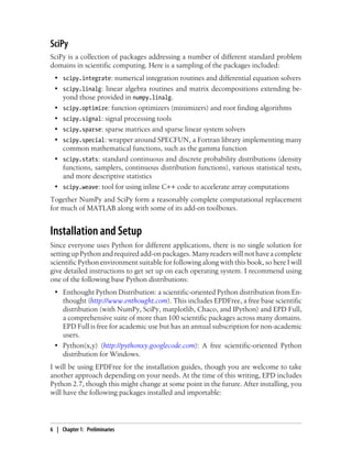
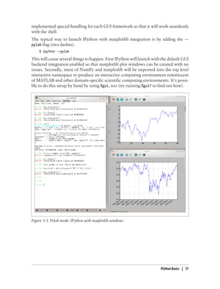
Once you can launch Python successfully from the command prompt, you need to
install pandas. The easiest way is to download the appropriate binary installer from
http://pypi.python.org/pypi/pandas. For EPDFree, this should be pandas-0.9.0.win32-
py2.7.exe. After you run this, let’s launch IPython and check that things are installed
correctly by importing pandas and making a simple matplotlib plot:
C:UsersWes>ipython --pylab
Python 2.7.3 |EPD_free 7.3-1 (32-bit)|
Type "copyright", "credits" or "license" for more information.
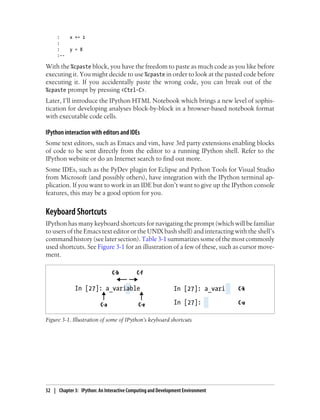
IPython 0.12.1 -- An enhanced Interactive Python.
? -> Introduction and overview of IPython's features.
%quickref -> Quick reference.
help -> Python's own help system.
object? -> Details about 'object', use 'object??' for extra details.
Welcome to pylab, a matplotlib-based Python environment [backend: WXAgg].
For more information, type 'help(pylab)'.
In [1]: import pandas
In [2]: plot(arange(10))
If successful, there should be no error messages and a plot window will appear. You
can also check that the IPython HTML notebook can be successfully run by typing:
$ ipython notebook --pylab=inline
If you use the IPython notebook application on Windows and normally
use Internet Explorer, you will likely need to install and run Mozilla
Firefox or Google Chrome instead.
EPDFree on Windows contains only 32-bit executables. If you want or need a 64-bit
setup on Windows, using EPD Full is the most painless way to accomplish that. If you
would rather install from scratch and not pay for an EPD subscription, Christoph
Gohlke at the University of California, Irvine, publishes unofficial binary installers for
8 | Chapter 1: Preliminaries](https://image.slidesharecdn.com/wesmckinney-pythonfordataanalysis-oreillymedia2012-221114102054-a802e8f3/85/Wes-McKinney-Python-for-Data-Analysis-O-Reilly-Media-2012-pdf-24-320.jpg)
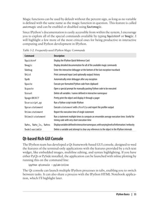
![$ ipython --pylab
22:29 ~/VirtualBox VMs/WindowsXP $ ipython
Python 2.7.3 |EPD_free 7.3-1 (32-bit)| (default, Apr 12 2012, 11:28:34)
Type "copyright", "credits" or "license" for more information.
IPython 0.12.1 -- An enhanced Interactive Python.
? -> Introduction and overview of IPython's features.
%quickref -> Quick reference.
help -> Python's own help system.
object? -> Details about 'object', use 'object??' for extra details.
Welcome to pylab, a matplotlib-based Python environment [backend: WXAgg].
For more information, type 'help(pylab)'.
In [1]: import pandas
In [2]: plot(arange(10))
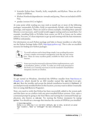
If this succeeds, a plot window with a straight line should pop up.
GNU/Linux
Some, but not all, Linux distributions include sufficiently up-to-date
versions of all the required Python packages and can be installed using
the built-in package management tool like apt. I detail setup using EPD-
Free as it's easily reproducible across distributions.
Linux details will vary a bit depending on your Linux flavor, but here I give details for
Debian-based GNU/Linux systems like Ubuntu and Mint. Setup is similar to OS X with
the exception of how EPDFree is installed. The installer is a shell script that must be
executed in the terminal. Depending on whether you have a 32-bit or 64-bit system,
you will either need to install the x86 (32-bit) or x86_64 (64-bit) installer. You will then
have a file named something similar to epd_free-7.3-1-rh5-x86_64.sh. To install it,
execute this script with bash:
$ bash epd_free-7.3-1-rh5-x86_64.sh
After accepting the license, you will be presented with a choice of where to put the
EPDFree files. I recommend installing the files in your home directory, say /home/wesm/
epd (substituting your own username for wesm).
Once the installer has finished, you need to add EPDFree’s bin directory to your
$PATH variable. If you are using the bash shell (the default in Ubuntu, for example), this
means adding the following path addition in your .bashrc:
export PATH=/home/wesm/epd/bin:$PATH
Obviously, substitute the installation directory you used for /home/wesm/epd/. After
doing this you can either start a new terminal process or execute your .bashrc again
with source ~/.bashrc.
10 | Chapter 1: Preliminaries](https://image.slidesharecdn.com/wesmckinney-pythonfordataanalysis-oreillymedia2012-221114102054-a802e8f3/85/Wes-McKinney-Python-for-Data-Analysis-O-Reilly-Media-2012-pdf-26-320.jpg)
![Code Examples
Most of the code examples in the book are shown with input and output as it would
appear executed in the IPython shell.
In [5]: code
Out[5]: output
At times, for clarity, multiple code examples will be shown side by side. These should
be read left to right and executed separately.
In [5]: code In [6]: code2
Out[5]: output Out[6]: output2
Data for Examples
Data sets for the examples in each chapter are hosted in a repository on GitHub: http:
//github.com/pydata/pydata-book. You can download this data either by using the git
revision control command-line program or by downloading a zip file of the repository
from the website.
I have made every effort to ensure that it contains everything necessary to reproduce
the examples, but I may have made some mistakes or omissions. If so, please send me
an e-mail: wesmckinn@gmail.com.
Import Conventions
The Python community has adopted a number of naming conventions for commonly-
used modules:
import numpy as np
import pandas as pd
import matplotlib.pyplot as plt
This means that when you see np.arange, this is a reference to the arange function in
NumPy. This is done as it’s considered bad practice in Python software development
to import everything (from numpy import *) from a large package like NumPy.
Jargon
I’ll use some terms common both to programming and data science that you may not
be familiar with. Thus, here are some brief definitions:
Munge/Munging/Wrangling
Describes the overall process of manipulating unstructured and/or messy data into
a structured or clean form. The word has snuck its way into the jargon of many
modern day data hackers. Munge rhymes with “lunge”.
Navigating This Book | 13](https://image.slidesharecdn.com/wesmckinney-pythonfordataanalysis-oreillymedia2012-221114102054-a802e8f3/85/Wes-McKinney-Python-for-Data-Analysis-O-Reilly-Media-2012-pdf-29-320.jpg)


![CHAPTER 2
Introductory Examples
This book teaches you the Python tools to work productively with data. While readers
may have many different end goals for their work, the tasks required generally fall into
a number of different broad groups:
Interacting with the outside world
Reading and writing with a variety of file formats and databases.
Preparation
Cleaning, munging, combining, normalizing, reshaping, slicing and dicing, and
transforming data for analysis.
Transformation
Applying mathematical and statistical operations to groups of data sets to derive
new data sets. For example, aggregating a large table by group variables.
Modeling and computation
Connecting your data to statistical models, machine learning algorithms, or other
computational tools
Presentation
Creating interactive or static graphical visualizations or textual summaries
In this chapter I will show you a few data sets and some things we can do with them.
These examples are just intended to pique your interest and thus will only be explained
at a high level. Don’t worry if you have no experience with any of these tools; they will
be discussed in great detail throughout the rest of the book. In the code examples you’ll
see input and output prompts like In [15]:; these are from the IPython shell.
1.usa.gov data from bit.ly
In 2011, URL shortening service bit.ly partnered with the United States government
website usa.gov to provide a feed of anonymous data gathered from users who shorten
links ending with .gov or .mil. As of this writing, in addition to providing a live feed,
hourly snapshots are available as downloadable text files.1
17](https://image.slidesharecdn.com/wesmckinney-pythonfordataanalysis-oreillymedia2012-221114102054-a802e8f3/85/Wes-McKinney-Python-for-Data-Analysis-O-Reilly-Media-2012-pdf-33-320.jpg)
![In the case of the hourly snapshots, each line in each file contains a common form of
web data known as JSON, which stands for JavaScript Object Notation. For example,
if we read just the first line of a file you may see something like
In [15]: path = 'ch02/usagov_bitly_data2012-03-16-1331923249.txt'
In [16]: open(path).readline()
Out[16]: '{ "a": "Mozilla/5.0 (Windows NT 6.1; WOW64) AppleWebKit/535.11
(KHTML, like Gecko) Chrome/17.0.963.78 Safari/535.11", "c": "US", "nk": 1,
"tz": "America/New_York", "gr": "MA", "g": "A6qOVH", "h": "wfLQtf", "l":
"orofrog", "al": "en-US,en;q=0.8", "hh": "1.usa.gov", "r":
"http://www.facebook.com/l/7AQEFzjSi/1.usa.gov/wfLQtf", "u":
"http://www.ncbi.nlm.nih.gov/pubmed/22415991", "t": 1331923247, "hc":
1331822918, "cy": "Danvers", "ll": [ 42.576698, -70.954903 ] }n'
Python has numerous built-in and 3rd party modules for converting a JSON string into
a Python dictionary object. Here I’ll use the json module and its loads function invoked
on each line in the sample file I downloaded:
import json
path = 'ch02/usagov_bitly_data2012-03-16-1331923249.txt'
records = [json.loads(line) for line in open(path)]
If you’ve never programmed in Python before, the last expression here is called a list
comprehension, which is a concise way of applying an operation (like json.loads) to a
collection of strings or other objects. Conveniently, iterating over an open file handle
gives you a sequence of its lines. The resulting object records is now a list of Python
dicts:
In [18]: records[0]
Out[18]:
{u'a': u'Mozilla/5.0 (Windows NT 6.1; WOW64) AppleWebKit/535.11 (KHTML, like
Gecko) Chrome/17.0.963.78 Safari/535.11',
u'al': u'en-US,en;q=0.8',
u'c': u'US',
u'cy': u'Danvers',
u'g': u'A6qOVH',
u'gr': u'MA',
u'h': u'wfLQtf',
u'hc': 1331822918,
u'hh': u'1.usa.gov',
u'l': u'orofrog',
u'll': [42.576698, -70.954903],
u'nk': 1,
u'r': u'http://www.facebook.com/l/7AQEFzjSi/1.usa.gov/wfLQtf',
u't': 1331923247,
u'tz': u'America/New_York',
u'u': u'http://www.ncbi.nlm.nih.gov/pubmed/22415991'}
1. http://www.usa.gov/About/developer-resources/1usagov.shtml
18 | Chapter 2: Introductory Examples](https://image.slidesharecdn.com/wesmckinney-pythonfordataanalysis-oreillymedia2012-221114102054-a802e8f3/85/Wes-McKinney-Python-for-Data-Analysis-O-Reilly-Media-2012-pdf-34-320.jpg)
![Note that Python indices start at 0 and not 1 like some other languages (like R). It’s
now easy to access individual values within records by passing a string for the key you
wish to access:
In [19]: records[0]['tz']
Out[19]: u'America/New_York'
The u here in front of the quotation stands for unicode, a standard form of string en-
coding. Note that IPython shows the time zone string object representation here rather
than its print equivalent:
In [20]: print records[0]['tz']
America/New_York
Counting Time Zones in Pure Python
Suppose we were interested in the most often-occurring time zones in the data set (the
tz field). There are many ways we could do this. First, let’s extract a list of time zones
again using a list comprehension:
In [25]: time_zones = [rec['tz'] for rec in records]
---------------------------------------------------------------------------
KeyError Traceback (most recent call last)
/home/wesm/book_scripts/whetting/<ipython> in <module>()
----> 1 time_zones = [rec['tz'] for rec in records]
KeyError: 'tz'
Oops! Turns out that not all of the records have a time zone field. This is easy to handle
as we can add the check if 'tz' in rec at the end of the list comprehension:
In [26]: time_zones = [rec['tz'] for rec in records if 'tz' in rec]
In [27]: time_zones[:10]
Out[27]:
[u'America/New_York',
u'America/Denver',
u'America/New_York',
u'America/Sao_Paulo',
u'America/New_York',
u'America/New_York',
u'Europe/Warsaw',
u'',
u'',
u'']
Just looking at the first 10 time zones we see that some of them are unknown (empty).
You can filter these out also but I’ll leave them in for now. Now, to produce counts by
time zone I’ll show two approaches: the harder way (using just the Python standard
library) and the easier way (using pandas). One way to do the counting is to use a dict
to store counts while we iterate through the time zones:
def get_counts(sequence):
counts = {}
1.usa.gov data from bit.ly | 19](https://image.slidesharecdn.com/wesmckinney-pythonfordataanalysis-oreillymedia2012-221114102054-a802e8f3/85/Wes-McKinney-Python-for-Data-Analysis-O-Reilly-Media-2012-pdf-35-320.jpg)
![for x in sequence:
if x in counts:
counts[x] += 1
else:
counts[x] = 1
return counts
If you know a bit more about the Python standard library, you might prefer to write
the same thing more briefly:
from collections import defaultdict
def get_counts2(sequence):
counts = defaultdict(int) # values will initialize to 0
for x in sequence:
counts[x] += 1
return counts
I put this logic in a function just to make it more reusable. To use it on the time zones,
just pass the time_zones list:
In [31]: counts = get_counts(time_zones)
In [32]: counts['America/New_York']
Out[32]: 1251
In [33]: len(time_zones)
Out[33]: 3440
If we wanted the top 10 time zones and their counts, we have to do a little bit of dic-
tionary acrobatics:
def top_counts(count_dict, n=10):
value_key_pairs = [(count, tz) for tz, count in count_dict.items()]
value_key_pairs.sort()
return value_key_pairs[-n:]
We have then:
In [35]: top_counts(counts)
Out[35]:
[(33, u'America/Sao_Paulo'),
(35, u'Europe/Madrid'),
(36, u'Pacific/Honolulu'),
(37, u'Asia/Tokyo'),
(74, u'Europe/London'),
(191, u'America/Denver'),
(382, u'America/Los_Angeles'),
(400, u'America/Chicago'),
(521, u''),
(1251, u'America/New_York')]
20 | Chapter 2: Introductory Examples](https://image.slidesharecdn.com/wesmckinney-pythonfordataanalysis-oreillymedia2012-221114102054-a802e8f3/85/Wes-McKinney-Python-for-Data-Analysis-O-Reilly-Media-2012-pdf-36-320.jpg)
![If you search the Python standard library, you may find the collections.Counter class,
which makes this task a lot easier:
In [49]: from collections import Counter
In [50]: counts = Counter(time_zones)
In [51]: counts.most_common(10)
Out[51]:
[(u'America/New_York', 1251),
(u'', 521),
(u'America/Chicago', 400),
(u'America/Los_Angeles', 382),
(u'America/Denver', 191),
(u'Europe/London', 74),
(u'Asia/Tokyo', 37),
(u'Pacific/Honolulu', 36),
(u'Europe/Madrid', 35),
(u'America/Sao_Paulo', 33)]
Counting Time Zones with pandas
The main pandas data structure is the DataFrame, which you can think of as repre-
senting a table or spreadsheet of data. Creating a DataFrame from the original set of
records is simple:
In [289]: from pandas import DataFrame, Series
In [290]: import pandas as pd
In [291]: frame = DataFrame(records)
In [292]: frame
Out[292]:
<class 'pandas.core.frame.DataFrame'>
Int64Index: 3560 entries, 0 to 3559
Data columns:
_heartbeat_ 120 non-null values
a 3440 non-null values
al 3094 non-null values
c 2919 non-null values
cy 2919 non-null values
g 3440 non-null values
gr 2919 non-null values
h 3440 non-null values
hc 3440 non-null values
hh 3440 non-null values
kw 93 non-null values
l 3440 non-null values
ll 2919 non-null values
nk 3440 non-null values
r 3440 non-null values
t 3440 non-null values
tz 3440 non-null values
1.usa.gov data from bit.ly | 21](https://image.slidesharecdn.com/wesmckinney-pythonfordataanalysis-oreillymedia2012-221114102054-a802e8f3/85/Wes-McKinney-Python-for-Data-Analysis-O-Reilly-Media-2012-pdf-37-320.jpg)
![u 3440 non-null values
dtypes: float64(4), object(14)
In [293]: frame['tz'][:10]
Out[293]:
0 America/New_York
1 America/Denver
2 America/New_York
3 America/Sao_Paulo
4 America/New_York
5 America/New_York
6 Europe/Warsaw
7
8
9
Name: tz
The output shown for the frame is the summary view, shown for large DataFrame ob-
jects. The Series object returned by frame['tz'] has a method value_counts that gives
us what we’re looking for:
In [294]: tz_counts = frame['tz'].value_counts()
In [295]: tz_counts[:10]
Out[295]:
America/New_York 1251
521
America/Chicago 400
America/Los_Angeles 382
America/Denver 191
Europe/London 74
Asia/Tokyo 37
Pacific/Honolulu 36
Europe/Madrid 35
America/Sao_Paulo 33
Then, we might want to make a plot of this data using plotting library, matplotlib. You
can do a bit of munging to fill in a substitute value for unknown and missing time zone
data in the records. The fillna function can replace missing (NA) values and unknown
(empty strings) values can be replaced by boolean array indexing:
In [296]: clean_tz = frame['tz'].fillna('Missing')
In [297]: clean_tz[clean_tz == ''] = 'Unknown'
In [298]: tz_counts = clean_tz.value_counts()
In [299]: tz_counts[:10]
Out[299]:
America/New_York 1251
Unknown 521
America/Chicago 400
America/Los_Angeles 382
America/Denver 191
Missing 120
22 | Chapter 2: Introductory Examples](https://image.slidesharecdn.com/wesmckinney-pythonfordataanalysis-oreillymedia2012-221114102054-a802e8f3/85/Wes-McKinney-Python-for-Data-Analysis-O-Reilly-Media-2012-pdf-38-320.jpg)
![Europe/London 74
Asia/Tokyo 37
Pacific/Honolulu 36
Europe/Madrid 35
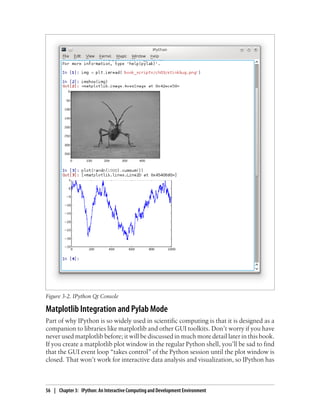
Making a horizontal bar plot can be accomplished using the plot method on the
counts objects:
In [301]: tz_counts[:10].plot(kind='barh', rot=0)
See Figure 2-1 for the resulting figure. We’ll explore more tools for working with this
kind of data. For example, the a field contains information about the browser, device,
or application used to perform the URL shortening:
In [302]: frame['a'][1]
Out[302]: u'GoogleMaps/RochesterNY'
In [303]: frame['a'][50]
Out[303]: u'Mozilla/5.0 (Windows NT 5.1; rv:10.0.2) Gecko/20100101 Firefox/10.0.2'
In [304]: frame['a'][51]
Out[304]: u'Mozilla/5.0 (Linux; U; Android 2.2.2; en-us; LG-P925/V10e Build/FRG83G) AppleWebKit/533.1 (K
Figure 2-1. Top time zones in the 1.usa.gov sample data
Parsing all of the interesting information in these “agent” strings may seem like a
daunting task. Luckily, once you have mastered Python’s built-in string functions and
regular expression capabilities, it is really not so bad. For example, we could split off
the first token in the string (corresponding roughly to the browser capability) and make
another summary of the user behavior:
In [305]: results = Series([x.split()[0] for x in frame.a.dropna()])
In [306]: results[:5]
Out[306]:
0 Mozilla/5.0
1 GoogleMaps/RochesterNY
2 Mozilla/4.0
3 Mozilla/5.0
4 Mozilla/5.0
1.usa.gov data from bit.ly | 23](https://image.slidesharecdn.com/wesmckinney-pythonfordataanalysis-oreillymedia2012-221114102054-a802e8f3/85/Wes-McKinney-Python-for-Data-Analysis-O-Reilly-Media-2012-pdf-39-320.jpg)
![In [307]: results.value_counts()[:8]
Out[307]:
Mozilla/5.0 2594
Mozilla/4.0 601
GoogleMaps/RochesterNY 121
Opera/9.80 34
TEST_INTERNET_AGENT 24
GoogleProducer 21
Mozilla/6.0 5
BlackBerry8520/5.0.0.681 4
Now, suppose you wanted to decompose the top time zones into Windows and non-
Windows users. As a simplification, let’s say that a user is on Windows if the string
'Windows' is in the agent string. Since some of the agents are missing, I’ll exclude these
from the data:
In [308]: cframe = frame[frame.a.notnull()]
We want to then compute a value whether each row is Windows or not:
In [309]: operating_system = np.where(cframe['a'].str.contains('Windows'),
.....: 'Windows', 'Not Windows')
In [310]: operating_system[:5]
Out[310]:
0 Windows
1 Not Windows
2 Windows
3 Not Windows
4 Windows
Name: a
Then, you can group the data by its time zone column and this new list of operating
systems:
In [311]: by_tz_os = cframe.groupby(['tz', operating_system])
The group counts, analogous to the value_counts function above, can be computed
using size. This result is then reshaped into a table with unstack:
In [312]: agg_counts = by_tz_os.size().unstack().fillna(0)
In [313]: agg_counts[:10]
Out[313]:
a Not Windows Windows
tz
245 276
Africa/Cairo 0 3
Africa/Casablanca 0 1
Africa/Ceuta 0 2
Africa/Johannesburg 0 1
Africa/Lusaka 0 1
America/Anchorage 4 1
America/Argentina/Buenos_Aires 1 0
24 | Chapter 2: Introductory Examples](https://image.slidesharecdn.com/wesmckinney-pythonfordataanalysis-oreillymedia2012-221114102054-a802e8f3/85/Wes-McKinney-Python-for-Data-Analysis-O-Reilly-Media-2012-pdf-40-320.jpg)
![America/Argentina/Cordoba 0 1
America/Argentina/Mendoza 0 1
Finally, let’s select the top overall time zones. To do so, I construct an indirect index
array from the row counts in agg_counts:
# Use to sort in ascending order
In [314]: indexer = agg_counts.sum(1).argsort()
In [315]: indexer[:10]
Out[315]:
tz
24
Africa/Cairo 20
Africa/Casablanca 21
Africa/Ceuta 92
Africa/Johannesburg 87
Africa/Lusaka 53
America/Anchorage 54
America/Argentina/Buenos_Aires 57
America/Argentina/Cordoba 26
America/Argentina/Mendoza 55
I then use take to select the rows in that order, then slice off the last 10 rows:
In [316]: count_subset = agg_counts.take(indexer)[-10:]
In [317]: count_subset
Out[317]:
a Not Windows Windows
tz
America/Sao_Paulo 13 20
Europe/Madrid 16 19
Pacific/Honolulu 0 36
Asia/Tokyo 2 35
Europe/London 43 31
America/Denver 132 59
America/Los_Angeles 130 252
America/Chicago 115 285
245 276
America/New_York 339 912
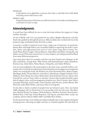
Then, as shown in the preceding code block, this can be plotted in a bar plot; I’ll make
it a stacked bar plot by passing stacked=True (see Figure 2-2) :
In [319]: count_subset.plot(kind='barh', stacked=True)
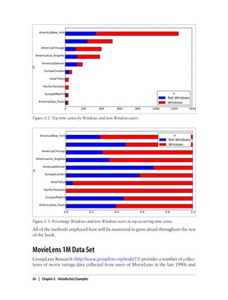
The plot doesn’t make it easy to see the relative percentage of Windows users in the
smaller groups, but the rows can easily be normalized to sum to 1 then plotted again
(see Figure 2-3):
In [321]: normed_subset = count_subset.div(count_subset.sum(1), axis=0)
In [322]: normed_subset.plot(kind='barh', stacked=True)
1.usa.gov data from bit.ly | 25](https://image.slidesharecdn.com/wesmckinney-pythonfordataanalysis-oreillymedia2012-221114102054-a802e8f3/85/Wes-McKinney-Python-for-Data-Analysis-O-Reilly-Media-2012-pdf-41-320.jpg)
![early 2000s. The data provide movie ratings, movie metadata (genres and year), and
demographic data about the users (age, zip code, gender, and occupation). Such data
is often of interest in the development of recommendation systems based on machine
learning algorithms. While I will not be exploring machine learning techniques in great
detail in this book, I will show you how to slice and dice data sets like these into the
exact form you need.
The MovieLens 1M data set contains 1 million ratings collected from 6000 users on
4000 movies. It’s spread across 3 tables: ratings, user information, and movie infor-
mation.Afterextractingthedatafromthezipfile,eachtablecanbeloadedintoapandas
DataFrame object using pandas.read_table:
import pandas as pd
unames = ['user_id', 'gender', 'age', 'occupation', 'zip']
users = pd.read_table('ml-1m/users.dat', sep='::', header=None,
names=unames)
rnames = ['user_id', 'movie_id', 'rating', 'timestamp']
ratings = pd.read_table('ml-1m/ratings.dat', sep='::', header=None,
names=rnames)
mnames = ['movie_id', 'title', 'genres']
movies = pd.read_table('ml-1m/movies.dat', sep='::', header=None,
names=mnames)
You can verify that everything succeeded by looking at the first few rows of each Da-
taFrame with Python's slice syntax:
In [334]: users[:5]
Out[334]:
user_id gender age occupation zip
0 1 F 1 10 48067
1 2 M 56 16 70072
2 3 M 25 15 55117
3 4 M 45 7 02460
4 5 M 25 20 55455
In [335]: ratings[:5]
Out[335]:
user_id movie_id rating timestamp
0 1 1193 5 978300760
1 1 661 3 978302109
2 1 914 3 978301968
3 1 3408 4 978300275
4 1 2355 5 978824291
In [336]: movies[:5]
Out[336]:
movie_id title genres
0 1 Toy Story (1995) Animation|Children's|Comedy
1 2 Jumanji (1995) Adventure|Children's|Fantasy
2 3 Grumpier Old Men (1995) Comedy|Romance
3 4 Waiting to Exhale (1995) Comedy|Drama
MovieLens 1M Data Set | 27](https://image.slidesharecdn.com/wesmckinney-pythonfordataanalysis-oreillymedia2012-221114102054-a802e8f3/85/Wes-McKinney-Python-for-Data-Analysis-O-Reilly-Media-2012-pdf-43-320.jpg)
![4 5 Father of the Bride Part II (1995) Comedy
In [337]: ratings
Out[337]:
<class 'pandas.core.frame.DataFrame'>
Int64Index: 1000209 entries, 0 to 1000208
Data columns:
user_id 1000209 non-null values
movie_id 1000209 non-null values
rating 1000209 non-null values
timestamp 1000209 non-null values
dtypes: int64(4)
Note that ages and occupations are coded as integers indicating groups described in
the data set’s README file. Analyzing the data spread across three tables is not a simple
task; for example, suppose you wanted to compute mean ratings for a particular movie
by sex and age. As you will see, this is much easier to do with all of the data merged
together into a single table. Using pandas’s merge function, we first merge ratings with
users then merging that result with the movies data. pandas infers which columns to
use as the merge (or join) keys based on overlapping names:
In [338]: data = pd.merge(pd.merge(ratings, users), movies)
In [339]: data
Out[339]:
<class 'pandas.core.frame.DataFrame'>
Int64Index: 1000209 entries, 0 to 1000208
Data columns:
user_id 1000209 non-null values
movie_id 1000209 non-null values
rating 1000209 non-null values
timestamp 1000209 non-null values
gender 1000209 non-null values
age 1000209 non-null values
occupation 1000209 non-null values
zip 1000209 non-null values
title 1000209 non-null values
genres 1000209 non-null values
dtypes: int64(6), object(4)
In [340]: data.ix[0]
Out[340]:
user_id 1
movie_id 1
rating 5
timestamp 978824268
gender F
age 1
occupation 10
zip 48067
title Toy Story (1995)
genres Animation|Children's|Comedy
Name: 0
28 | Chapter 2: Introductory Examples](https://image.slidesharecdn.com/wesmckinney-pythonfordataanalysis-oreillymedia2012-221114102054-a802e8f3/85/Wes-McKinney-Python-for-Data-Analysis-O-Reilly-Media-2012-pdf-44-320.jpg)
![In this form, aggregating the ratings grouped by one or more user or movie attributes
is straightforward once you build some familiarity with pandas. To get mean movie
ratings for each film grouped by gender, we can use the pivot_table method:
In [341]: mean_ratings = data.pivot_table('rating', rows='title',
.....: cols='gender', aggfunc='mean')
In [342]: mean_ratings[:5]
Out[342]:
gender F M
title
$1,000,000 Duck (1971) 3.375000 2.761905
'Night Mother (1986) 3.388889 3.352941
'Til There Was You (1997) 2.675676 2.733333
'burbs, The (1989) 2.793478 2.962085
...And Justice for All (1979) 3.828571 3.689024
This produced another DataFrame containing mean ratings with movie totals as row
labels and gender as column labels. First, I’m going to filter down to movies that re-
ceived at least 250 ratings (a completely arbitrary number); to do this, I group the data
by title and use size() to get a Series of group sizes for each title:
In [343]: ratings_by_title = data.groupby('title').size()
In [344]: ratings_by_title[:10]
Out[344]:
title
$1,000,000 Duck (1971) 37
'Night Mother (1986) 70
'Til There Was You (1997) 52
'burbs, The (1989) 303
...And Justice for All (1979) 199
1-900 (1994) 2
10 Things I Hate About You (1999) 700
101 Dalmatians (1961) 565
101 Dalmatians (1996) 364
12 Angry Men (1957) 616
In [345]: active_titles = ratings_by_title.index[ratings_by_title >= 250]
In [346]: active_titles
Out[346]:
Index(['burbs, The (1989), 10 Things I Hate About You (1999),
101 Dalmatians (1961), ..., Young Sherlock Holmes (1985),
Zero Effect (1998), eXistenZ (1999)], dtype=object)
The index of titles receiving at least 250 ratings can then be used to select rows from
mean_ratings above:
In [347]: mean_ratings = mean_ratings.ix[active_titles]
In [348]: mean_ratings
Out[348]:
<class 'pandas.core.frame.DataFrame'>
Index: 1216 entries, 'burbs, The (1989) to eXistenZ (1999)
MovieLens 1M Data Set | 29](https://image.slidesharecdn.com/wesmckinney-pythonfordataanalysis-oreillymedia2012-221114102054-a802e8f3/85/Wes-McKinney-Python-for-Data-Analysis-O-Reilly-Media-2012-pdf-45-320.jpg)
![Data columns:
F 1216 non-null values
M 1216 non-null values
dtypes: float64(2)
To see the top films among female viewers, we can sort by the F column in descending
order:
In [350]: top_female_ratings = mean_ratings.sort_index(by='F', ascending=False)
In [351]: top_female_ratings[:10]
Out[351]:
gender F M
Close Shave, A (1995) 4.644444 4.473795
Wrong Trousers, The (1993) 4.588235 4.478261
Sunset Blvd. (a.k.a. Sunset Boulevard) (1950) 4.572650 4.464589
Wallace & Gromit: The Best of Aardman Animation (1996) 4.563107 4.385075
Schindler's List (1993) 4.562602 4.491415
Shawshank Redemption, The (1994) 4.539075 4.560625
Grand Day Out, A (1992) 4.537879 4.293255
To Kill a Mockingbird (1962) 4.536667 4.372611
Creature Comforts (1990) 4.513889 4.272277
Usual Suspects, The (1995) 4.513317 4.518248
Measuring rating disagreement
Suppose you wanted to find the movies that are most divisive between male and female
viewers. One way is to add a column to mean_ratings containing the difference in
means, then sort by that:
In [352]: mean_ratings['diff'] = mean_ratings['M'] - mean_ratings['F']
Sorting by 'diff' gives us the movies with the greatest rating difference and which were
preferred by women:
In [353]: sorted_by_diff = mean_ratings.sort_index(by='diff')
In [354]: sorted_by_diff[:15]
Out[354]:
gender F M diff
Dirty Dancing (1987) 3.790378 2.959596 -0.830782
Jumpin' Jack Flash (1986) 3.254717 2.578358 -0.676359
Grease (1978) 3.975265 3.367041 -0.608224
Little Women (1994) 3.870588 3.321739 -0.548849
Steel Magnolias (1989) 3.901734 3.365957 -0.535777
Anastasia (1997) 3.800000 3.281609 -0.518391
Rocky Horror Picture Show, The (1975) 3.673016 3.160131 -0.512885
Color Purple, The (1985) 4.158192 3.659341 -0.498851
Age of Innocence, The (1993) 3.827068 3.339506 -0.487561
Free Willy (1993) 2.921348 2.438776 -0.482573
French Kiss (1995) 3.535714 3.056962 -0.478752
Little Shop of Horrors, The (1960) 3.650000 3.179688 -0.470312
Guys and Dolls (1955) 4.051724 3.583333 -0.468391
Mary Poppins (1964) 4.197740 3.730594 -0.467147
Patch Adams (1998) 3.473282 3.008746 -0.464536
30 | Chapter 2: Introductory Examples](https://image.slidesharecdn.com/wesmckinney-pythonfordataanalysis-oreillymedia2012-221114102054-a802e8f3/85/Wes-McKinney-Python-for-Data-Analysis-O-Reilly-Media-2012-pdf-46-320.jpg)
![Reversing the order of the rows and again slicing off the top 15 rows, we get the movies
preferred by men that women didn’t rate as highly:
# Reverse order of rows, take first 15 rows
In [355]: sorted_by_diff[::-1][:15]
Out[355]:
gender F M diff
Good, The Bad and The Ugly, The (1966) 3.494949 4.221300 0.726351
Kentucky Fried Movie, The (1977) 2.878788 3.555147 0.676359
Dumb & Dumber (1994) 2.697987 3.336595 0.638608
Longest Day, The (1962) 3.411765 4.031447 0.619682
Cable Guy, The (1996) 2.250000 2.863787 0.613787
Evil Dead II (Dead By Dawn) (1987) 3.297297 3.909283 0.611985
Hidden, The (1987) 3.137931 3.745098 0.607167
Rocky III (1982) 2.361702 2.943503 0.581801
Caddyshack (1980) 3.396135 3.969737 0.573602
For a Few Dollars More (1965) 3.409091 3.953795 0.544704
Porky's (1981) 2.296875 2.836364 0.539489
Animal House (1978) 3.628906 4.167192 0.538286
Exorcist, The (1973) 3.537634 4.067239 0.529605
Fright Night (1985) 2.973684 3.500000 0.526316
Barb Wire (1996) 1.585366 2.100386 0.515020
Suppose instead you wanted the movies that elicited the most disagreement among
viewers, independent of gender. Disagreement can be measured by the variance or
standard deviation of the ratings:
# Standard deviation of rating grouped by title
In [356]: rating_std_by_title = data.groupby('title')['rating'].std()
# Filter down to active_titles
In [357]: rating_std_by_title = rating_std_by_title.ix[active_titles]
# Order Series by value in descending order
In [358]: rating_std_by_title.order(ascending=False)[:10]
Out[358]:
title
Dumb & Dumber (1994) 1.321333
Blair Witch Project, The (1999) 1.316368
Natural Born Killers (1994) 1.307198
Tank Girl (1995) 1.277695
Rocky Horror Picture Show, The (1975) 1.260177
Eyes Wide Shut (1999) 1.259624
Evita (1996) 1.253631
Billy Madison (1995) 1.249970
Fear and Loathing in Las Vegas (1998) 1.246408
Bicentennial Man (1999) 1.245533
Name: rating
You may have noticed that movie genres are given as a pipe-separated (|) string. If you
wanted to do some analysis by genre, more work would be required to transform the
genre information into a more usable form. I will revisit this data later in the book to
illustrate such a transformation.
MovieLens 1M Data Set | 31](https://image.slidesharecdn.com/wesmckinney-pythonfordataanalysis-oreillymedia2012-221114102054-a802e8f3/85/Wes-McKinney-Python-for-Data-Analysis-O-Reilly-Media-2012-pdf-47-320.jpg)
![US Baby Names 1880-2010
The United States Social Security Administration (SSA) has made available data on the
frequency of baby names from 1880 through the present. Hadley Wickham, an author
of several popular R packages, has often made use of this data set in illustrating data
manipulation in R.
In [4]: names.head(10)
Out[4]:
name sex births year
0 Mary F 7065 1880
1 Anna F 2604 1880
2 Emma F 2003 1880
3 Elizabeth F 1939 1880
4 Minnie F 1746 1880
5 Margaret F 1578 1880
6 Ida F 1472 1880
7 Alice F 1414 1880
8 Bertha F 1320 1880
9 Sarah F 1288 1880
There are many things you might want to do with the data set:
• Visualize the proportion of babies given a particular name (your own, or another
name) over time.
• Determine the relative rank of a name.
• Determine the most popular names in each year or the names with largest increases
or decreases.
• Analyze trends in names: vowels, consonants, length, overall diversity, changes in
spelling, first and last letters
• Analyze external sources of trends: biblical names, celebrities, demographic
changes
Using the tools we’ve looked at so far, most of these kinds of analyses are very straight-
forward, so I will walk you through many of them. I encourage you to download and
explore the data yourself. If you find an interesting pattern in the data, I would love to
hear about it.
As of this writing, the US Social Security Administration makes available data files, one
per year, containing the total number of births for each sex/name combination. The
raw archive of these files can be obtained here:
http://www.ssa.gov/oact/babynames/limits.html
In the event that this page has been moved by the time you’re reading this, it can most
likely be located again by Internet search. After downloading the “National data” file
names.zip and unzipping it, you will have a directory containing a series of files like
yob1880.txt. I use the UNIX head command to look at the first 10 lines of one of the
files (on Windows, you can use the more command or open it in a text editor):
32 | Chapter 2: Introductory Examples](https://image.slidesharecdn.com/wesmckinney-pythonfordataanalysis-oreillymedia2012-221114102054-a802e8f3/85/Wes-McKinney-Python-for-Data-Analysis-O-Reilly-Media-2012-pdf-48-320.jpg)
![In [367]: !head -n 10 names/yob1880.txt
Mary,F,7065
Anna,F,2604
Emma,F,2003
Elizabeth,F,1939
Minnie,F,1746
Margaret,F,1578
Ida,F,1472
Alice,F,1414
Bertha,F,1320
Sarah,F,1288
As this is a nicely comma-separated form, it can be loaded into a DataFrame with
pandas.read_csv:
In [368]: import pandas as pd
In [369]: names1880 = pd.read_csv('names/yob1880.txt', names=['name', 'sex', 'births'])
In [370]: names1880
Out[370]:
<class 'pandas.core.frame.DataFrame'>
Int64Index: 2000 entries, 0 to 1999
Data columns:
name 2000 non-null values
sex 2000 non-null values
births 2000 non-null values
dtypes: int64(1), object(2)
These files only contain names with at least 5 occurrences in each year, so for simplic-
ity’s sake we can use the sum of the births column by sex as the total number of births
in that year:
In [371]: names1880.groupby('sex').births.sum()
Out[371]:
sex
F 90993
M 110493
Name: births
Since the data set is split into files by year, one of the first things to do is to assemble
all of the data into a single DataFrame and further to add a year field. This is easy to
do using pandas.concat:
# 2010 is the last available year right now
years = range(1880, 2011)
pieces = []
columns = ['name', 'sex', 'births']
for year in years:
path = 'names/yob%d.txt' % year
frame = pd.read_csv(path, names=columns)
frame['year'] = year
pieces.append(frame)
US Baby Names 1880-2010 | 33](https://image.slidesharecdn.com/wesmckinney-pythonfordataanalysis-oreillymedia2012-221114102054-a802e8f3/85/Wes-McKinney-Python-for-Data-Analysis-O-Reilly-Media-2012-pdf-49-320.jpg)
![# Concatenate everything into a single DataFrame
names = pd.concat(pieces, ignore_index=True)
There are a couple things to note here. First, remember that concat glues the DataFrame
objects together row-wise by default. Secondly, you have to pass ignore_index=True
because we’re not interested in preserving the original row numbers returned from
read_csv. So we now have a very large DataFrame containing all of the names data:
Now the names DataFrame looks like:
In [373]: names
Out[373]:
<class 'pandas.core.frame.DataFrame'>
Int64Index: 1690784 entries, 0 to 1690783
Data columns:
name 1690784 non-null values
sex 1690784 non-null values
births 1690784 non-null values
year 1690784 non-null values
dtypes: int64(2), object(2)
With this data in hand, we can already start aggregating the data at the year and sex
level using groupby or pivot_table, see Figure 2-4:
In [374]: total_births = names.pivot_table('births', rows='year',
.....: cols='sex', aggfunc=sum)
In [375]: total_births.tail()
Out[375]:
sex F M
year
2006 1896468 2050234
2007 1916888 2069242
2008 1883645 2032310
2009 1827643 1973359
2010 1759010 1898382
In [376]: total_births.plot(title='Total births by sex and year')
Next, let’s insert a column prop with the fraction of babies given each name relative to
the total number of births. A prop value of 0.02 would indicate that 2 out of every 100
babies was given a particular name. Thus, we group the data by year and sex, then add
the new column to each group:
def add_prop(group):
# Integer division floors
births = group.births.astype(float)
group['prop'] = births / births.sum()
return group
names = names.groupby(['year', 'sex']).apply(add_prop)
34 | Chapter 2: Introductory Examples](https://image.slidesharecdn.com/wesmckinney-pythonfordataanalysis-oreillymedia2012-221114102054-a802e8f3/85/Wes-McKinney-Python-for-Data-Analysis-O-Reilly-Media-2012-pdf-50-320.jpg)
![Remember that because births is of integer type, we have to cast either
the numerator or denominator to floating point to compute a fraction
(unless you are using Python 3!).
The resulting complete data set now has the following columns:
In [378]: names
Out[378]:
<class 'pandas.core.frame.DataFrame'>
Int64Index: 1690784 entries, 0 to 1690783
Data columns:
name 1690784 non-null values
sex 1690784 non-null values
births 1690784 non-null values
year 1690784 non-null values
prop 1690784 non-null values
dtypes: float64(1), int64(2), object(2)
When performing a group operation like this, it's often valuable to do a sanity check,
like verifying that the prop column sums to 1 within all the groups. Since this is floating
point data, use np.allclose to check that the group sums are sufficiently close to (but
perhaps not exactly equal to) 1:
In [379]: np.allclose(names.groupby(['year', 'sex']).prop.sum(), 1)
Out[379]: True
Now that this is done, I’m going to extract a subset of the data to facilitate further
analysis: the top 1000 names for each sex/year combination. This is yet another group
operation:
def get_top1000(group):
return group.sort_index(by='births', ascending=False)[:1000]
Figure 2-4. Total births by sex and year
US Baby Names 1880-2010 | 35](https://image.slidesharecdn.com/wesmckinney-pythonfordataanalysis-oreillymedia2012-221114102054-a802e8f3/85/Wes-McKinney-Python-for-Data-Analysis-O-Reilly-Media-2012-pdf-51-320.jpg)
![grouped = names.groupby(['year', 'sex'])
top1000 = grouped.apply(get_top1000)
If you prefer a do-it-yourself approach, you could also do:
pieces = []
for year, group in names.groupby(['year', 'sex']):
pieces.append(group.sort_index(by='births', ascending=False)[:1000])
top1000 = pd.concat(pieces, ignore_index=True)
The resulting data set is now quite a bit smaller:
In [382]: top1000
Out[382]:
<class 'pandas.core.frame.DataFrame'>
Int64Index: 261877 entries, 0 to 261876
Data columns:
name 261877 non-null values
sex 261877 non-null values
births 261877 non-null values
year 261877 non-null values
prop 261877 non-null values
dtypes: float64(1), int64(2), object(2)
We’ll use this Top 1,000 data set in the following investigations into the data.
Analyzing Naming Trends
With the full data set and Top 1,000 data set in hand, we can start analyzing various
naming trends of interest. Splitting the Top 1,000 names into the boy and girl portions
is easy to do first:
In [383]: boys = top1000[top1000.sex == 'M']
In [384]: girls = top1000[top1000.sex == 'F']
Simple time series, like the number of Johns or Marys for each year can be plotted but
require a bit of munging to be a bit more useful. Let’s form a pivot table of the total
number of births by year and name:
In [385]: total_births = top1000.pivot_table('births', rows='year', cols='name',
.....: aggfunc=sum)
Now, this can be plotted for a handful of names using DataFrame’s plot method:
In [386]: total_births
Out[386]:
<class 'pandas.core.frame.DataFrame'>
Int64Index: 131 entries, 1880 to 2010
Columns: 6865 entries, Aaden to Zuri
dtypes: float64(6865)
In [387]: subset = total_births[['John', 'Harry', 'Mary', 'Marilyn']]
In [388]: subset.plot(subplots=True, figsize=(12, 10), grid=False,
.....: title="Number of births per year")
36 | Chapter 2: Introductory Examples](https://image.slidesharecdn.com/wesmckinney-pythonfordataanalysis-oreillymedia2012-221114102054-a802e8f3/85/Wes-McKinney-Python-for-Data-Analysis-O-Reilly-Media-2012-pdf-52-320.jpg)
![See Figure 2-5 for the result. On looking at this, you might conclude that these names
have grown out of favor with the American population. But the story is actually more
complicated than that, as will be explored in the next section.
Figure 2-5. A few boy and girl names over time
Measuring the increase in naming diversity
One explanation for the decrease in plots above is that fewer parents are choosing
common names for their children. This hypothesis can be explored and confirmed in
the data. One measure is the proportion of births represented by the top 1000 most
popular names, which I aggregate and plot by year and sex:
In [390]: table = top1000.pivot_table('prop', rows='year',
.....: cols='sex', aggfunc=sum)
In [391]: table.plot(title='Sum of table1000.prop by year and sex',
.....: yticks=np.linspace(0, 1.2, 13), xticks=range(1880, 2020, 10))
See Figure 2-6 for this plot. So you can see that, indeed, there appears to be increasing
name diversity (decreasing total proportion in the top 1,000). Another interesting met-
ric is the number of distinct names, taken in order of popularity from highest to lowest,
in the top 50% of births. This number is a bit more tricky to compute. Let’s consider
just the boy names from 2010:
In [392]: df = boys[boys.year == 2010]
In [393]: df
Out[393]:
<class 'pandas.core.frame.DataFrame'>
Int64Index: 1000 entries, 260877 to 261876
Data columns:
US Baby Names 1880-2010 | 37](https://image.slidesharecdn.com/wesmckinney-pythonfordataanalysis-oreillymedia2012-221114102054-a802e8f3/85/Wes-McKinney-Python-for-Data-Analysis-O-Reilly-Media-2012-pdf-53-320.jpg)
![name 1000 non-null values
sex 1000 non-null values
births 1000 non-null values
year 1000 non-null values
prop 1000 non-null values
dtypes: float64(1), int64(2), object(2)
Figure 2-6. Proportion of births represented in top 1000 names by sex
After sorting prop in descending order, we want to know how many of the most popular
names it takes to reach 50%. You could write a for loop to do this, but a vectorized
NumPy way is a bit more clever. Taking the cumulative sum,cumsum, of prop then calling
themethodsearchsorted returnsthepositioninthecumulativesumatwhich0.5 would
need to be inserted to keep it in sorted order:
In [394]: prop_cumsum = df.sort_index(by='prop', ascending=False).prop.cumsum()
In [395]: prop_cumsum[:10]
Out[395]:
260877 0.011523
260878 0.020934
260879 0.029959
260880 0.038930
260881 0.047817
260882 0.056579
260883 0.065155
260884 0.073414
260885 0.081528
260886 0.089621
In [396]: prop_cumsum.searchsorted(0.5)
Out[396]: 116
38 | Chapter 2: Introductory Examples](https://image.slidesharecdn.com/wesmckinney-pythonfordataanalysis-oreillymedia2012-221114102054-a802e8f3/85/Wes-McKinney-Python-for-Data-Analysis-O-Reilly-Media-2012-pdf-54-320.jpg)
![Since arrays are zero-indexed, adding 1 to this result gives you a result of 117. By con-
trast, in 1900 this number was much smaller:
In [397]: df = boys[boys.year == 1900]
In [398]: in1900 = df.sort_index(by='prop', ascending=False).prop.cumsum()
In [399]: in1900.searchsorted(0.5) + 1
Out[399]: 25
It should now be fairly straightforward to apply this operation to each year/sex com-
bination; groupby those fields and apply a function returning the count for each group:
def get_quantile_count(group, q=0.5):
group = group.sort_index(by='prop', ascending=False)
return group.prop.cumsum().searchsorted(q) + 1
diversity = top1000.groupby(['year', 'sex']).apply(get_quantile_count)
diversity = diversity.unstack('sex')
This resulting DataFrame diversity now has two time series, one for each sex, indexed
by year. This can be inspected in IPython and plotted as before (see Figure 2-7):
In [401]: diversity.head()
Out[401]:
sex F M
year
1880 38 14
1881 38 14
1882 38 15
1883 39 15
1884 39 16
In [402]: diversity.plot(title="Number of popular names in top 50%")
Figure 2-7. Plot of diversity metric by year
US Baby Names 1880-2010 | 39](https://image.slidesharecdn.com/wesmckinney-pythonfordataanalysis-oreillymedia2012-221114102054-a802e8f3/85/Wes-McKinney-Python-for-Data-Analysis-O-Reilly-Media-2012-pdf-55-320.jpg)
![As you can see, girl names have always been more diverse than boy names, and they
have only become more so over time. Further analysis of what exactly is driving the
diversity, like the increase of alternate spellings, is left to the reader.
The “Last letter” Revolution
In 2007, a baby name researcher Laura Wattenberg pointed out on her website (http:
//www.babynamewizard.com) that the distribution of boy names by final letter has
changed significantly over the last 100 years. To see this, I first aggregate all of the births
in the full data set by year, sex, and final letter:
# extract last letter from name column
get_last_letter = lambda x: x[-1]
last_letters = names.name.map(get_last_letter)
last_letters.name = 'last_letter'
table = names.pivot_table('births', rows=last_letters,
cols=['sex', 'year'], aggfunc=sum)
Then, I select out three representative years spanning the history and print the first few
rows:
In [404]: subtable = table.reindex(columns=[1910, 1960, 2010], level='year')
In [405]: subtable.head()
Out[405]:
sex F M
year 1910 1960 2010 1910 1960 2010
last_letter
a 108376 691247 670605 977 5204 28438
b NaN 694 450 411 3912 38859
c 5 49 946 482 15476 23125
d 6750 3729 2607 22111 262112 44398
e 133569 435013 313833 28655 178823 129012
Next, normalize the table by total births to compute a new table containing proportion
of total births for each sex ending in each letter:
In [406]: subtable.sum()
Out[406]:
sex year
F 1910 396416
1960 2022062
2010 1759010
M 1910 194198
1960 2132588
2010 1898382
In [407]: letter_prop = subtable / subtable.sum().astype(float)
With the letter proportions now in hand, I can make bar plots for each sex broken
down by year. See Figure 2-8:
import matplotlib.pyplot as plt
40 | Chapter 2: Introductory Examples](https://image.slidesharecdn.com/wesmckinney-pythonfordataanalysis-oreillymedia2012-221114102054-a802e8f3/85/Wes-McKinney-Python-for-Data-Analysis-O-Reilly-Media-2012-pdf-56-320.jpg)
![fig, axes = plt.subplots(2, 1, figsize=(10, 8))
letter_prop['M'].plot(kind='bar', rot=0, ax=axes[0], title='Male')
letter_prop['F'].plot(kind='bar', rot=0, ax=axes[1], title='Female',
legend=False)
Figure 2-8. Proportion of boy and girl names ending in each letter
As you can see, boy names ending in “n” have experienced significant growth since the
1960s. Going back to the full table created above, I again normalize by year and sex
and select a subset of letters for the boy names, finally transposing to make each column
a time series:
In [410]: letter_prop = table / table.sum().astype(float)
In [411]: dny_ts = letter_prop.ix[['d', 'n', 'y'], 'M'].T
In [412]: dny_ts.head()
Out[412]:
d n y
year
1880 0.083055 0.153213 0.075760
1881 0.083247 0.153214 0.077451
1882 0.085340 0.149560 0.077537
1883 0.084066 0.151646 0.079144
1884 0.086120 0.149915 0.080405
With this DataFrame of time series in hand, I can make a plot of the trends over time
again with its plot method (see Figure 2-9):
In [414]: dny_ts.plot()
US Baby Names 1880-2010 | 41](https://image.slidesharecdn.com/wesmckinney-pythonfordataanalysis-oreillymedia2012-221114102054-a802e8f3/85/Wes-McKinney-Python-for-Data-Analysis-O-Reilly-Media-2012-pdf-57-320.jpg)
![Figure 2-9. Proportion of boys born with names ending in d/n/y over time
Boy names that became girl names (and vice versa)
Another fun trend is looking at boy names that were more popular with one sex earlier
in the sample but have “changed sexes” in the present. One example is the name Lesley
or Leslie. Going back to the top1000 dataset, I compute a list of names occurring in the
dataset starting with 'lesl':
In [415]: all_names = top1000.name.unique()
In [416]: mask = np.array(['lesl' in x.lower() for x in all_names])
In [417]: lesley_like = all_names[mask]
In [418]: lesley_like
Out[418]: array([Leslie, Lesley, Leslee, Lesli, Lesly], dtype=object)
From there, we can filter down to just those names and sum births grouped by name
to see the relative frequencies:
In [419]: filtered = top1000[top1000.name.isin(lesley_like)]
In [420]: filtered.groupby('name').births.sum()
Out[420]:
name
Leslee 1082
Lesley 35022
Lesli 929
Leslie 370429
Lesly 10067
Name: births
Next, let’s aggregate by sex and year and normalize within year:
42 | Chapter 2: Introductory Examples](https://image.slidesharecdn.com/wesmckinney-pythonfordataanalysis-oreillymedia2012-221114102054-a802e8f3/85/Wes-McKinney-Python-for-Data-Analysis-O-Reilly-Media-2012-pdf-58-320.jpg)
![In [421]: table = filtered.pivot_table('births', rows='year',
.....: cols='sex', aggfunc='sum')
In [422]: table = table.div(table.sum(1), axis=0)
In [423]: table.tail()
Out[423]:
sex F M
year
2006 1 NaN
2007 1 NaN
2008 1 NaN
2009 1 NaN
2010 1 NaN
Lastly, it’s now easy to make a plot of the breakdown by sex over time (Figure 2-10):
In [425]: table.plot(style={'M': 'k-', 'F': 'k--'})
Figure 2-10. Proportion of male/female Lesley-like names over time
Conclusions and The Path Ahead
The examples in this chapter are rather simple, but they’re here to give you a bit of a
flavor of what sorts of things you can expect in the upcoming chapters. The focus of
this book is on tools as opposed to presenting more sophisticated analytical methods.
Mastering the techniques in this book will enable you to implement your own analyses
(assuming you know what you want to do!) in short order.
Conclusions and The Path Ahead | 43](https://image.slidesharecdn.com/wesmckinney-pythonfordataanalysis-oreillymedia2012-221114102054-a802e8f3/85/Wes-McKinney-Python-for-Data-Analysis-O-Reilly-Media-2012-pdf-59-320.jpg)

![Since IPython has interactivity at its core, some of the features in this chapter are dif-
ficult to fully illustrate without a live console. If this is your first time learning about
IPython, I recommend that you follow along with the examples to get a feel for how
things work. As with any keyboard-driven console-like environment, developing mus-
cle-memory for the common commands is part of the learning curve.
Many parts of this chapter (for example: profiling and debugging) can
be safely omitted on a first reading as they are not necessary for under-
standing the rest of the book. This chapter is intended to provide a
standalone, rich overview of the functionality provided by IPython.
IPython Basics
You can launch IPython on the command line just like launching the regular Python
interpreter except with the ipython command:
$ ipython
Python 2.7.2 (default, May 27 2012, 21:26:12)
Type "copyright", "credits" or "license" for more information.
IPython 0.12 -- An enhanced Interactive Python.
? -> Introduction and overview of IPython's features.
%quickref -> Quick reference.
help -> Python's own help system.
object? -> Details about 'object', use 'object??' for extra details.
In [1]: a = 5
In [2]: a
Out[2]: 5
You can execute arbitrary Python statements by typing them in and pressing
<return>. When typing just a variable into IPython, it renders a string representation
of the object:
In [542]: data = {i : randn() for i in range(7)}
In [543]: data
Out[543]:
{0: 0.6900018528091594,
1: 1.0015434424937888,
2: -0.5030873913603446,
3: -0.6222742250596455,
4: -0.9211686080130108,
5: -0.726213492660829,
6: 0.2228955458351768}
46 | Chapter 3: IPython: An Interactive Computing and Development Environment](https://image.slidesharecdn.com/wesmckinney-pythonfordataanalysis-oreillymedia2012-221114102054-a802e8f3/85/Wes-McKinney-Python-for-Data-Analysis-O-Reilly-Media-2012-pdf-62-320.jpg)
![Many kinds of Python objects are formatted to be more readable, or pretty-printed,
which is distinct from normal printing with print. If you printed a dict like the above
in the standard Python interpreter, it would be much less readable:
>>> from numpy.random import randn
>>> data = {i : randn() for i in range(7)}
>>> print data
{0: -1.5948255432744511, 1: 0.10569006472787983, 2: 1.972367135977295,
3: 0.15455217573074576, 4: -0.24058577449429575, 5: -1.2904897053651216,
6: 0.3308507317325902}
IPython also provides facilities to make it easy to execute arbitrary blocks of code (via
somewhat glorified copy-and-pasting) and whole Python scripts. These will be dis-
cussed shortly.
Tab Completion
On the surface, the IPython shell looks like a cosmetically slightly-different interactive
Python interpreter. Users of Mathematica may find the enumerated input and output
prompts familiar. One of the major improvements over the standard Python shell is
tab completion, a feature common to most interactive data analysis environments.
While entering expressions in the shell, pressing <Tab> will search the namespace for
any variables (objects, functions, etc.) matching the characters you have typed so far:
In [1]: an_apple = 27
In [2]: an_example = 42
In [3]: an<Tab>
an_apple and an_example any
In this example, note that IPython displayed both the two variables I defined as well as
the Python keyword and and built-in function any. Naturally, you can also complete
methods and attributes on any object after typing a period:
In [3]: b = [1, 2, 3]
In [4]: b.<Tab>
b.append b.extend b.insert b.remove b.sort
b.count b.index b.pop b.reverse
The same goes for modules:
In [1]: import datetime
In [2]: datetime.<Tab>
datetime.date datetime.MAXYEAR datetime.timedelta
datetime.datetime datetime.MINYEAR datetime.tzinfo
datetime.datetime_CAPI datetime.time
IPython Basics | 47](https://image.slidesharecdn.com/wesmckinney-pythonfordataanalysis-oreillymedia2012-221114102054-a802e8f3/85/Wes-McKinney-Python-for-Data-Analysis-O-Reilly-Media-2012-pdf-63-320.jpg)
![Note that IPython by default hides methods and attributes starting with
underscores, such as magic methods and internal “private” methods
and attributes, in order to avoid cluttering the display (and confusing
new Python users!). These, too, can be tab-completed but you must first
type an underscore to see them. If you prefer to always see such methods
in tab completion, you can change this setting in the IPython configu-
ration.
Tab completion works in many contexts outside of searching the interactive namespace
and completing object or module attributes.When typing anything that looks like a file
path (even in a Python string), pressing <Tab> will complete anything on your com-
puter’s file system matching what you’ve typed:
In [3]: book_scripts/<Tab>
book_scripts/cprof_example.py book_scripts/ipython_script_test.py
book_scripts/ipython_bug.py book_scripts/prof_mod.py
In [3]: path = 'book_scripts/<Tab>
book_scripts/cprof_example.py book_scripts/ipython_script_test.py
book_scripts/ipython_bug.py book_scripts/prof_mod.py
Combined with the %run command (see later section), this functionality will undoubt-
edly save you many keystrokes.
Another area where tab completion saves time is in the completion of function keyword
arguments (including the = sign!).
Introspection
Using a question mark (?) before or after a variable will display some general informa-
tion about the object:
In [545]: b?
Type: list
String Form:[1, 2, 3]
Length: 3
Docstring:
list() -> new empty list
list(iterable) -> new list initialized from iterable's items
This is referred to as object introspection. If the object is a function or instance method,
the docstring, if defined, will also be shown. Suppose we’d written the following func-
tion:
def add_numbers(a, b):
"""
Add two numbers together
Returns
-------
the_sum : type of arguments
48 | Chapter 3: IPython: An Interactive Computing and Development Environment](https://image.slidesharecdn.com/wesmckinney-pythonfordataanalysis-oreillymedia2012-221114102054-a802e8f3/85/Wes-McKinney-Python-for-Data-Analysis-O-Reilly-Media-2012-pdf-64-320.jpg)
!["""
return a + b
Then using ? shows us the docstring:
In [547]: add_numbers?
Type: function
String Form:<function add_numbers at 0x5fad848>
File: book_scripts/<ipython-input-546-5473012eeb65>
Definition: add_numbers(a, b)
Docstring:
Add two numbers together
Returns
-------
the_sum : type of arguments
Using ?? will also show the function’s source code if possible:
In [548]: add_numbers??
Type: function
String Form:<function add_numbers at 0x5fad848>
File: book_scripts/<ipython-input-546-5473012eeb65>
Definition: add_numbers(a, b)
Source:
def add_numbers(a, b):
"""
Add two numbers together
Returns
-------
the_sum : type of arguments
"""
return a + b
? has a final usage, which is for searching the IPython namespace in a manner similar
to the standard UNIX or Windows command line. A number of characters combined
with the wildcard (*) will show all names matching the wildcard expression. For ex-
ample, we could get a list of all functions in the top level NumPy namespace containing
load:
In [549]: np.*load*?
np.load
np.loads
np.loadtxt
np.pkgload
The %run Command
Any file can be run as a Python program inside the environment of your IPython session
using the %run command. Suppose you had the following simple script stored in ipy
thon_script_test.py:
def f(x, y, z):
return (x + y) / z
a = 5
IPython Basics | 49](https://image.slidesharecdn.com/wesmckinney-pythonfordataanalysis-oreillymedia2012-221114102054-a802e8f3/85/Wes-McKinney-Python-for-Data-Analysis-O-Reilly-Media-2012-pdf-65-320.jpg)
![b = 6
c = 7.5
result = f(a, b, c)
This can be executed by passing the file name to %run:
In [550]: %run ipython_script_test.py
The script is run in an empty namespace (with no imports or other variables defined)
so that the behavior should be identical to running the program on the command line
using python script.py. All of the variables (imports, functions, and globals) defined
in the file (up until an exception, if any, is raised) will then be accessible in the IPython
shell:
In [551]: c
Out[551]: 7.5
In [552]: result
Out[552]: 1.4666666666666666
If a Python script expects command line arguments (to be found in sys.argv), these
can be passed after the file path as though run on the command line.
Should you wish to give a script access to variables already defined in
the interactive IPython namespace, use %run -i instead of plain %run.
Interrupting running code
Pressing <Ctrl-C> while any code is running, whether a script through %run or a long-
running command, will cause a KeyboardInterrupt to be raised. This will cause nearly
all Python programs to stop immediately except in very exceptional cases.
When a piece of Python code has called into some compiled extension
modules, pressing <Ctrl-C> will not cause the program execution to stop
immediately in all cases. In such cases, you will have to either wait until
control is returned to the Python interpreter, or, in more dire circum-
stances, forcibly terminate the Python process via the OS task manager.
Executing Code from the Clipboard
A quick-and-dirty way to execute code in IPython is via pasting from the clipboard.
This might seem fairly crude, but in practice it is very useful. For example, while de-
veloping a complex or time-consuming application, you may wish to execute a script
piece by piece, pausing at each stage to examine the currently loaded data and results.
Or, you might find a code snippet on the Internet that you want to run and play around
with, but you’d rather not create a new .py file for it.
50 | Chapter 3: IPython: An Interactive Computing and Development Environment](https://image.slidesharecdn.com/wesmckinney-pythonfordataanalysis-oreillymedia2012-221114102054-a802e8f3/85/Wes-McKinney-Python-for-Data-Analysis-O-Reilly-Media-2012-pdf-66-320.jpg)
![Code snippets can be pasted from the clipboard in many cases by pressing <Ctrl-Shift-
V>. Note that it is not completely robust as this mode of pasting mimics typing each
line into IPython, and line breaks are treated as <return>. This means that if you paste
code with an indented block and there is a blank line, IPython will think that the in-
dented block is over. Once the next line in the block is executed, an IndentationEr
ror will be raised. For example the following code:
x = 5
y = 7
if x > 5:
x += 1
y = 8
will not work if simply pasted:
In [1]: x = 5
In [2]: y = 7
In [3]: if x > 5:
...: x += 1
...:
In [4]: y = 8
IndentationError: unexpected indent
If you want to paste code into IPython, try the %paste and %cpaste
magic functions.
As the error message suggests, we should instead use the %paste and %cpaste magic
functions. %paste takes whatever text is in the clipboard and executes it as a single block
in the shell:
In [6]: %paste
x = 5
y = 7
if x > 5:
x += 1
y = 8
## -- End pasted text --
Depending on your platform and how you installed Python, there’s a
small chance that %paste will not work. Packaged distributions like
EPDFree (as described in in the intro) should not be a problem.
%cpaste is similar, except that it gives you a special prompt for pasting code into:
In [7]: %cpaste
Pasting code; enter '--' alone on the line to stop or use Ctrl-D.
:x = 5
:y = 7
:if x > 5:
IPython Basics | 51](https://image.slidesharecdn.com/wesmckinney-pythonfordataanalysis-oreillymedia2012-221114102054-a802e8f3/85/Wes-McKinney-Python-for-Data-Analysis-O-Reilly-Media-2012-pdf-67-320.jpg)
![Table 3-1. Standard IPython Keyboard Shortcuts
Command Description
Ctrl-P or up-arrow Search backward in command history for commands starting with currently-entered text
Ctrl-N or down-arrow Search forward in command history for commands starting with currently-entered text
Ctrl-R Readline-style reverse history search (partial matching)
Ctrl-Shift-V Paste text from clipboard
Ctrl-C Interrupt currently-executing code
Ctrl-A Move cursor to beginning of line
Ctrl-E Move cursor to end of line
Ctrl-K Delete text from cursor until end of line
Ctrl-U Discard all text on current line
Ctrl-F Move cursor forward one character
Ctrl-B Move cursor back one character
Ctrl-L Clear screen
Exceptions and Tracebacks
If an exception is raised while %run-ing a script or executing any statement, IPython will
by default print a full call stack trace (traceback) with a few lines of context around the
position at each point in the stack.
In [553]: %run ch03/ipython_bug.py
---------------------------------------------------------------------------
AssertionError Traceback (most recent call last)
/home/wesm/code/ipython/IPython/utils/py3compat.pyc in execfile(fname, *where)
176 else:
177 filename = fname
--> 178 __builtin__.execfile(filename, *where)
book_scripts/ch03/ipython_bug.py in <module>()
13 throws_an_exception()
14
---> 15 calling_things()
book_scripts/ch03/ipython_bug.py in calling_things()
11 def calling_things():
12 works_fine()
---> 13 throws_an_exception()
14
15 calling_things()
book_scripts/ch03/ipython_bug.py in throws_an_exception()
7 a = 5
8 b = 6
----> 9 assert(a + b == 10)
10
11 def calling_things():
AssertionError:
IPython Basics | 53](https://image.slidesharecdn.com/wesmckinney-pythonfordataanalysis-oreillymedia2012-221114102054-a802e8f3/85/Wes-McKinney-Python-for-Data-Analysis-O-Reilly-Media-2012-pdf-69-320.jpg)
![Having additional context by itself is a big advantage over the standard Python inter-
preter (which does not provide any additional context). The amount of context shown
can be controlled using the %xmode magic command, from minimal (same as the stan-
dard Python interpreter) to verbose (which inlines function argument values and more).
As you will see later in the chapter, you can step into the stack (using the %debug or
%pdb magics) after an error has occurred for interactive post-mortem debugging.
Magic Commands
IPython has many special commands, known as “magic” commands, which are de-
signed to faciliate common tasks and enable you to easily control the behavior of the
IPython system. A magic command is any command prefixed by the the percent symbol
%. For example, you can check the execution time of any Python statement, such as a
matrix multiplication, using the %timeit magic function (which will be discussed in
more detail later):
In [554]: a = np.random.randn(100, 100)
In [555]: %timeit np.dot(a, a)
10000 loops, best of 3: 69.1 us per loop
Magic commands can be viewed as command line programs to be run within the IPy-
thon system. Many of them have additional “command line” options, which can all be
viewed (as you might expect) using ?:
In [1]: %reset?
Resets the namespace by removing all names defined by the user.
Parameters
----------
-f : force reset without asking for confirmation.
-s : 'Soft' reset: Only clears your namespace, leaving history intact.
References to objects may be kept. By default (without this option),
we do a 'hard' reset, giving you a new session and removing all
references to objects from the current session.
Examples
--------
In [6]: a = 1
In [7]: a
Out[7]: 1
In [8]: 'a' in _ip.user_ns
Out[8]: True
In [9]: %reset -f
In [1]: 'a' in _ip.user_ns
Out[1]: False
54 | Chapter 3: IPython: An Interactive Computing and Development Environment](https://image.slidesharecdn.com/wesmckinney-pythonfordataanalysis-oreillymedia2012-221114102054-a802e8f3/85/Wes-McKinney-Python-for-Data-Analysis-O-Reilly-Media-2012-pdf-70-320.jpg)
![Using the Command History
IPython maintains a small on-disk database containing the text of each command that
you execute. This serves various purposes:
• Searching, completing, and executing previously-executed commands with mini-
mal typing
• Persisting the command history between sessions.
• Logging the input/output history to a file
Searching and Reusing the Command History
Being able to search and execute previous commands is, for many people, the most
useful feature. Since IPython encourages an iterative, interactive code development
workflow, you may often find yourself repeating the same commands, such as a %run
command or some other code snippet. Suppose you had run:
In[7]: %run first/second/third/data_script.py
and then explored the results of the script (assuming it ran successfully), only to find
that you made an incorrect calculation. After figuring out the problem and modifying
data_script.py, you can start typing a few letters of the %run command then press either
the <Ctrl-P> key combination or the <up arrow> key. This will search the command
history for the first prior command matching the letters you typed. Pressing either
<Ctrl-P> or <up arrow> multiple times will continue to search through the history. If
you pass over the command you wish to execute, fear not. You can move forward
through the command history by pressing either <Ctrl-N> or <down arrow>. After doing
this a few times you may start pressing these keys without thinking!
Using <Ctrl-R> gives you the same partial incremental searching capability provided
by the readline used in UNIX-style shells, such as the bash shell. On Windows, read
line functionality is emulated by IPython. To use this, press <Ctrl-R> then type a few
characters contained in the input line you want to search for:
In [1]: a_command = foo(x, y, z)
(reverse-i-search)`com': a_command = foo(x, y, z)
Pressing <Ctrl-R> will cycle through the history for each line matching the characters
you’ve typed.
Input and Output Variables
Forgetting to assign the result of a function call to a variable can be very annoying.
Fortunately, IPython stores references to both the input (the text that you type) and
output (the object that is returned) in special variables. The previous two outputs are
stored in the _ (one underscore) and __ (two underscores) variables, respectively:
58 | Chapter 3: IPython: An Interactive Computing and Development Environment](https://image.slidesharecdn.com/wesmckinney-pythonfordataanalysis-oreillymedia2012-221114102054-a802e8f3/85/Wes-McKinney-Python-for-Data-Analysis-O-Reilly-Media-2012-pdf-74-320.jpg)
![In [556]: 2 ** 27
Out[556]: 134217728
In [557]: _
Out[557]: 134217728
Input variables are stored in variables named like _iX, where X is the input line number.
For each such input variables there is a corresponding output variable _X. So after input
line 27, say, there will be two new variables _27 (for the output) and _i27 for the input.
In [26]: foo = 'bar'
In [27]: foo
Out[27]: 'bar'
In [28]: _i27
Out[28]: u'foo'
In [29]: _27
Out[29]: 'bar'
Since the input variables are strings, that can be executed again using the Python
exec keyword:
In [30]: exec _i27
Several magic functions allow you to work with the input and output history. %hist is
capable of printing all or part of the input history, with or without line numbers.
%reset is for clearing the interactive namespace and optionally the input and output
caches. The %xdel magic function is intended for removing all references to a particu-
lar object from the IPython machinery. See the documentation for both of these magics
for more details.
When working with very large data sets, keep in mind that IPython’s
input and output history causes any object referenced there to not be
garbage collected (freeing up the memory), even if you delete the vari-
ables from the interactive namespace using the del keyword. In such
cases, careful usage of %xdel and %reset can help you avoid running into
memory problems.
Logging the Input and Output
IPython is capable of logging the entire console session including input and output.
Logging is turned on by typing %logstart:
In [3]: %logstart
Activating auto-logging. Current session state plus future input saved.
Filename : ipython_log.py
Mode : rotate
Output logging : False
Raw input log : False
Using the Command History | 59](https://image.slidesharecdn.com/wesmckinney-pythonfordataanalysis-oreillymedia2012-221114102054-a802e8f3/85/Wes-McKinney-Python-for-Data-Analysis-O-Reilly-Media-2012-pdf-75-320.jpg)
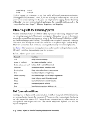
![In [2]: !python
Python 2.7.2 |EPD 7.1-2 (64-bit)| (default, Jul 3 2011, 15:17:51)
[GCC 4.1.2 20080704 (Red Hat 4.1.2-44)] on linux2
Type "packages", "demo" or "enthought" for more information.
>>>
The console output of a shell command can be stored in a variable by assigning the !-
escaped expression to a variable. For example, on my Linux-based machine connected
to the Internet via ethernet, I can get my IP address as a Python variable:
In [1]: ip_info = !ifconfig eth0 | grep "inet "
In [2]: ip_info[0].strip()
Out[2]: 'inet addr:192.168.1.137 Bcast:192.168.1.255 Mask:255.255.255.0'
The returned Python object ip_info is actually a custom list type containing various
versions of the console output.
IPython can also substitute in Python values defined in the current environment when
using !. To do this, preface the variable name by the dollar sign $:
In [3]: foo = 'test*'
In [4]: !ls $foo
test4.py test.py test.xml
The%alias magicfunctioncandefinecustomshortcutsforshellcommands.Asasimple
example:
In [1]: %alias ll ls -l
In [2]: ll /usr
total 332
drwxr-xr-x 2 root root 69632 2012-01-29 20:36 bin/
drwxr-xr-x 2 root root 4096 2010-08-23 12:05 games/
drwxr-xr-x 123 root root 20480 2011-12-26 18:08 include/
drwxr-xr-x 265 root root 126976 2012-01-29 20:36 lib/
drwxr-xr-x 44 root root 69632 2011-12-26 18:08 lib32/
lrwxrwxrwx 1 root root 3 2010-08-23 16:02 lib64 -> lib/
drwxr-xr-x 15 root root 4096 2011-10-13 19:03 local/
drwxr-xr-x 2 root root 12288 2012-01-12 09:32 sbin/
drwxr-xr-x 387 root root 12288 2011-11-04 22:53 share/
drwxrwsr-x 24 root src 4096 2011-07-17 18:38 src/
Multiple commands can be executed just as on the command line by separating them
with semicolons:
In [558]: %alias test_alias (cd ch08; ls; cd ..)
In [559]: test_alias
macrodata.csv spx.csv tips.csv
You’ll notice that IPython “forgets” any aliases you define interactively as soon as the
session is closed. To create permanent aliases, you will need to use the configuration
system. See later in the chapter.
Interacting with the Operating System | 61](https://image.slidesharecdn.com/wesmckinney-pythonfordataanalysis-oreillymedia2012-221114102054-a802e8f3/85/Wes-McKinney-Python-for-Data-Analysis-O-Reilly-Media-2012-pdf-77-320.jpg)
![Directory Bookmark System
IPython has a simple directory bookmarking system to enable you to save aliases for
common directories so that you can jump around very easily. For example, I’m an avid
user of Dropbox, so I can define a bookmark to make it easy to change directories to
my Dropbox:
In [6]: %bookmark db /home/wesm/Dropbox/
Once I’ve done this, when I use the %cd magic, I can use any bookmarks I’ve defined
In [7]: cd db
(bookmark:db) -> /home/wesm/Dropbox/
/home/wesm/Dropbox
If a bookmark name conflicts with a directory name in your current working directory,
you can use the -b flag to override and use the bookmark location. Using the -l option
with %bookmark lists all of your bookmarks:
In [8]: %bookmark -l
Current bookmarks:
db -> /home/wesm/Dropbox/
Bookmarks, unlike aliases, are automatically persisted between IPython sessions.
Software Development Tools
In addition to being a comfortable environment for interactive computing and data
exploration, IPython is well suited as a software development environment. In data
analysis applications, it’s important first to have correct code. Fortunately, IPython has
closely integrated and enhanced the built-in Python pdb debugger. Secondly you want
your code to be fast. For this IPython has easy-to-use code timing and profiling tools.
I will give an overview of these tools in detail here.
Interactive Debugger
IPython’s debugger enhancespdb with tab completion, syntax highlighting, and context
for each line in exception tracebacks. One of the best times to debug code is right after
an error has occurred. The %debug command, when entered immediately after an ex-
ception,invokesthe“post-mortem”debuggeranddropsyouintothestackframewhere
the exception was raised:
In [2]: run ch03/ipython_bug.py
---------------------------------------------------------------------------
AssertionError Traceback (most recent call last)
/home/wesm/book_scripts/ch03/ipython_bug.py in <module>()
13 throws_an_exception()
14
---> 15 calling_things()
/home/wesm/book_scripts/ch03/ipython_bug.py in calling_things()
62 | Chapter 3: IPython: An Interactive Computing and Development Environment](https://image.slidesharecdn.com/wesmckinney-pythonfordataanalysis-oreillymedia2012-221114102054-a802e8f3/85/Wes-McKinney-Python-for-Data-Analysis-O-Reilly-Media-2012-pdf-78-320.jpg)
![11 def calling_things():
12 works_fine()
---> 13 throws_an_exception()
14
15 calling_things()
/home/wesm/book_scripts/ch03/ipython_bug.py in throws_an_exception()
7 a = 5
8 b = 6
----> 9 assert(a + b == 10)
10
11 def calling_things():
AssertionError:
In [3]: %debug
> /home/wesm/book_scripts/ch03/ipython_bug.py(9)throws_an_exception()
8 b = 6
----> 9 assert(a + b == 10)
10
ipdb>
Once inside the debugger, you can execute arbitrary Python code and explore all of the
objects and data (which have been “kept alive” by the interpreter) inside each stack
frame. By default you start in the lowest level, where the error occurred. By pressing
u (up) and d (down), you can switch between the levels of the stack trace:
ipdb> u
> /home/wesm/book_scripts/ch03/ipython_bug.py(13)calling_things()
12 works_fine()
---> 13 throws_an_exception()
14
Executing the %pdb command makes it so that IPython automatically invokes the de-
bugger after any exception, a mode that many users will find especially useful.
It’s also easy to use the debugger to help develop code, especially when you wish to set
breakpoints or step through the execution of a function or script to examine the state
at each stage. There are several ways to accomplish this. The first is by using %run with
the -d flag, which invokes the debugger before executing any code in the passed script.
You must immediately press s (step) to enter the script:
In [5]: run -d ch03/ipython_bug.py
Breakpoint 1 at /home/wesm/book_scripts/ch03/ipython_bug.py:1
NOTE: Enter 'c' at the ipdb> prompt to start your script.
> <string>(1)<module>()
ipdb> s
--Call--
> /home/wesm/book_scripts/ch03/ipython_bug.py(1)<module>()
1---> 1 def works_fine():
2 a = 5
3 b = 6
Software Development Tools | 63](https://image.slidesharecdn.com/wesmckinney-pythonfordataanalysis-oreillymedia2012-221114102054-a802e8f3/85/Wes-McKinney-Python-for-Data-Analysis-O-Reilly-Media-2012-pdf-79-320.jpg)
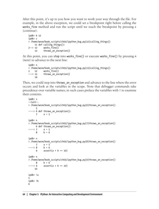
![Becoming proficient in the interactive debugger is largely a matter of practice and ex-
perience. See Table 3-3 for a full catalogue of the debugger commands. If you are used
to an IDE, you might find the terminal-driven debugger to be a bit bewildering at first,
but that will improve in time. Most of the Python IDEs have excellent GUI debuggers,
but it is usually a significant productivity gain to remain in IPython for your debugging.
Table 3-4. (I)Python debugger commands
Command Action
h(elp) Display command list
help command Show documentation for command
c(ontinue) Resume program execution
q(uit) Exit debugger without executing any more code
b(reak) number Set breakpoint at number in current file
b path/to/file.py:number Set breakpoint at line number in specified file
s(tep) Step into function call
n(ext) Execute current line and advance to next line at current level
u(p) / d(own) Move up/down in function call stack
a(rgs) Show arguments for current function
debug statement Invoke statement statement in new (recursive) debugger
l(ist) statement Show current position and context at current level of stack
w(here) Print full stack trace with context at current position
Other ways to make use of the debugger
There are a couple of other useful ways to invoke the debugger. The first is by using a
special set_trace function (named after pdb.set_trace), which is basically a “poor
man’s breakpoint”. Here are two small recipes you might want to put somewhere for
your general use (potentially adding them to your IPython profile as I do):
def set_trace():
from IPython.core.debugger import Pdb
Pdb(color_scheme='Linux').set_trace(sys._getframe().f_back)
def debug(f, *args, **kwargs):
from IPython.core.debugger import Pdb
pdb = Pdb(color_scheme='Linux')
return pdb.runcall(f, *args, **kwargs)
The first function, set_trace, is very simple. Put set_trace() anywhere in your code
that you want to stop and take a look around (for example, right before an exception
occurs):
In [7]: run ch03/ipython_bug.py
> /home/wesm/book_scripts/ch03/ipython_bug.py(16)calling_things()
15 set_trace()
Software Development Tools | 65](https://image.slidesharecdn.com/wesmckinney-pythonfordataanalysis-oreillymedia2012-221114102054-a802e8f3/85/Wes-McKinney-Python-for-Data-Analysis-O-Reilly-Media-2012-pdf-81-320.jpg)
![---> 16 throws_an_exception()
17
Pressing c (continue) will cause the code to resume normally with no harm done.
The debug function above enables you to invoke the interactive debugger easily on an
arbitrary function call. Suppose we had written a function like
def f(x, y, z=1):
tmp = x + y
return tmp / z
and we wished to step through its logic. Ordinarily using f would look like f(1, 2,
z=3). To instead step into f, pass f as the first argument to debug followed by the po-
sitional and keyword arguments to be passed to f:
In [6]: debug(f, 1, 2, z=3)
> <ipython-input>(2)f()
1 def f(x, y, z):
----> 2 tmp = x + y
3 return tmp / z
ipdb>
I find that these two simple recipes save me a lot of time on a day-to-day basis.
Lastly, the debugger can be used in conjunction with %run. By running a script with
%run -d, you will be dropped directly into the debugger, ready to set any breakpoints
and start the script:
In [1]: %run -d ch03/ipython_bug.py
Breakpoint 1 at /home/wesm/book_scripts/ch03/ipython_bug.py:1
NOTE: Enter 'c' at the ipdb> prompt to start your script.
> <string>(1)<module>()
ipdb>
Adding -b with a line number starts the debugger with a breakpoint set already:
In [2]: %run -d -b2 ch03/ipython_bug.py
Breakpoint 1 at /home/wesm/book_scripts/ch03/ipython_bug.py:2
NOTE: Enter 'c' at the ipdb> prompt to start your script.
> <string>(1)<module>()
ipdb> c
> /home/wesm/book_scripts/ch03/ipython_bug.py(2)works_fine()
1 def works_fine():
1---> 2 a = 5
3 b = 6
ipdb>
66 | Chapter 3: IPython: An Interactive Computing and Development Environment](https://image.slidesharecdn.com/wesmckinney-pythonfordataanalysis-oreillymedia2012-221114102054-a802e8f3/85/Wes-McKinney-Python-for-Data-Analysis-O-Reilly-Media-2012-pdf-82-320.jpg)
![Timing Code: %time and %timeit
For larger-scale or longer-running data analysis applications, you may wish to measure
the execution time of various components or of individual statements or function calls.
You may want a report of which functions are taking up the most time in a complex
process. Fortunately, IPython enables you to get this information very easily while you
are developing and testing your code.
Timing code by hand using the built-in time module and its functions time.clock and
time.time is often tedious and repetitive, as you must write the same uninteresting
boilerplate code:
import time
start = time.time()
for i in range(iterations):
# some code to run here
elapsed_per = (time.time() - start) / iterations
Since this is such a common operation, IPython has two magic functions %time and
%timeit to automate this process for you. %time runs a statement once, reporting the
total execution time. Suppose we had a large list of strings and we wanted to compare
different methods of selecting all strings starting with a particular prefix. Here is a
simple list of 700,000 strings and two identical methods of selecting only the ones that
start with 'foo':
# a very large list of strings
strings = ['foo', 'foobar', 'baz', 'qux',
'python', 'Guido Van Rossum'] * 100000
method1 = [x for x in strings if x.startswith('foo')]
method2 = [x for x in strings if x[:3] == 'foo']
It looks like they should be about the same performance-wise, right? We can check for
sure using %time:
In [561]: %time method1 = [x for x in strings if x.startswith('foo')]
CPU times: user 0.19 s, sys: 0.00 s, total: 0.19 s
Wall time: 0.19 s
In [562]: %time method2 = [x for x in strings if x[:3] == 'foo']
CPU times: user 0.09 s, sys: 0.00 s, total: 0.09 s
Wall time: 0.09 s
The Wall time is the main number of interest. So, it looks like the first method takes
more than twice as long, but it’s not a very precise measurement. If you try %time-ing
those statements multiple times yourself, you’ll find that the results are somewhat
variable. To get a more precise measurement, use the %timeit magic function. Given
an arbitrary statement, it has a heuristic to run a statement multiple times to produce
a fairly accurate average runtime.
In [563]: %timeit [x for x in strings if x.startswith('foo')]
10 loops, best of 3: 159 ms per loop
Software Development Tools | 67](https://image.slidesharecdn.com/wesmckinney-pythonfordataanalysis-oreillymedia2012-221114102054-a802e8f3/85/Wes-McKinney-Python-for-Data-Analysis-O-Reilly-Media-2012-pdf-83-320.jpg)
![In [564]: %timeit [x for x in strings if x[:3] == 'foo']
10 loops, best of 3: 59.3 ms per loop
This seemingly innocuous example illustrates that it is worth understanding the per-
formance characteristics of the Python standard library, NumPy, pandas, and other
libraries used in this book. In larger-scale data analysis applications, those milliseconds
will start to add up!
%timeit is especially useful for analyzing statements and functions with very short ex-
ecution times, even at the level of microseconds (1e-6 seconds) or nanoseconds (1e-9
seconds). These may seem like insignificant amounts of time, but of course a 20 mi-
crosecond function invoked 1 million times takes 15 seconds longer than a 5 micro-
second function. In the above example, we could very directly compare the two string
operations to understand their performance characteristics:
In [565]: x = 'foobar'
In [566]: y = 'foo'
In [567]: %timeit x.startswith(y)
1000000 loops, best of 3: 267 ns per loop
In [568]: %timeit x[:3] == y
10000000 loops, best of 3: 147 ns per loop
Basic Profiling: %prun and %run -p
Profiling code is closely related to timing code, except it is concerned with determining
where time is spent. The main Python profiling tool is the cProfile module, which is
not specific to IPython at all. cProfile executes a program or any arbitrary block of
code while keeping track of how much time is spent in each function.
A common way to use cProfile is on the command line, running an entire program
and outputting the aggregated time per function. Suppose we had a simple script which
does some linear algebra in a loop (computing the maximum absolute eigenvalues of
a series of 100 x 100 matrices):
import numpy as np
from numpy.linalg import eigvals
def run_experiment(niter=100):
K = 100
results = []
for _ in xrange(niter):
mat = np.random.randn(K, K)
max_eigenvalue = np.abs(eigvals(mat)).max()
results.append(max_eigenvalue)
return results
some_results = run_experiment()
print 'Largest one we saw: %s' % np.max(some_results)
68 | Chapter 3: IPython: An Interactive Computing and Development Environment](https://image.slidesharecdn.com/wesmckinney-pythonfordataanalysis-oreillymedia2012-221114102054-a802e8f3/85/Wes-McKinney-Python-for-Data-Analysis-O-Reilly-Media-2012-pdf-84-320.jpg)
![Don’t worry if you are not familiar with NumPy. You can run this script through
cProfile by running the following in the command line:
python -m cProfile cprof_example.py
If you try that, you’ll find that the results are outputted sorted by function name. This
makes it a bit hard to get an idea of where the most time is spent, so it’s very common
to specify a sort order using the -s flag:
$ python -m cProfile -s cumulative cprof_example.py
Largest one we saw: 11.923204422
15116 function calls (14927 primitive calls) in 0.720 seconds
Ordered by: cumulative time
ncalls tottime percall cumtime percall filename:lineno(function)
1 0.001 0.001 0.721 0.721 cprof_example.py:1(<module>)
100 0.003 0.000 0.586 0.006 linalg.py:702(eigvals)
200 0.572 0.003 0.572 0.003 {numpy.linalg.lapack_lite.dgeev}
1 0.002 0.002 0.075 0.075 __init__.py:106(<module>)
100 0.059 0.001 0.059 0.001 {method 'randn')
1 0.000 0.000 0.044 0.044 add_newdocs.py:9(<module>)
2 0.001 0.001 0.037 0.019 __init__.py:1(<module>)
2 0.003 0.002 0.030 0.015 __init__.py:2(<module>)
1 0.000 0.000 0.030 0.030 type_check.py:3(<module>)
1 0.001 0.001 0.021 0.021 __init__.py:15(<module>)
1 0.013 0.013 0.013 0.013 numeric.py:1(<module>)
1 0.000 0.000 0.009 0.009 __init__.py:6(<module>)
1 0.001 0.001 0.008 0.008 __init__.py:45(<module>)
262 0.005 0.000 0.007 0.000 function_base.py:3178(add_newdoc)
100 0.003 0.000 0.005 0.000 linalg.py:162(_assertFinite)
...
Only the first 15 rows of the output are shown. It’s easiest to read by scanning down
the cumtime column to see how much total time was spent inside each function. Note
that if a function calls some other function, the clock does not stop running. cProfile
records the start and end time of each function call and uses that to produce the timing.
In addition to the above command-line usage, cProfile can also be used programmat-
ically to profile arbitrary blocks of code without having to run a new process. IPython
has a convenient interface to this capability using the %prun command and the -p option
to %run. %prun takes the same “command line options” as cProfile but will profile an
arbitrary Python statement instead of a while .py file:
In [4]: %prun -l 7 -s cumulative run_experiment()
4203 function calls in 0.643 seconds
Ordered by: cumulative time
List reduced from 32 to 7 due to restriction <7>
ncalls tottime percall cumtime percall filename:lineno(function)
1 0.000 0.000 0.643 0.643 <string>:1(<module>)
1 0.001 0.001 0.643 0.643 cprof_example.py:4(run_experiment)
100 0.003 0.000 0.583 0.006 linalg.py:702(eigvals)
Software Development Tools | 69](https://image.slidesharecdn.com/wesmckinney-pythonfordataanalysis-oreillymedia2012-221114102054-a802e8f3/85/Wes-McKinney-Python-for-Data-Analysis-O-Reilly-Media-2012-pdf-85-320.jpg)
![200 0.569 0.003 0.569 0.003 {numpy.linalg.lapack_lite.dgeev}
100 0.058 0.001 0.058 0.001 {method 'randn'}
100 0.003 0.000 0.005 0.000 linalg.py:162(_assertFinite)
200 0.002 0.000 0.002 0.000 {method 'all' of 'numpy.ndarray' objects}
Similarly, calling %run -p -s cumulative cprof_example.py has the same effect as the
command-line approach above, except you never have to leave IPython.
Profiling a Function Line-by-Line
In some cases the information you obtain from %prun (or another cProfile-based profile
method) may not tell the whole story about a function’s execution time, or it may be
so complex that the results, aggregated by function name, are hard to interpret. For
this case, there is a small library called line_profiler (obtainable via PyPI or one of the
package management tools). It contains an IPython extension enabling a new magic
function %lprun that computes a line-by-line-profiling of one or more functions. You
can enable this extension by modifying your IPython configuration (see the IPython
documentation or the section on configuration later in this chapter) to include the
following line:
# A list of dotted module names of IPython extensions to load.
c.TerminalIPythonApp.extensions = ['line_profiler']
line_profiler can be used programmatically (see the full documentation), but it is
perhaps most powerful when used interactively in IPython. Suppose you had a module
prof_mod with the following code doing some NumPy array operations:
from numpy.random import randn
def add_and_sum(x, y):
added = x + y
summed = added.sum(axis=1)
return summed
def call_function():
x = randn(1000, 1000)
y = randn(1000, 1000)
return add_and_sum(x, y)
If we wanted to understand the performance of the add_and_sum function, %prun gives
us the following:
In [569]: %run prof_mod
In [570]: x = randn(3000, 3000)
In [571]: y = randn(3000, 3000)
In [572]: %prun add_and_sum(x, y)
4 function calls in 0.049 seconds
Ordered by: internal time
ncalls tottime percall cumtime percall filename:lineno(function)
1 0.036 0.036 0.046 0.046 prof_mod.py:3(add_and_sum)
70 | Chapter 3: IPython: An Interactive Computing and Development Environment](https://image.slidesharecdn.com/wesmckinney-pythonfordataanalysis-oreillymedia2012-221114102054-a802e8f3/85/Wes-McKinney-Python-for-Data-Analysis-O-Reilly-Media-2012-pdf-86-320.jpg)
![1 0.009 0.009 0.009 0.009 {method 'sum' of 'numpy.ndarray' objects}
1 0.003 0.003 0.049 0.049 <string>:1(<module>)
1 0.000 0.000 0.000 0.000 {method 'disable' of '_lsprof.Profiler' objects}
This is not especially enlightening. With the line_profiler IPython extension activa-
ted, a new command %lprun is available. The only difference in usage is that we must
instruct %lprun which function or functions we wish to profile. The general syntax is:
%lprun -f func1 -f func2 statement_to_profile
In this case, we want to profile add_and_sum, so we run:
In [573]: %lprun -f add_and_sum add_and_sum(x, y)
Timer unit: 1e-06 s
File: book_scripts/prof_mod.py
Function: add_and_sum at line 3
Total time: 0.045936 s
Line # Hits Time Per Hit % Time Line Contents
==============================================================
3 def add_and_sum(x, y):
4 1 36510 36510.0 79.5 added = x + y
5 1 9425 9425.0 20.5 summed = added.sum(axis=1)
6 1 1 1.0 0.0 return summed
You’ll probably agree this is much easier to interpret. In this case we profiled the same
function we used in the statement. Looking at the module code above, we could call
call_function and profile that as well as add_and_sum, thus getting a full picture of the
performance of the code:
In [574]: %lprun -f add_and_sum -f call_function call_function()
Timer unit: 1e-06 s
File: book_scripts/prof_mod.py
Function: add_and_sum at line 3
Total time: 0.005526 s
Line # Hits Time Per Hit % Time Line Contents
==============================================================
3 def add_and_sum(x, y):
4 1 4375 4375.0 79.2 added = x + y
5 1 1149 1149.0 20.8 summed = added.sum(axis=1)
6 1 2 2.0 0.0 return summed
File: book_scripts/prof_mod.py
Function: call_function at line 8
Total time: 0.121016 s
Line # Hits Time Per Hit % Time Line Contents
==============================================================
8 def call_function():
9 1 57169 57169.0 47.2 x = randn(1000, 1000)
10 1 58304 58304.0 48.2 y = randn(1000, 1000)
11 1 5543 5543.0 4.6 return add_and_sum(x, y)
As a general rule of thumb, I tend to prefer %prun (cProfile) for “macro” profiling and
%lprun (line_profiler) for “micro” profiling. It’s worthwhile to have a good under-
standing of both tools.
Software Development Tools | 71](https://image.slidesharecdn.com/wesmckinney-pythonfordataanalysis-oreillymedia2012-221114102054-a802e8f3/85/Wes-McKinney-Python-for-Data-Analysis-O-Reilly-Media-2012-pdf-87-320.jpg)
![The reason that you have to specify explicitly the names of the functions
you want to profile with %lprun is that the overhead of “tracing” the
execution time of each line is significant. Tracing functions that are not
of interest would potentially significantly alter the profile results.
IPython HTML Notebook
Starting in 2011, the IPython team, led by Brian Granger, built a web technology−based
interactive computational document format that is commonly known as the IPython
Notebook. It has grown into a wonderful tool for interactive computing and an ideal
medium for reproducible research and teaching. I’ve used it while writing most of the
examples in the book; I encourage you to make use of it, too.
It has a JSON-based .ipynb document format that enables easy sharing of code, output,
and figures. Recently in Python conferences, a popular approach for demonstrations
has been to use the notebook and post the .ipynb files online afterward for everyone
to play with.
The notebook application runs as a lightweight server process on the command line.
It can be started by running:
$ ipython notebook --pylab=inline
[NotebookApp] Using existing profile dir: u'/home/wesm/.config/ipython/profile_default'
[NotebookApp] Serving notebooks from /home/wesm/book_scripts
[NotebookApp] The IPython Notebook is running at: http://127.0.0.1:8888/
[NotebookApp] Use Control-C to stop this server and shut down all kernels.
On most platforms, your primary web browser will automatically open up to the note-
book dashboard. In some cases you may have to navigate to the listed URL. From there,
you can create a new notebook and start exploring.
Since you use the notebook inside a web browser, the server process can run anywhere.
You can even securely connect to notebooks running on cloud service providers like
Amazon EC2. As of this writing, a new project NotebookCloud (http://notebookcloud
.appspot.com) makes it easy to launch notebooks on EC2.
Tips for Productive Code Development Using IPython
Writing code in a way that makes it easy to develop, debug, and ultimately use inter-
actively may be a paradigm shift for many users. There are procedural details like code
reloading that may require some adjustment as well as coding style concerns.
As such, most of this section is more of an art than a science and will require some
experimentation on your part to determine a way to write your Python code that is
effective and productive for you. Ultimately you want to structure your code in a way
that makes it easy to use iteratively and to be able to explore the results of running a
program or function as effortlessly as possible. I have found software designed with
72 | Chapter 3: IPython: An Interactive Computing and Development Environment](https://image.slidesharecdn.com/wesmckinney-pythonfordataanalysis-oreillymedia2012-221114102054-a802e8f3/85/Wes-McKinney-Python-for-Data-Analysis-O-Reilly-Media-2012-pdf-88-320.jpg)
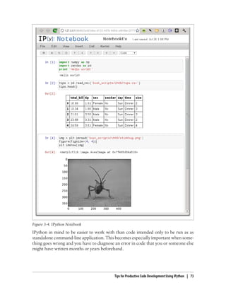
![Reloading Module Dependencies
In Python, when you type import some_lib, the code in some_lib is executed and all the
variables, functions, and imports defined within are stored in the newly created
some_lib module namespace. The next time you type import some_lib, you will get a
reference to the existing module namespace. The potential difficulty in interactive code
development in IPython comes when you, say, %run a script that depends on some other
module where you may have made changes. Suppose I had the following code in
test_script.py:
import some_lib
x = 5
y = [1, 2, 3, 4]
result = some_lib.get_answer(x, y)
If you were to execute %run test_script.py then modify some_lib.py, the next time you
execute %run test_script.py you will still get the old version of some_lib because of
Python’s “load-once” module system. This behavior differs from some other data anal-
ysis environments, like MATLAB, which automatically propagate code changes.1 To
cope with this, you have a couple of options. The first way is to use Python's built-in
reload function, altering test_script.py to look like the following:
import some_lib
reload(some_lib)
x = 5
y = [1, 2, 3, 4]
result = some_lib.get_answer(x, y)
This guarantees that you will get a fresh copy of some_lib every time you run
test_script.py. Obviously, if the dependencies go deeper, it might be a bit tricky to be
inserting usages of reload all over the place. For this problem, IPython has a special
dreload function (not a magic function) for “deep” (recursive) reloading of modules. If
I were to run import some_lib then type dreload(some_lib), it will attempt to reload
some_lib as well as all of its dependencies. This will not work in all cases, unfortunately,
but when it does it beats having to restart IPython.
Code Design Tips
There’s no simple recipe for this, but here are some high-level principles I have found
effective in my own work.
1. Since a module or package may be imported in many different places in a particular program, Python
caches a module’s code the first time it is imported rather than executing the code in the module every
time. Otherwise, modularity and good code organization could potentially cause inefficiency in an
application.
74 | Chapter 3: IPython: An Interactive Computing and Development Environment](https://image.slidesharecdn.com/wesmckinney-pythonfordataanalysis-oreillymedia2012-221114102054-a802e8f3/85/Wes-McKinney-Python-for-Data-Analysis-O-Reilly-Media-2012-pdf-90-320.jpg)
![Obviously, I don’t support taking this argument to the extreme, which would to be to
put all of your code in a single monstrous file. Finding a sensible and intuitive module
and package structure for a large codebase often takes a bit of work, but it is especially
important to get right in teams. Each module should be internally cohesive, and it
should be as obvious as possible where to find functions and classes responsible for
each area of functionality.
Advanced IPython Features
Making Your Own Classes IPython-friendly
IPython makes every effort to display a console-friendly string representation of any
object that you inspect. For many objects, like dicts, lists, and tuples, the built-in
pprint module is used to do the nice formatting. In user-defined classes, however, you
have to generate the desired string output yourself. Suppose we had the following sim-
ple class:
class Message:
def __init__(self, msg):
self.msg = msg
If you wrote this, you would be disappointed to discover that the default output for
your class isn’t very nice:
In [576]: x = Message('I have a secret')
In [577]: x
Out[577]: <__main__.Message instance at 0x60ebbd8>
IPython takes the string returned by the __repr__ magic method (by doing output =
repr(obj)) and prints that to the console. Thus, we can add a simple __repr__ method
to the above class to get a more helpful output:
class Message:
def __init__(self, msg):
self.msg = msg
def __repr__(self):
return 'Message: %s' % self.msg
In [579]: x = Message('I have a secret')
In [580]: x
Out[580]: Message: I have a secret
76 | Chapter 3: IPython: An Interactive Computing and Development Environment](https://image.slidesharecdn.com/wesmckinney-pythonfordataanalysis-oreillymedia2012-221114102054-a802e8f3/85/Wes-McKinney-Python-for-Data-Analysis-O-Reilly-Media-2012-pdf-92-320.jpg)
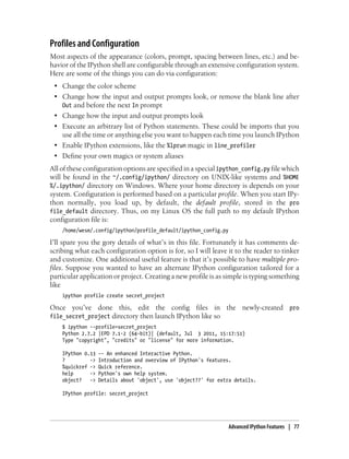
![In [1]:
As always, the online IPython documentation is an excellent resource for more on
profiles and configuration.
Credits
Parts of this chapter were derived from the wonderful documentation put together by
the IPython Development Team. I can’t thank them enough for all of their work build-
ing this amazing set of tools.
78 | Chapter 3: IPython: An Interactive Computing and Development Environment](https://image.slidesharecdn.com/wesmckinney-pythonfordataanalysis-oreillymedia2012-221114102054-a802e8f3/85/Wes-McKinney-Python-for-Data-Analysis-O-Reilly-Media-2012-pdf-94-320.jpg)
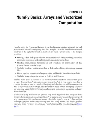
![For most data analysis applications, the main areas of functionality I’ll focus on are:
• Fast vectorized array operations for data munging and cleaning, subsetting and
filtering, transformation, and any other kinds of computations
• Common array algorithms like sorting, unique, and set operations
• Efficient descriptive statistics and aggregating/summarizing data
• Data alignment and relational data manipulations for merging and joining together
heterogeneous data sets
• Expressing conditional logic as array expressions instead of loops with if-elif-
else branches
• Group-wise data manipulations (aggregation, transformation, function applica-
tion). Much more on this in Chapter 5
While NumPy provides the computational foundation for these operations, you will
likely want to use pandas as your basis for most kinds of data analysis (especially for
structured or tabular data) as it provides a rich, high-level interface making most com-
mon data tasks very concise and simple. pandas also provides some more domain-
specific functionality like time series manipulation, which is not present in NumPy.
In this chapter and throughout the book, I use the standard NumPy
convention of always using import numpy as np. You are, of course,
welcome to put from numpy import * in your code to avoid having to
write np., but I would caution you against making a habit of this.
The NumPy ndarray: A Multidimensional Array Object
One of the key features of NumPy is its N-dimensional array object, or ndarray, which
is a fast, flexible container for large data sets in Python. Arrays enable you to perform
mathematical operations on whole blocks of data using similar syntax to the equivalent
operations between scalar elements:
In [8]: data
Out[8]:
array([[ 0.9526, -0.246 , -0.8856],
[ 0.5639, 0.2379, 0.9104]])
In [9]: data * 10 In [10]: data + data
Out[9]: Out[10]:
array([[ 9.5256, -2.4601, -8.8565], array([[ 1.9051, -0.492 , -1.7713],
[ 5.6385, 2.3794, 9.104 ]]) [ 1.1277, 0.4759, 1.8208]])
An ndarray is a generic multidimensional container for homogeneous data; that is, all
of the elements must be the same type. Every array has a shape, a tuple indicating the
size of each dimension, and a dtype, an object describing the data type of the array:
In [11]: data.shape
Out[11]: (2, 3)
80 | Chapter 4: NumPy Basics: Arrays and Vectorized Computation](https://image.slidesharecdn.com/wesmckinney-pythonfordataanalysis-oreillymedia2012-221114102054-a802e8f3/85/Wes-McKinney-Python-for-Data-Analysis-O-Reilly-Media-2012-pdf-96-320.jpg)
![In [12]: data.dtype
Out[12]: dtype('float64')
This chapter will introduce you to the basics of using NumPy arrays, and should be
sufficient for following along with the rest of the book. While it’s not necessary to have
a deep understanding of NumPy for many data analytical applications, becoming pro-
ficient in array-oriented programming and thinking is a key step along the way to be-
coming a scientific Python guru.
Whenever you see “array”, “NumPy array”, or “ndarray” in the text,
with few exceptions they all refer to the same thing: the ndarray object.
Creating ndarrays
The easiest way to create an array is to use the array function. This accepts any se-
quence-like object (including other arrays) and produces a new NumPy array contain-
ing the passed data. For example, a list is a good candidate for conversion:
In [13]: data1 = [6, 7.5, 8, 0, 1]
In [14]: arr1 = np.array(data1)
In [15]: arr1
Out[15]: array([ 6. , 7.5, 8. , 0. , 1. ])
Nested sequences, like a list of equal-length lists, will be converted into a multidimen-
sional array:
In [16]: data2 = [[1, 2, 3, 4], [5, 6, 7, 8]]
In [17]: arr2 = np.array(data2)
In [18]: arr2
Out[18]:
array([[1, 2, 3, 4],
[5, 6, 7, 8]])
In [19]: arr2.ndim
Out[19]: 2
In [20]: arr2.shape
Out[20]: (2, 4)
Unless explicitly specified (more on this later), np.array tries to infer a good data type
for the array that it creates. The data type is stored in a special dtype object; for example,
in the above two examples we have:
In [21]: arr1.dtype
Out[21]: dtype('float64')
The NumPy ndarray: A Multidimensional Array Object | 81](https://image.slidesharecdn.com/wesmckinney-pythonfordataanalysis-oreillymedia2012-221114102054-a802e8f3/85/Wes-McKinney-Python-for-Data-Analysis-O-Reilly-Media-2012-pdf-97-320.jpg)
![In [22]: arr2.dtype
Out[22]: dtype('int64')
In addition to np.array, there are a number of other functions for creating new arrays.
As examples, zeros and ones create arrays of 0’s or 1’s, respectively, with a given length
or shape. empty creates an array without initializing its values to any particular value.
To create a higher dimensional array with these methods, pass a tuple for the shape:
In [23]: np.zeros(10)
Out[23]: array([ 0., 0., 0., 0., 0., 0., 0., 0., 0., 0.])
In [24]: np.zeros((3, 6))
Out[24]:
array([[ 0., 0., 0., 0., 0., 0.],
[ 0., 0., 0., 0., 0., 0.],
[ 0., 0., 0., 0., 0., 0.]])
In [25]: np.empty((2, 3, 2))
Out[25]:
array([[[ 4.94065646e-324, 4.94065646e-324],
[ 3.87491056e-297, 2.46845796e-130],
[ 4.94065646e-324, 4.94065646e-324]],
[[ 1.90723115e+083, 5.73293533e-053],
[ -2.33568637e+124, -6.70608105e-012],
[ 4.42786966e+160, 1.27100354e+025]]])
It’s not safe to assume that np.empty will return an array of all zeros. In
many cases, as previously shown, it will return uninitialized garbage
values.
arange is an array-valued version of the built-in Python range function:
In [26]: np.arange(15)
Out[26]: array([ 0, 1, 2, 3, 4, 5, 6, 7, 8, 9, 10, 11, 12, 13, 14])
See Table 4-1 for a short list of standard array creation functions. Since NumPy is
focused on numerical computing, the data type, if not specified, will in many cases be
float64 (floating point).
Table 4-1. Array creation functions
Function Description
array Convert input data (list, tuple, array, or other sequence type) to an ndarray either by
inferring a dtype or explicitly specifying a dtype. Copies the input data by default.
asarray Convert input to ndarray, but do not copy if the input is already an ndarray
arange Like the built-in range but returns an ndarray instead of a list.
ones, ones_like Produce an array of all 1’s with the given shape and dtype. ones_like takes another
array and produces a ones array of the same shape and dtype.
zeros, zeros_like Like ones and ones_like but producing arrays of 0’s instead
82 | Chapter 4: NumPy Basics: Arrays and Vectorized Computation](https://image.slidesharecdn.com/wesmckinney-pythonfordataanalysis-oreillymedia2012-221114102054-a802e8f3/85/Wes-McKinney-Python-for-Data-Analysis-O-Reilly-Media-2012-pdf-98-320.jpg)
![Function Description
empty, empty_like Create new arrays by allocating new memory, but do not populate with any values like
ones and zeros
eye, identity Create a square N x N identity matrix (1’s on the diagonal and 0’s elsewhere)
Data Types for ndarrays
The data type or dtype is a special object containing the information the ndarray needs
to interpret a chunk of memory as a particular type of data:
In [27]: arr1 = np.array([1, 2, 3], dtype=np.float64)
In [28]: arr2 = np.array([1, 2, 3], dtype=np.int32)
In [29]: arr1.dtype In [30]: arr2.dtype
Out[29]: dtype('float64') Out[30]: dtype('int32')
Dtypes are part of what make NumPy so powerful and flexible. In most cases they map
directly onto an underlying machine representation, which makes it easy to read and
write binary streams of data to disk and also to connect to code written in a low-level
language like C or Fortran. The numerical dtypes are named the same way: a type name,
like float or int, followed by a number indicating the number of bits per element. A
standard double-precision floating point value (what’s used under the hood in Python’s
float object) takes up 8 bytes or 64 bits. Thus, this type is known in NumPy as
float64. See Table 4-2 for a full listing of NumPy’s supported data types.
Don’t worry about memorizing the NumPy dtypes, especially if you’re
a new user. It’s often only necessary to care about the general kind of
data you’re dealing with, whether floating point, complex, integer,
boolean, string, or general Python object. When you need more control
over how data are stored in memory and on disk, especially large data
sets, it is good to know that you have control over the storage type.
Table 4-2. NumPy data types
Type Type Code Description
int8, uint8 i1, u1 Signed and unsigned 8-bit (1 byte) integer types
int16, uint16 i2, u2 Signed and unsigned 16-bit integer types
int32, uint32 i4, u4 Signed and unsigned 32-bit integer types
int64, uint64 i8, u8 Signed and unsigned 32-bit integer types
float16 f2 Half-precision floating point
float32 f4 or f Standard single-precision floating point. Compatible with C float
float64, float128 f8 or d Standard double-precision floating point. Compatible with C double
and Python float object
The NumPy ndarray: A Multidimensional Array Object | 83](https://image.slidesharecdn.com/wesmckinney-pythonfordataanalysis-oreillymedia2012-221114102054-a802e8f3/85/Wes-McKinney-Python-for-Data-Analysis-O-Reilly-Media-2012-pdf-99-320.jpg)
![Type Type Code Description
float128 f16 or g Extended-precision floating point
complex64, complex128,
complex256
c8, c16,
c32
Complexnumbersrepresentedbytwo32,64,or128floats,respectively
bool ? Boolean type storing True and False values
object O Python object type
string_ S Fixed-lengthstringtype(1bytepercharacter).Forexample,tocreate
a string dtype with length 10, use 'S10'.
unicode_ U Fixed-lengthunicodetype(numberofbytesplatformspecific).Same
specification semantics as string_ (e.g. 'U10').
You can explicitly convert or cast an array from one dtype to another using ndarray’s
astype method:
In [31]: arr = np.array([1, 2, 3, 4, 5])
In [32]: arr.dtype
Out[32]: dtype('int64')
In [33]: float_arr = arr.astype(np.float64)
In [34]: float_arr.dtype
Out[34]: dtype('float64')
In this example, integers were cast to floating point. If I cast some floating point num-
bers to be of integer dtype, the decimal part will be truncated:
In [35]: arr = np.array([3.7, -1.2, -2.6, 0.5, 12.9, 10.1])
In [36]: arr
Out[36]: array([ 3.7, -1.2, -2.6, 0.5, 12.9, 10.1])
In [37]: arr.astype(np.int32)
Out[37]: array([ 3, -1, -2, 0, 12, 10], dtype=int32)
Should you have an array of strings representing numbers, you can useastype to convert
them to numeric form:
In [38]: numeric_strings = np.array(['1.25', '-9.6', '42'], dtype=np.string_)
In [39]: numeric_strings.astype(float)
Out[39]: array([ 1.25, -9.6 , 42. ])
If casting were to fail for some reason (like a string that cannot be converted to
float64), a TypeError will be raised. See that I was a bit lazy and wrote float instead of
np.float64; NumPy is smart enough to alias the Python types to the equivalent dtypes.
You can also use another array’s dtype attribute:
In [40]: int_array = np.arange(10)
84 | Chapter 4: NumPy Basics: Arrays and Vectorized Computation](https://image.slidesharecdn.com/wesmckinney-pythonfordataanalysis-oreillymedia2012-221114102054-a802e8f3/85/Wes-McKinney-Python-for-Data-Analysis-O-Reilly-Media-2012-pdf-100-320.jpg)
![In [41]: calibers = np.array([.22, .270, .357, .380, .44, .50], dtype=np.float64)
In [42]: int_array.astype(calibers.dtype)
Out[42]: array([ 0., 1., 2., 3., 4., 5., 6., 7., 8., 9.])
There are shorthand type code strings you can also use to refer to a dtype:
In [43]: empty_uint32 = np.empty(8, dtype='u4')
In [44]: empty_uint32
Out[44]:
array([ 0, 0, 65904672, 0, 64856792, 0,
39438163, 0], dtype=uint32)
Calling astype always creates a new array (a copy of the data), even if
the new dtype is the same as the old dtype.
It’s worth keeping in mind that floating point numbers, such as those
in float64 and float32 arrays, are only capable of approximating frac-
tional quantities. In complex computations, you may accrue some
floating point error, making comparisons only valid up to a certain num-
ber of decimal places.
Operations between Arrays and Scalars
Arrays are important because they enable you to express batch operations on data
without writing any for loops. This is usually called vectorization. Any arithmetic op-
erations between equal-size arrays applies the operation elementwise:
In [45]: arr = np.array([[1., 2., 3.], [4., 5., 6.]])
In [46]: arr
Out[46]:
array([[ 1., 2., 3.],
[ 4., 5., 6.]])
In [47]: arr * arr In [48]: arr - arr
Out[47]: Out[48]:
array([[ 1., 4., 9.], array([[ 0., 0., 0.],
[ 16., 25., 36.]]) [ 0., 0., 0.]])
Arithmetic operations with scalars are as you would expect, propagating the value to
each element:
In [49]: 1 / arr In [50]: arr ** 0.5
Out[49]: Out[50]:
array([[ 1. , 0.5 , 0.3333], array([[ 1. , 1.4142, 1.7321],
[ 0.25 , 0.2 , 0.1667]]) [ 2. , 2.2361, 2.4495]])
The NumPy ndarray: A Multidimensional Array Object | 85](https://image.slidesharecdn.com/wesmckinney-pythonfordataanalysis-oreillymedia2012-221114102054-a802e8f3/85/Wes-McKinney-Python-for-Data-Analysis-O-Reilly-Media-2012-pdf-101-320.jpg)
![Operations between differently sized arrays is called broadcasting and will be discussed
in more detail in Chapter 12. Having a deep understanding of broadcasting is not nec-
essary for most of this book.
Basic Indexing and Slicing
NumPy array indexing is a rich topic, as there are many ways you may want to select
a subset of your data or individual elements. One-dimensional arrays are simple; on
the surface they act similarly to Python lists:
In [51]: arr = np.arange(10)
In [52]: arr
Out[52]: array([0, 1, 2, 3, 4, 5, 6, 7, 8, 9])
In [53]: arr[5]
Out[53]: 5
In [54]: arr[5:8]
Out[54]: array([5, 6, 7])
In [55]: arr[5:8] = 12
In [56]: arr
Out[56]: array([ 0, 1, 2, 3, 4, 12, 12, 12, 8, 9])
As you can see, if you assign a scalar value to a slice, as in arr[5:8] = 12, the value is
propagated (or broadcasted henceforth) to the entire selection. An important first dis-
tinction from lists is that array slices are views on the original array. This means that
the data is not copied, and any modifications to the view will be reflected in the source
array:
In [57]: arr_slice = arr[5:8]
In [58]: arr_slice[1] = 12345
In [59]: arr
Out[59]: array([ 0, 1, 2, 3, 4, 12, 12345, 12, 8, 9])
In [60]: arr_slice[:] = 64
In [61]: arr
Out[61]: array([ 0, 1, 2, 3, 4, 64, 64, 64, 8, 9])
If you are new to NumPy, you might be surprised by this, especially if they have used
other array programming languages which copy data more zealously. As NumPy has
been designed with large data use cases in mind, you could imagine performance and
memory problems if NumPy insisted on copying data left and right.
86 | Chapter 4: NumPy Basics: Arrays and Vectorized Computation](https://image.slidesharecdn.com/wesmckinney-pythonfordataanalysis-oreillymedia2012-221114102054-a802e8f3/85/Wes-McKinney-Python-for-Data-Analysis-O-Reilly-Media-2012-pdf-102-320.jpg)
![If you want a copy of a slice of an ndarray instead of a view, you will
need to explicitly copy the array; for example arr[5:8].copy().
With higher dimensional arrays, you have many more options. In a two-dimensional
array, the elements at each index are no longer scalars but rather one-dimensional
arrays:
In [62]: arr2d = np.array([[1, 2, 3], [4, 5, 6], [7, 8, 9]])
In [63]: arr2d[2]
Out[63]: array([7, 8, 9])
Thus, individual elements can be accessed recursively. But that is a bit too much work,
so you can pass a comma-separated list of indices to select individual elements. So these
are equivalent:
In [64]: arr2d[0][2]
Out[64]: 3
In [65]: arr2d[0, 2]
Out[65]: 3
See Figure 4-1 for an illustration of indexing on a 2D array.
Figure 4-1. Indexing elements in a NumPy array
In multidimensional arrays, if you omit later indices, the returned object will be a lower-
dimensional ndarray consisting of all the data along the higher dimensions. So in the
2 × 2 × 3 array arr3d
In [66]: arr3d = np.array([[[1, 2, 3], [4, 5, 6]], [[7, 8, 9], [10, 11, 12]]])
In [67]: arr3d
Out[67]:
array([[[ 1, 2, 3],
The NumPy ndarray: A Multidimensional Array Object | 87](https://image.slidesharecdn.com/wesmckinney-pythonfordataanalysis-oreillymedia2012-221114102054-a802e8f3/85/Wes-McKinney-Python-for-Data-Analysis-O-Reilly-Media-2012-pdf-103-320.jpg)
![[ 4, 5, 6]],
[[ 7, 8, 9],
[10, 11, 12]]])
arr3d[0] is a 2 × 3 array:
In [68]: arr3d[0]
Out[68]:
array([[1, 2, 3],
[4, 5, 6]])
Both scalar values and arrays can be assigned to arr3d[0]:
In [69]: old_values = arr3d[0].copy()
In [70]: arr3d[0] = 42
In [71]: arr3d
Out[71]:
array([[[42, 42, 42],
[42, 42, 42]],
[[ 7, 8, 9],
[10, 11, 12]]])
In [72]: arr3d[0] = old_values
In [73]: arr3d
Out[73]:
array([[[ 1, 2, 3],
[ 4, 5, 6]],
[[ 7, 8, 9],
[10, 11, 12]]])
Similarly, arr3d[1, 0] gives you all of the values whose indices start with (1, 0), form-
ing a 1-dimensional array:
In [74]: arr3d[1, 0]
Out[74]: array([7, 8, 9])
Note that in all of these cases where subsections of the array have been selected, the
returned arrays are views.
Indexing with slices
Like one-dimensional objects such as Python lists, ndarrays can be sliced using the
familiar syntax:
In [75]: arr[1:6]
Out[75]: array([ 1, 2, 3, 4, 64])
Higher dimensional objects give you more options as you can slice one or more axes
and also mix integers. Consider the 2D array above, arr2d. Slicing this array is a bit
different:
In [76]: arr2d In [77]: arr2d[:2]
Out[76]: Out[77]:
88 | Chapter 4: NumPy Basics: Arrays and Vectorized Computation](https://image.slidesharecdn.com/wesmckinney-pythonfordataanalysis-oreillymedia2012-221114102054-a802e8f3/85/Wes-McKinney-Python-for-Data-Analysis-O-Reilly-Media-2012-pdf-104-320.jpg)
![array([[1, 2, 3], array([[1, 2, 3],
[4, 5, 6], [4, 5, 6]])
[7, 8, 9]])
As you can see, it has sliced along axis 0, the first axis. A slice, therefore, selects a range
of elements along an axis. You can pass multiple slices just like you can pass multiple
indexes:
In [78]: arr2d[:2, 1:]
Out[78]:
array([[2, 3],
[5, 6]])
Whenslicinglikethis,youalwaysobtainarrayviewsofthesamenumberofdimensions.
By mixing integer indexes and slices, you get lower dimensional slices:
In [79]: arr2d[1, :2] In [80]: arr2d[2, :1]
Out[79]: array([4, 5]) Out[80]: array([7])
See Figure 4-2 for an illustration. Note that a colon by itself means to take the entire
axis, so you can slice only higher dimensional axes by doing:
In [81]: arr2d[:, :1]
Out[81]:
array([[1],
[4],
[7]])
Of course, assigning to a slice expression assigns to the whole selection:
In [82]: arr2d[:2, 1:] = 0
Boolean Indexing
Let’s consider an example where we have some data in an array and an array of names
with duplicates. I’m going to use here the randn function in numpy.random to generate
some random normally distributed data:
In [83]: names = np.array(['Bob', 'Joe', 'Will', 'Bob', 'Will', 'Joe', 'Joe'])
In [84]: data = randn(7, 4)
In [85]: names
Out[85]:
array(['Bob', 'Joe', 'Will', 'Bob', 'Will', 'Joe', 'Joe'],
dtype='|S4')
In [86]: data
Out[86]:
array([[-0.048 , 0.5433, -0.2349, 1.2792],
[-0.268 , 0.5465, 0.0939, -2.0445],
[-0.047 , -2.026 , 0.7719, 0.3103],
[ 2.1452, 0.8799, -0.0523, 0.0672],
[-1.0023, -0.1698, 1.1503, 1.7289],
The NumPy ndarray: A Multidimensional Array Object | 89](https://image.slidesharecdn.com/wesmckinney-pythonfordataanalysis-oreillymedia2012-221114102054-a802e8f3/85/Wes-McKinney-Python-for-Data-Analysis-O-Reilly-Media-2012-pdf-105-320.jpg)
![[ 0.1913, 0.4544, 0.4519, 0.5535],
[ 0.5994, 0.8174, -0.9297, -1.2564]])
Figure 4-2. Two-dimensional array slicing
Suppose each name corresponds to a row in the data array. If we wanted to select all
the rows with corresponding name 'Bob'. Like arithmetic operations, comparisons
(such as ==) with arrays are also vectorized. Thus, comparing names with the string
'Bob' yields a boolean array:
In [87]: names == 'Bob'
Out[87]: array([ True, False, False, True, False, False, False], dtype=bool)
This boolean array can be passed when indexing the array:
In [88]: data[names == 'Bob']
Out[88]:
array([[-0.048 , 0.5433, -0.2349, 1.2792],
[ 2.1452, 0.8799, -0.0523, 0.0672]])
The boolean array must be of the same length as the axis it’s indexing. You can even
mix and match boolean arrays with slices or integers (or sequences of integers, more
on this later):
In [89]: data[names == 'Bob', 2:]
Out[89]:
array([[-0.2349, 1.2792],
90 | Chapter 4: NumPy Basics: Arrays and Vectorized Computation](https://image.slidesharecdn.com/wesmckinney-pythonfordataanalysis-oreillymedia2012-221114102054-a802e8f3/85/Wes-McKinney-Python-for-Data-Analysis-O-Reilly-Media-2012-pdf-106-320.jpg)
![[-0.0523, 0.0672]])
In [90]: data[names == 'Bob', 3]
Out[90]: array([ 1.2792, 0.0672])
To select everything but 'Bob', you can either use != or negate the condition using -:
In [91]: names != 'Bob'
Out[91]: array([False, True, True, False, True, True, True], dtype=bool)
In [92]: data[-(names == 'Bob')]
Out[92]:
array([[-0.268 , 0.5465, 0.0939, -2.0445],
[-0.047 , -2.026 , 0.7719, 0.3103],
[-1.0023, -0.1698, 1.1503, 1.7289],
[ 0.1913, 0.4544, 0.4519, 0.5535],
[ 0.5994, 0.8174, -0.9297, -1.2564]])
Selecting two of the three names to combine multiple boolean conditions, use boolean
arithmetic operators like & (and) and | (or):
In [93]: mask = (names == 'Bob') | (names == 'Will')
In [94]: mask
Out[94]: array([True, False, True, True, True, False, False], dtype=bool)
In [95]: data[mask]
Out[95]:
array([[-0.048 , 0.5433, -0.2349, 1.2792],
[-0.047 , -2.026 , 0.7719, 0.3103],
[ 2.1452, 0.8799, -0.0523, 0.0672],
[-1.0023, -0.1698, 1.1503, 1.7289]])
Selecting data from an array by boolean indexing always creates a copy of the data,
even if the returned array is unchanged.
The Python keywords and and or do not work with boolean arrays.
Setting values with boolean arrays works in a common-sense way. To set all of the
negative values in data to 0 we need only do:
In [96]: data[data < 0] = 0
In [97]: data
Out[97]:
array([[ 0. , 0.5433, 0. , 1.2792],
[ 0. , 0.5465, 0.0939, 0. ],
[ 0. , 0. , 0.7719, 0.3103],
[ 2.1452, 0.8799, 0. , 0.0672],
[ 0. , 0. , 1.1503, 1.7289],
[ 0.1913, 0.4544, 0.4519, 0.5535],
[ 0.5994, 0.8174, 0. , 0. ]])
The NumPy ndarray: A Multidimensional Array Object | 91](https://image.slidesharecdn.com/wesmckinney-pythonfordataanalysis-oreillymedia2012-221114102054-a802e8f3/85/Wes-McKinney-Python-for-Data-Analysis-O-Reilly-Media-2012-pdf-107-320.jpg)
![Setting whole rows or columns using a 1D boolean array is also easy:
In [98]: data[names != 'Joe'] = 7
In [99]: data
Out[99]:
array([[ 7. , 7. , 7. , 7. ],
[ 0. , 0.5465, 0.0939, 0. ],
[ 7. , 7. , 7. , 7. ],
[ 7. , 7. , 7. , 7. ],
[ 7. , 7. , 7. , 7. ],
[ 0.1913, 0.4544, 0.4519, 0.5535],
[ 0.5994, 0.8174, 0. , 0. ]])
Fancy Indexing
Fancy indexing is a term adopted by NumPy to describe indexing using integer arrays.
Suppose we had a 8 × 4 array:
In [100]: arr = np.empty((8, 4))
In [101]: for i in range(8):
.....: arr[i] = i
In [102]: arr
Out[102]:
array([[ 0., 0., 0., 0.],
[ 1., 1., 1., 1.],
[ 2., 2., 2., 2.],
[ 3., 3., 3., 3.],
[ 4., 4., 4., 4.],
[ 5., 5., 5., 5.],
[ 6., 6., 6., 6.],
[ 7., 7., 7., 7.]])
To select out a subset of the rows in a particular order, you can simply pass a list or
ndarray of integers specifying the desired order:
In [103]: arr[[4, 3, 0, 6]]
Out[103]:
array([[ 4., 4., 4., 4.],
[ 3., 3., 3., 3.],
[ 0., 0., 0., 0.],
[ 6., 6., 6., 6.]])
Hopefully this code did what you expected! Using negative indices select rows from
the end:
In [104]: arr[[-3, -5, -7]]
Out[104]:
array([[ 5., 5., 5., 5.],
[ 3., 3., 3., 3.],
[ 1., 1., 1., 1.]])
92 | Chapter 4: NumPy Basics: Arrays and Vectorized Computation](https://image.slidesharecdn.com/wesmckinney-pythonfordataanalysis-oreillymedia2012-221114102054-a802e8f3/85/Wes-McKinney-Python-for-Data-Analysis-O-Reilly-Media-2012-pdf-108-320.jpg)
![Passing multiple index arrays does something slightly different; it selects a 1D array of
elements corresponding to each tuple of indices:
# more on reshape in Chapter 12
In [105]: arr = np.arange(32).reshape((8, 4))
In [106]: arr
Out[106]:
array([[ 0, 1, 2, 3],
[ 4, 5, 6, 7],
[ 8, 9, 10, 11],
[12, 13, 14, 15],
[16, 17, 18, 19],
[20, 21, 22, 23],
[24, 25, 26, 27],
[28, 29, 30, 31]])
In [107]: arr[[1, 5, 7, 2], [0, 3, 1, 2]]
Out[107]: array([ 4, 23, 29, 10])
Take a moment to understand what just happened: the elements (1, 0), (5, 3), (7,
1), and (2, 2) were selected. The behavior of fancy indexing in this case is a bit different
from what some users might have expected (myself included), which is the rectangular
region formed by selecting a subset of the matrix’s rows and columns. Here is one way
to get that:
In [108]: arr[[1, 5, 7, 2]][:, [0, 3, 1, 2]]
Out[108]:
array([[ 4, 7, 5, 6],
[20, 23, 21, 22],
[28, 31, 29, 30],
[ 8, 11, 9, 10]])
Another way is to use the np.ix_ function, which converts two 1D integer arrays to an
indexer that selects the square region:
In [109]: arr[np.ix_([1, 5, 7, 2], [0, 3, 1, 2])]
Out[109]:
array([[ 4, 7, 5, 6],
[20, 23, 21, 22],
[28, 31, 29, 30],
[ 8, 11, 9, 10]])
Keepinmindthatfancyindexing,unlikeslicing,alwayscopiesthedataintoanewarray.
Transposing Arrays and Swapping Axes
Transposing is a special form of reshaping which similarly returns a view on the un-
derlying data without copying anything. Arrays have the transpose method and also
the special T attribute:
In [110]: arr = np.arange(15).reshape((3, 5))
In [111]: arr In [112]: arr.T
The NumPy ndarray: A Multidimensional Array Object | 93](https://image.slidesharecdn.com/wesmckinney-pythonfordataanalysis-oreillymedia2012-221114102054-a802e8f3/85/Wes-McKinney-Python-for-Data-Analysis-O-Reilly-Media-2012-pdf-109-320.jpg)
![Out[111]: Out[112]:
array([[ 0, 1, 2, 3, 4], array([[ 0, 5, 10],
[ 5, 6, 7, 8, 9], [ 1, 6, 11],
[10, 11, 12, 13, 14]]) [ 2, 7, 12],
[ 3, 8, 13],
[ 4, 9, 14]])
When doing matrix computations, you will do this very often, like for example com-
puting the inner matrix product XTX using np.dot:
In [113]: arr = np.random.randn(6, 3)
In [114]: np.dot(arr.T, arr)
Out[114]:
array([[ 2.584 , 1.8753, 0.8888],
[ 1.8753, 6.6636, 0.3884],
[ 0.8888, 0.3884, 3.9781]])
For higher dimensional arrays, transpose will accept a tuple of axis numbers to permute
the axes (for extra mind bending):
In [115]: arr = np.arange(16).reshape((2, 2, 4))
In [116]: arr
Out[116]:
array([[[ 0, 1, 2, 3],
[ 4, 5, 6, 7]],
[[ 8, 9, 10, 11],
[12, 13, 14, 15]]])
In [117]: arr.transpose((1, 0, 2))
Out[117]:
array([[[ 0, 1, 2, 3],
[ 8, 9, 10, 11]],
[[ 4, 5, 6, 7],
[12, 13, 14, 15]]])
Simple transposing with .T is just a special case of swapping axes. ndarray has the
method swapaxes which takes a pair of axis numbers:
In [118]: arr In [119]: arr.swapaxes(1, 2)
Out[118]: Out[119]:
array([[[ 0, 1, 2, 3], array([[[ 0, 4],
[ 4, 5, 6, 7]], [ 1, 5],
[ 2, 6],
[[ 8, 9, 10, 11], [ 3, 7]],
[12, 13, 14, 15]]])
[[ 8, 12],
[ 9, 13],
[10, 14],
[11, 15]]])
swapaxes similarly returns a view on the data without making a copy.
94 | Chapter 4: NumPy Basics: Arrays and Vectorized Computation](https://image.slidesharecdn.com/wesmckinney-pythonfordataanalysis-oreillymedia2012-221114102054-a802e8f3/85/Wes-McKinney-Python-for-Data-Analysis-O-Reilly-Media-2012-pdf-110-320.jpg)
![Universal Functions: Fast Element-wise Array Functions
A universal function, or ufunc, is a function that performs elementwise operations on
data in ndarrays. You can think of them as fast vectorized wrappers for simple functions
that take one or more scalar values and produce one or more scalar results.
Many ufuncs are simple elementwise transformations, like sqrt or exp:
In [120]: arr = np.arange(10)
In [121]: np.sqrt(arr)
Out[121]:
array([ 0. , 1. , 1.4142, 1.7321, 2. , 2.2361, 2.4495,
2.6458, 2.8284, 3. ])
In [122]: np.exp(arr)
Out[122]:
array([ 1. , 2.7183, 7.3891, 20.0855, 54.5982,
148.4132, 403.4288, 1096.6332, 2980.958 , 8103.0839])
These are referred to as unary ufuncs. Others, such as add or maximum, take 2 arrays
(thus, binary ufuncs) and return a single array as the result:
In [123]: x = randn(8)
In [124]: y = randn(8)
In [125]: x
Out[125]:
array([ 0.0749, 0.0974, 0.2002, -0.2551, 0.4655, 0.9222, 0.446 ,
-0.9337])
In [126]: y
Out[126]:
array([ 0.267 , -1.1131, -0.3361, 0.6117, -1.2323, 0.4788, 0.4315,
-0.7147])
In [127]: np.maximum(x, y) # element-wise maximum
Out[127]:
array([ 0.267 , 0.0974, 0.2002, 0.6117, 0.4655, 0.9222, 0.446 ,
-0.7147])
While not common, a ufunc can return multiple arrays. modf is one example, a vector-
ized version of the built-in Python divmod: it returns the fractional and integral parts of
a floating point array:
In [128]: arr = randn(7) * 5
In [129]: np.modf(arr)
Out[129]:
(array([-0.6808, 0.0636, -0.386 , 0.1393, -0.8806, 0.9363, -0.883 ]),
array([-2., 4., -3., 5., -3., 3., -6.]))
Universal Functions: Fast Element-wise Array Functions | 95](https://image.slidesharecdn.com/wesmckinney-pythonfordataanalysis-oreillymedia2012-221114102054-a802e8f3/85/Wes-McKinney-Python-for-Data-Analysis-O-Reilly-Media-2012-pdf-111-320.jpg)
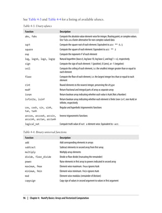
![Function Description
greater, greater_equal,
less, less_equal, equal,
not_equal
Performelement-wisecomparison,yieldingbooleanarray.Equivalenttoinfixoperators
>, >=, <, <=, ==, !=
logical_and,
logical_or, logical_xor
Compute element-wise truth value of logical operation. Equivalent to infix operators &
|, ^
Data Processing Using Arrays
Using NumPy arrays enables you to express many kinds of data processing tasks as
concise array expressions that might otherwise require writing loops. This practice of
replacing explicit loops with array expressions is commonly referred to as vectoriza-
tion. In general, vectorized array operations will often be one or two (or more) orders
of magnitude faster than their pure Python equivalents, with the biggest impact in any
kind of numerical computations. Later, in Chapter 12, I will explain broadcasting, a
powerful method for vectorizing computations.
As a simple example, suppose we wished to evaluate the function sqrt(x^2 + y^2)
across a regular grid of values. The np.meshgrid function takes two 1D arrays and pro-
duces two 2D matrices corresponding to all pairs of (x, y) in the two arrays:
In [130]: points = np.arange(-5, 5, 0.01) # 1000 equally spaced points
In [131]: xs, ys = np.meshgrid(points, points)
In [132]: ys
Out[132]:
array([[-5. , -5. , -5. , ..., -5. , -5. , -5. ],
[-4.99, -4.99, -4.99, ..., -4.99, -4.99, -4.99],
[-4.98, -4.98, -4.98, ..., -4.98, -4.98, -4.98],
...,
[ 4.97, 4.97, 4.97, ..., 4.97, 4.97, 4.97],
[ 4.98, 4.98, 4.98, ..., 4.98, 4.98, 4.98],
[ 4.99, 4.99, 4.99, ..., 4.99, 4.99, 4.99]])
Now, evaluating the function is a simple matter of writing the same expression you
would write with two points:
In [134]: import matplotlib.pyplot as plt
In [135]: z = np.sqrt(xs ** 2 + ys ** 2)
In [136]: z
Out[136]:
array([[ 7.0711, 7.064 , 7.0569, ..., 7.0499, 7.0569, 7.064 ],
[ 7.064 , 7.0569, 7.0499, ..., 7.0428, 7.0499, 7.0569],
[ 7.0569, 7.0499, 7.0428, ..., 7.0357, 7.0428, 7.0499],
...,
[ 7.0499, 7.0428, 7.0357, ..., 7.0286, 7.0357, 7.0428],
[ 7.0569, 7.0499, 7.0428, ..., 7.0357, 7.0428, 7.0499],
[ 7.064 , 7.0569, 7.0499, ..., 7.0428, 7.0499, 7.0569]])
Data Processing Using Arrays | 97](https://image.slidesharecdn.com/wesmckinney-pythonfordataanalysis-oreillymedia2012-221114102054-a802e8f3/85/Wes-McKinney-Python-for-Data-Analysis-O-Reilly-Media-2012-pdf-113-320.jpg)
![In [137]: plt.imshow(z, cmap=plt.cm.gray); plt.colorbar()
Out[137]: <matplotlib.colorbar.Colorbar instance at 0x4e46d40>
In [138]: plt.title("Image plot of $sqrt{x^2 + y^2}$ for a grid of values")
Out[138]: <matplotlib.text.Text at 0x4565790>
See Figure 4-3. Here I used the matplotlib function imshow to create an image plot from
a 2D array of function values.
Figure 4-3. Plot of function evaluated on grid
Expressing Conditional Logic as Array Operations
The numpy.where function is a vectorized version of the ternary expression x if condi
tion else y. Suppose we had a boolean array and two arrays of values:
In [140]: xarr = np.array([1.1, 1.2, 1.3, 1.4, 1.5])
In [141]: yarr = np.array([2.1, 2.2, 2.3, 2.4, 2.5])
In [142]: cond = np.array([True, False, True, True, False])
Suppose we wanted to take a value from xarr whenever the corresponding value in
cond is True otherwise take the value from yarr. A list comprehension doing this might
look like:
In [143]: result = [(x if c else y)
.....: for x, y, c in zip(xarr, yarr, cond)]
In [144]: result
Out[144]: [1.1000000000000001, 2.2000000000000002, 1.3, 1.3999999999999999, 2.5]
98 | Chapter 4: NumPy Basics: Arrays and Vectorized Computation](https://image.slidesharecdn.com/wesmckinney-pythonfordataanalysis-oreillymedia2012-221114102054-a802e8f3/85/Wes-McKinney-Python-for-Data-Analysis-O-Reilly-Media-2012-pdf-114-320.jpg)
![This has multiple problems. First, it will not be very fast for large arrays (because all
the work is being done in pure Python). Secondly, it will not work with multidimen-
sional arrays. With np.where you can write this very concisely:
In [145]: result = np.where(cond, xarr, yarr)
In [146]: result
Out[146]: array([ 1.1, 2.2, 1.3, 1.4, 2.5])
The second and third arguments to np.where don’t need to be arrays; one or both of
them can be scalars. A typical use of where in data analysis is to produce a new array of
values based on another array. Suppose you had a matrix of randomly generated data
and you wanted to replace all positive values with 2 and all negative values with -2.
This is very easy to do with np.where:
In [147]: arr = randn(4, 4)
In [148]: arr
Out[148]:
array([[ 0.6372, 2.2043, 1.7904, 0.0752],
[-1.5926, -1.1536, 0.4413, 0.3483],
[-0.1798, 0.3299, 0.7827, -0.7585],
[ 0.5857, 0.1619, 1.3583, -1.3865]])
In [149]: np.where(arr > 0, 2, -2)
Out[149]:
array([[ 2, 2, 2, 2],
[-2, -2, 2, 2],
[-2, 2, 2, -2],
[ 2, 2, 2, -2]])
In [150]: np.where(arr > 0, 2, arr) # set only positive values to 2
Out[150]:
array([[ 2. , 2. , 2. , 2. ],
[-1.5926, -1.1536, 2. , 2. ],
[-0.1798, 2. , 2. , -0.7585],
[ 2. , 2. , 2. , -1.3865]])
The arrays passed to where can be more than just equal sizes array or scalers.
With some cleverness you can use where to express more complicated logic; consider
this example where I have two boolean arrays, cond1 and cond2, and wish to assign a
different value for each of the 4 possible pairs of boolean values:
result = []
for i in range(n):
if cond1[i] and cond2[i]:
result.append(0)
elif cond1[i]:
result.append(1)
elif cond2[i]:
result.append(2)
else:
result.append(3)
Data Processing Using Arrays | 99](https://image.slidesharecdn.com/wesmckinney-pythonfordataanalysis-oreillymedia2012-221114102054-a802e8f3/85/Wes-McKinney-Python-for-Data-Analysis-O-Reilly-Media-2012-pdf-115-320.jpg)
![While perhaps not immediately obvious, this for loop can be converted into a nested
where expression:
np.where(cond1 & cond2, 0,
np.where(cond1, 1,
np.where(cond2, 2, 3)))
In this particular example, we can also take advantage of the fact that boolean values
are treated as 0 or 1 in calculations, so this could alternatively be expressed (though a
bit more cryptically) as an arithmetic operation:
result = 1 * cond1 + 2 * cond2 + 3 * -(cond1 | cond2)
Mathematical and Statistical Methods
A set of mathematical functions which compute statistics about an entire array or about
the data along an axis are accessible as array methods. Aggregations (often called
reductions) like sum, mean, and standard deviation std can either be used by calling the
array instance method or using the top level NumPy function:
In [151]: arr = np.random.randn(5, 4) # normally-distributed data
In [152]: arr.mean()
Out[152]: 0.062814911084854597
In [153]: np.mean(arr)
Out[153]: 0.062814911084854597
In [154]: arr.sum()
Out[154]: 1.2562982216970919
Functionslikemean andsum takeanoptionalaxis argumentwhichcomputesthestatistic
over the given axis, resulting in an array with one fewer dimension:
In [155]: arr.mean(axis=1)
Out[155]: array([-1.2833, 0.2844, 0.6574, 0.6743, -0.0187])
In [156]: arr.sum(0)
Out[156]: array([-3.1003, -1.6189, 1.4044, 4.5712])
Other methods like cumsum and cumprod do not aggregate, instead producing an array
of the intermediate results:
In [157]: arr = np.array([[0, 1, 2], [3, 4, 5], [6, 7, 8]])
In [158]: arr.cumsum(0) In [159]: arr.cumprod(1)
Out[158]: Out[159]:
array([[ 0, 1, 2], array([[ 0, 0, 0],
[ 3, 5, 7], [ 3, 12, 60],
[ 9, 12, 15]]) [ 6, 42, 336]])
See Table 4-5 for a full listing. We’ll see many examples of these methods in action in
later chapters.
100 | Chapter 4: NumPy Basics: Arrays and Vectorized Computation](https://image.slidesharecdn.com/wesmckinney-pythonfordataanalysis-oreillymedia2012-221114102054-a802e8f3/85/Wes-McKinney-Python-for-Data-Analysis-O-Reilly-Media-2012-pdf-116-320.jpg)
![Table 4-5. Basic array statistical methods
Method Description
sum Sum of all the elements in the array or along an axis. Zero-length arrays have sum 0.
mean Arithmetic mean. Zero-length arrays have NaN mean.
std, var Standarddeviationandvariance,respectively,withoptionaldegreesoffreedomadjust-
ment (default denominator n).
min, max Minimum and maximum.
argmin, argmax Indices of minimum and maximum elements, respectively.
cumsum Cumulative sum of elements starting from 0
cumprod Cumulative product of elements starting from 1
Methods for Boolean Arrays
Boolean values are coerced to 1 (True) and 0 (False) in the above methods. Thus, sum
is often used as a means of counting True values in a boolean array:
In [160]: arr = randn(100)
In [161]: (arr > 0).sum() # Number of positive values
Out[161]: 44
There are two additional methods, any and all, useful especially for boolean arrays.
any tests whether one or more values in an array is True, while all checks if every value
is True:
In [162]: bools = np.array([False, False, True, False])
In [163]: bools.any()
Out[163]: True
In [164]: bools.all()
Out[164]: False
These methods also work with non-boolean arrays, where non-zero elements evaluate
to True.
Sorting
Like Python’s built-in list type, NumPy arrays can be sorted in-place using the sort
method:
In [165]: arr = randn(8)
In [166]: arr
Out[166]:
array([ 0.6903, 0.4678, 0.0968, -0.1349, 0.9879, 0.0185, -1.3147,
-0.5425])
In [167]: arr.sort()
Data Processing Using Arrays | 101](https://image.slidesharecdn.com/wesmckinney-pythonfordataanalysis-oreillymedia2012-221114102054-a802e8f3/85/Wes-McKinney-Python-for-Data-Analysis-O-Reilly-Media-2012-pdf-117-320.jpg)
![In [168]: arr
Out[168]:
array([-1.3147, -0.5425, -0.1349, 0.0185, 0.0968, 0.4678, 0.6903,
0.9879])
Multidimensional arrays can have each 1D section of values sorted in-place along an
axis by passing the axis number to sort:
In [169]: arr = randn(5, 3)
In [170]: arr
Out[170]:
array([[-0.7139, -1.6331, -0.4959],
[ 0.8236, -1.3132, -0.1935],
[-1.6748, 3.0336, -0.863 ],
[-0.3161, 0.5362, -2.468 ],
[ 0.9058, 1.1184, -1.0516]])
In [171]: arr.sort(1)
In [172]: arr
Out[172]:
array([[-1.6331, -0.7139, -0.4959],
[-1.3132, -0.1935, 0.8236],
[-1.6748, -0.863 , 3.0336],
[-2.468 , -0.3161, 0.5362],
[-1.0516, 0.9058, 1.1184]])
The top level method np.sort returns a sorted copy of an array instead of modifying
the array in place. A quick-and-dirty way to compute the quantiles of an array is to sort
it and select the value at a particular rank:
In [173]: large_arr = randn(1000)
In [174]: large_arr.sort()
In [175]: large_arr[int(0.05 * len(large_arr))] # 5% quantile
Out[175]: -1.5791023260896004
For more details on using NumPy’s sorting methods, and more advanced techniques
like indirect sorts, see Chapter 12. Several other kinds of data manipulations related to
sorting (for example, sorting a table of data by one or more columns) are also to be
found in pandas.
Unique and Other Set Logic
NumPy has some basic set operations for one-dimensional ndarrays. Probably the most
commonly used one is np.unique, which returns the sorted unique values in an array:
In [176]: names = np.array(['Bob', 'Joe', 'Will', 'Bob', 'Will', 'Joe', 'Joe'])
In [177]: np.unique(names)
Out[177]:
102 | Chapter 4: NumPy Basics: Arrays and Vectorized Computation](https://image.slidesharecdn.com/wesmckinney-pythonfordataanalysis-oreillymedia2012-221114102054-a802e8f3/85/Wes-McKinney-Python-for-Data-Analysis-O-Reilly-Media-2012-pdf-118-320.jpg)
![array(['Bob', 'Joe', 'Will'],
dtype='|S4')
In [178]: ints = np.array([3, 3, 3, 2, 2, 1, 1, 4, 4])
In [179]: np.unique(ints)
Out[179]: array([1, 2, 3, 4])
Contrast np.unique with the pure Python alternative:
In [180]: sorted(set(names))
Out[180]: ['Bob', 'Joe', 'Will']
Another function, np.in1d, tests membership of the values in one array in another,
returning a boolean array:
In [181]: values = np.array([6, 0, 0, 3, 2, 5, 6])
In [182]: np.in1d(values, [2, 3, 6])
Out[182]: array([ True, False, False, True, True, False, True], dtype=bool)
See Table 4-6 for a listing of set functions in NumPy.
Table 4-6. Array set operations
Method Description
unique(x) Compute the sorted, unique elements in x
intersect1d(x, y) Compute the sorted, common elements in x and y
union1d(x, y) Compute the sorted union of elements
in1d(x, y) Compute a boolean array indicating whether each element of x is contained in y
setdiff1d(x, y) Set difference, elements in x that are not in y
setxor1d(x, y) Set symmetric differences; elements that are in either of the arrays, but not both
File Input and Output with Arrays
NumPy is able to save and load data to and from disk either in text or binary format.
In later chapters you will learn about tools in pandas for reading tabular data into
memory.
Storing Arrays on Disk in Binary Format
np.save and np.load are the two workhorse functions for efficiently saving and loading
array data on disk. Arrays are saved by default in an uncompressed raw binary format
with file extension .npy.
In [183]: arr = np.arange(10)
In [184]: np.save('some_array', arr)
File Input and Output with Arrays | 103](https://image.slidesharecdn.com/wesmckinney-pythonfordataanalysis-oreillymedia2012-221114102054-a802e8f3/85/Wes-McKinney-Python-for-Data-Analysis-O-Reilly-Media-2012-pdf-119-320.jpg)
![If the file path does not already end in .npy, the extension will be appended. The array
on disk can then be loaded using np.load:
In [185]: np.load('some_array.npy')
Out[185]: array([0, 1, 2, 3, 4, 5, 6, 7, 8, 9])
You save multiple arrays in a zip archive using np.savez and passing the arrays as key-
word arguments:
In [186]: np.savez('array_archive.npz', a=arr, b=arr)
When loading an .npz file, you get back a dict-like object which loads the individual
arrays lazily:
In [187]: arch = np.load('array_archive.npz')
In [188]: arch['b']
Out[188]: array([0, 1, 2, 3, 4, 5, 6, 7, 8, 9])
Saving and Loading Text Files
Loading text from files is a fairly standard task. The landscape of file reading and writing
functions in Python can be a bit confusing for a newcomer, so I will focus mainly on
the read_csv and read_table functions in pandas. It will at times be useful to load data
into vanilla NumPy arrays using np.loadtxt or the more specialized np.genfromtxt.
These functions have many options allowing you to specify different delimiters, con-
verter functions for certain columns, skipping rows, and other things. Take a simple
case of a comma-separated file (CSV) like this:
In [191]: !cat array_ex.txt
0.580052,0.186730,1.040717,1.134411
0.194163,-0.636917,-0.938659,0.124094
-0.126410,0.268607,-0.695724,0.047428
-1.484413,0.004176,-0.744203,0.005487
2.302869,0.200131,1.670238,-1.881090
-0.193230,1.047233,0.482803,0.960334
This can be loaded into a 2D array like so:
In [192]: arr = np.loadtxt('array_ex.txt', delimiter=',')
In [193]: arr
Out[193]:
array([[ 0.5801, 0.1867, 1.0407, 1.1344],
[ 0.1942, -0.6369, -0.9387, 0.1241],
[-0.1264, 0.2686, -0.6957, 0.0474],
[-1.4844, 0.0042, -0.7442, 0.0055],
[ 2.3029, 0.2001, 1.6702, -1.8811],
[-0.1932, 1.0472, 0.4828, 0.9603]])
np.savetxt performs the inverse operation: writing an array to a delimited text file.
genfromtxt is similar to loadtxt but is geared for structured arrays and missing data
handling; see Chapter 12 for more on structured arrays.
104 | Chapter 4: NumPy Basics: Arrays and Vectorized Computation](https://image.slidesharecdn.com/wesmckinney-pythonfordataanalysis-oreillymedia2012-221114102054-a802e8f3/85/Wes-McKinney-Python-for-Data-Analysis-O-Reilly-Media-2012-pdf-120-320.jpg)
![For more on file reading and writing, especially tabular or spreadsheet-
likedata,seethelaterchaptersinvolvingpandasandDataFrameobjects.
Linear Algebra
Linear algebra, like matrix multiplication, decompositions, determinants, and other
square matrix math, is an important part of any array library. Unlike some languages
like MATLAB, multiplying two two-dimensional arrays with * is an element-wise
product instead of a matrix dot product. As such, there is a function dot, both an array
method, and a function in the numpy namespace, for matrix multiplication:
In [194]: x = np.array([[1., 2., 3.], [4., 5., 6.]])
In [195]: y = np.array([[6., 23.], [-1, 7], [8, 9]])
In [196]: x In [197]: y
Out[196]: Out[197]:
array([[ 1., 2., 3.], array([[ 6., 23.],
[ 4., 5., 6.]]) [ -1., 7.],
[ 8., 9.]])
In [198]: x.dot(y) # equivalently np.dot(x, y)
Out[198]:
array([[ 28., 64.],
[ 67., 181.]])
A matrix product between a 2D array and a suitably sized 1D array results in a 1D array:
In [199]: np.dot(x, np.ones(3))
Out[199]: array([ 6., 15.])
numpy.linalg has a standard set of matrix decompositions and things like inverse and
determinant. These are implemented under the hood using the same industry-standard
Fortran libraries used in other languages like MATLAB and R, such as like BLAS, LA-
PACK, or possibly (depending on your NumPy build) the Intel MKL:
In [201]: from numpy.linalg import inv, qr
In [202]: X = randn(5, 5)
In [203]: mat = X.T.dot(X)
In [204]: inv(mat)
Out[204]:
array([[ 3.0361, -0.1808, -0.6878, -2.8285, -1.1911],
[-0.1808, 0.5035, 0.1215, 0.6702, 0.0956],
[-0.6878, 0.1215, 0.2904, 0.8081, 0.3049],
[-2.8285, 0.6702, 0.8081, 3.4152, 1.1557],
[-1.1911, 0.0956, 0.3049, 1.1557, 0.6051]])
In [205]: mat.dot(inv(mat))
Linear Algebra | 105](https://image.slidesharecdn.com/wesmckinney-pythonfordataanalysis-oreillymedia2012-221114102054-a802e8f3/85/Wes-McKinney-Python-for-Data-Analysis-O-Reilly-Media-2012-pdf-121-320.jpg)
![Out[205]:
array([[ 1., 0., 0., 0., -0.],
[ 0., 1., -0., 0., 0.],
[ 0., -0., 1., 0., 0.],
[ 0., -0., -0., 1., -0.],
[ 0., 0., 0., 0., 1.]])
In [206]: q, r = qr(mat)
In [207]: r
Out[207]:
array([[ -6.9271, 7.389 , 6.1227, -7.1163, -4.9215],
[ 0. , -3.9735, -0.8671, 2.9747, -5.7402],
[ 0. , 0. , -10.2681, 1.8909, 1.6079],
[ 0. , 0. , 0. , -1.2996, 3.3577],
[ 0. , 0. , 0. , 0. , 0.5571]])
See Table 4-7 for a list of some of the most commonly-used linear algebra functions.
The scientific Python community is hopeful that there may be a matrix
multiplication infix operator implemented someday, providing syntac-
tically nicer alternative to using np.dot. But for now this is the way.
Table 4-7. Commonly-used numpy.linalg functions
Function Description
diag Returnthediagonal(oroff-diagonal)elementsofasquarematrixasa1Darray,orconverta1Darrayintoasquare
matrix with zeros on the off-diagonal
dot Matrix multiplication
trace Compute the sum of the diagonal elements
det Compute the matrix determinant
eig Compute the eigenvalues and eigenvectors of a square matrix
inv Compute the inverse of a square matrix
pinv Compute the Moore-Penrose pseudo-inverse inverse of a square matrix
qr Compute the QR decomposition
svd Compute the singular value decomposition (SVD)
solve Solve the linear system Ax = b for x, where A is a square matrix
lstsq Compute the least-squares solution to y = Xb
Random Number Generation
The numpy.random module supplements the built-in Python random with functions for
efficiently generating whole arrays of sample values from many kinds of probability
106 | Chapter 4: NumPy Basics: Arrays and Vectorized Computation](https://image.slidesharecdn.com/wesmckinney-pythonfordataanalysis-oreillymedia2012-221114102054-a802e8f3/85/Wes-McKinney-Python-for-Data-Analysis-O-Reilly-Media-2012-pdf-122-320.jpg)
![distributions. For example, you can get a 4 by 4 array of samples from the standard
normal distribution using normal:
In [208]: samples = np.random.normal(size=(4, 4))
In [209]: samples
Out[209]:
array([[ 0.1241, 0.3026, 0.5238, 0.0009],
[ 1.3438, -0.7135, -0.8312, -2.3702],
[-1.8608, -0.8608, 0.5601, -1.2659],
[ 0.1198, -1.0635, 0.3329, -2.3594]])
Python’s built-in random module, by contrast, only samples one value at a time. As you
can see from this benchmark, numpy.random is well over an order of magnitude faster
for generating very large samples:
In [210]: from random import normalvariate
In [211]: N = 1000000
In [212]: %timeit samples = [normalvariate(0, 1) for _ in xrange(N)]
1 loops, best of 3: 1.33 s per loop
In [213]: %timeit np.random.normal(size=N)
10 loops, best of 3: 57.7 ms per loop
See table Table 4-8 for a partial list of functions available in numpy.random. I’ll give some
examples of leveraging these functions’ ability to generate large arrays of samples all at
once in the next section.
Table 4-8. Partial list of numpy.random functions
Function Description
seed Seed the random number generator
permutation Return a random permutation of a sequence, or return a permuted range
shuffle Randomly permute a sequence in place
rand Draw samples from a uniform distribution
randint Draw random integers from a given low-to-high range
randn Draw samples from a normal distribution with mean 0 and standard deviation 1 (MATLAB-like interface)
binomial Draw samples a binomial distribution
normal Draw samples from a normal (Gaussian) distribution
beta Draw samples from a beta distribution
chisquare Draw samples from a chi-square distribution
gamma Draw samples from a gamma distribution
uniform Draw samples from a uniform [0, 1) distribution
Random Number Generation | 107](https://image.slidesharecdn.com/wesmckinney-pythonfordataanalysis-oreillymedia2012-221114102054-a802e8f3/85/Wes-McKinney-Python-for-Data-Analysis-O-Reilly-Media-2012-pdf-123-320.jpg)
![Example: Random Walks
An illustrative application of utilizing array operations is in the simulation of random
walks. Let’s first consider a simple random walk starting at 0 with steps of 1 and -1
occurring with equal probability. A pure Python way to implement a single random
walk with 1,000 steps using the built-in random module:
import random
position = 0
walk = [position]
steps = 1000
for i in xrange(steps):
step = 1 if random.randint(0, 1) else -1
position += step
walk.append(position)
See Figure 4-4 for an example plot of the first 100 values on one of these random walks.
Figure 4-4. A simple random walk
You might make the observation that walk is simply the cumulative sum of the random
steps and could be evaluated as an array expression. Thus, I use the np.random module
to draw 1,000 coin flips at once, set these to 1 and -1, and compute the cumulative sum:
In [215]: nsteps = 1000
In [216]: draws = np.random.randint(0, 2, size=nsteps)
In [217]: steps = np.where(draws > 0, 1, -1)
In [218]: walk = steps.cumsum()
108 | Chapter 4: NumPy Basics: Arrays and Vectorized Computation](https://image.slidesharecdn.com/wesmckinney-pythonfordataanalysis-oreillymedia2012-221114102054-a802e8f3/85/Wes-McKinney-Python-for-Data-Analysis-O-Reilly-Media-2012-pdf-124-320.jpg)
![From this we can begin to extract statistics like the minimum and maximum value along
the walk’s trajectory:
In [219]: walk.min() In [220]: walk.max()
Out[219]: -3 Out[220]: 31
A more complicated statistic is the first crossing time, the step at which the random
walk reaches a particular value. Here we might want to know how long it took the
random walk to get at least 10 steps away from the origin 0 in either direction.
np.abs(walk) >= 10 gives us a boolean array indicating where the walk has reached or
exceeded 10, but we want the index of the first 10 or -10. Turns out this can be com-
puted using argmax, which returns the first index of the maximum value in the boolean
array (True is the maximum value):
In [221]: (np.abs(walk) >= 10).argmax()
Out[221]: 37
Note that using argmax here is not always efficient because it always makes a full scan
of the array. In this special case once a True is observed we know it to be the maximum
value.
Simulating Many Random Walks at Once
If your goal was to simulate many random walks, say 5,000 of them, you can generate
all of the random walks with minor modifications to the above code. The numpy.ran
dom functions if passed a 2-tuple will generate a 2D array of draws, and we can compute
the cumulative sum across the rows to compute all 5,000 random walks in one shot:
In [222]: nwalks = 5000
In [223]: nsteps = 1000
In [224]: draws = np.random.randint(0, 2, size=(nwalks, nsteps)) # 0 or 1
In [225]: steps = np.where(draws > 0, 1, -1)
In [226]: walks = steps.cumsum(1)
In [227]: walks
Out[227]:
array([[ 1, 0, 1, ..., 8, 7, 8],
[ 1, 0, -1, ..., 34, 33, 32],
[ 1, 0, -1, ..., 4, 5, 4],
...,
[ 1, 2, 1, ..., 24, 25, 26],
[ 1, 2, 3, ..., 14, 13, 14],
[ -1, -2, -3, ..., -24, -23, -22]])
Now, we can compute the maximum and minimum values obtained over all of the
walks:
In [228]: walks.max() In [229]: walks.min()
Out[228]: 138 Out[229]: -133
Example: Random Walks | 109](https://image.slidesharecdn.com/wesmckinney-pythonfordataanalysis-oreillymedia2012-221114102054-a802e8f3/85/Wes-McKinney-Python-for-Data-Analysis-O-Reilly-Media-2012-pdf-125-320.jpg)
![Out of these walks, let’s compute the minimum crossing time to 30 or -30. This is
slightly tricky because not all 5,000 of them reach 30. We can check this using the
any method:
In [230]: hits30 = (np.abs(walks) >= 30).any(1)
In [231]: hits30
Out[231]: array([False, True, False, ..., False, True, False], dtype=bool)
In [232]: hits30.sum() # Number that hit 30 or -30
Out[232]: 3410
We can use this boolean array to select out the rows of walks that actually cross the
absolute 30 level and call argmax across axis 1 to get the crossing times:
In [233]: crossing_times = (np.abs(walks[hits30]) >= 30).argmax(1)
In [234]: crossing_times.mean()
Out[234]: 498.88973607038122
Feel free to experiment with other distributions for the steps other than equal sized
coin flips. You need only use a different random number generation function, like
normal to generate normally distributed steps with some mean and standard deviation:
In [235]: steps = np.random.normal(loc=0, scale=0.25,
.....: size=(nwalks, nsteps))
110 | Chapter 4: NumPy Basics: Arrays and Vectorized Computation](https://image.slidesharecdn.com/wesmckinney-pythonfordataanalysis-oreillymedia2012-221114102054-a802e8f3/85/Wes-McKinney-Python-for-Data-Analysis-O-Reilly-Media-2012-pdf-126-320.jpg)
![In [1]: from pandas import Series, DataFrame
In [2]: import pandas as pd
Thus, whenever you see pd. in code, it’s referring to pandas. Series and DataFrame are
used so much that I find it easier to import them into the local namespace.
Introduction to pandas Data Structures
To get started with pandas, you will need to get comfortable with its two workhorse
data structures: Series and DataFrame. While they are not a universal solution for every
problem, they provide a solid, easy-to-use basis for most applications.
Series
A Series is a one-dimensional array-like object containing an array of data (of any
NumPy data type) and an associated array of data labels, called its index. The simplest
Series is formed from only an array of data:
In [4]: obj = Series([4, 7, -5, 3])
In [5]: obj
Out[5]:
0 4
1 7
2 -5
3 3
The string representation of a Series displayed interactively shows the index on the left
and the values on the right. Since we did not specify an index for the data, a default
one consisting of the integers 0 through N - 1 (where N is the length of the data) is
created. You can get the array representation and index object of the Series via its values
and index attributes, respectively:
In [6]: obj.values
Out[6]: array([ 4, 7, -5, 3])
In [7]: obj.index
Out[7]: Int64Index([0, 1, 2, 3])
Often it will be desirable to create a Series with an index identifying each data point:
In [8]: obj2 = Series([4, 7, -5, 3], index=['d', 'b', 'a', 'c'])
In [9]: obj2
Out[9]:
d 4
b 7
a -5
c 3
112 | Chapter 5: Getting Started with pandas](https://image.slidesharecdn.com/wesmckinney-pythonfordataanalysis-oreillymedia2012-221114102054-a802e8f3/85/Wes-McKinney-Python-for-Data-Analysis-O-Reilly-Media-2012-pdf-128-320.jpg)
![In [10]: obj2.index
Out[10]: Index([d, b, a, c], dtype=object)
Compared with a regular NumPy array, you can use values in the index when selecting
single values or a set of values:
In [11]: obj2['a']
Out[11]: -5
In [12]: obj2['d'] = 6
In [13]: obj2[['c', 'a', 'd']]
Out[13]:
c 3
a -5
d 6
NumPy array operations, such as filtering with a boolean array, scalar multiplication,
or applying math functions, will preserve the index-value link:
In [14]: obj2
Out[14]:
d 6
b 7
a -5
c 3
In [15]: obj2[obj2 > 0] In [16]: obj2 * 2 In [17]: np.exp(obj2)
Out[15]: Out[16]: Out[17]:
d 6 d 12 d 403.428793
b 7 b 14 b 1096.633158
c 3 a -10 a 0.006738
c 6 c 20.085537
Another way to think about a Series is as a fixed-length, ordered dict, as it is a mapping
of index values to data values. It can be substituted into many functions that expect a
dict:
In [18]: 'b' in obj2
Out[18]: True
In [19]: 'e' in obj2
Out[19]: False
Should you have data contained in a Python dict, you can create a Series from it by
passing the dict:
In [20]: sdata = {'Ohio': 35000, 'Texas': 71000, 'Oregon': 16000, 'Utah': 5000}
In [21]: obj3 = Series(sdata)
In [22]: obj3
Out[22]:
Ohio 35000
Oregon 16000
Introduction to pandas Data Structures | 113](https://image.slidesharecdn.com/wesmckinney-pythonfordataanalysis-oreillymedia2012-221114102054-a802e8f3/85/Wes-McKinney-Python-for-Data-Analysis-O-Reilly-Media-2012-pdf-129-320.jpg)
![Texas 71000
Utah 5000
When only passing a dict, the index in the resulting Series will have the dict’s keys in
sorted order.
In [23]: states = ['California', 'Ohio', 'Oregon', 'Texas']
In [24]: obj4 = Series(sdata, index=states)
In [25]: obj4
Out[25]:
California NaN
Ohio 35000
Oregon 16000
Texas 71000
In this case, 3 values found in sdata were placed in the appropriate locations, but since
no value for 'California' was found, it appears as NaN (not a number) which is con-
sidered in pandas to mark missing or NA values. I will use the terms “missing” or “NA”
to refer to missing data. The isnull and notnull functions in pandas should be used to
detect missing data:
In [26]: pd.isnull(obj4) In [27]: pd.notnull(obj4)
Out[26]: Out[27]:
California True California False
Ohio False Ohio True
Oregon False Oregon True
Texas False Texas True
Series also has these as instance methods:
In [28]: obj4.isnull()
Out[28]:
California True
Ohio False
Oregon False
Texas False
I discuss working with missing data in more detail later in this chapter.
A critical Series feature for many applications is that it automatically aligns differently-
indexed data in arithmetic operations:
In [29]: obj3 In [30]: obj4
Out[29]: Out[30]:
Ohio 35000 California NaN
Oregon 16000 Ohio 35000
Texas 71000 Oregon 16000
Utah 5000 Texas 71000
In [31]: obj3 + obj4
Out[31]:
California NaN
Ohio 70000
Oregon 32000
114 | Chapter 5: Getting Started with pandas](https://image.slidesharecdn.com/wesmckinney-pythonfordataanalysis-oreillymedia2012-221114102054-a802e8f3/85/Wes-McKinney-Python-for-Data-Analysis-O-Reilly-Media-2012-pdf-130-320.jpg)
![Texas 142000
Utah NaN
Data alignment features are addressed as a separate topic.
Both the Series object itself and its index have a name attribute, which integrates with
other key areas of pandas functionality:
In [32]: obj4.name = 'population'
In [33]: obj4.index.name = 'state'
In [34]: obj4
Out[34]:
state
California NaN
Ohio 35000
Oregon 16000
Texas 71000
Name: population
A Series’s index can be altered in place by assignment:
In [35]: obj.index = ['Bob', 'Steve', 'Jeff', 'Ryan']
In [36]: obj
Out[36]:
Bob 4
Steve 7
Jeff -5
Ryan 3
DataFrame
A DataFrame represents a tabular, spreadsheet-like data structure containing an or-
dered collection of columns, each of which can be a different value type (numeric,
string, boolean, etc.). The DataFrame has both a row and column index; it can be
thought of as a dict of Series (one for all sharing the same index). Compared with other
such DataFrame-like structures you may have used before (like R’s data.frame), row-
oriented and column-oriented operations in DataFrame are treated roughly symmet-
rically. Under the hood, the data is stored as one or more two-dimensional blocks rather
than a list, dict, or some other collection of one-dimensional arrays. The exact details
of DataFrame’s internals are far outside the scope of this book.
While DataFrame stores the data internally in a two-dimensional for-
mat, you can easily represent much higher-dimensional data in a tabular
format using hierarchical indexing, a subject of a later section and a key
ingredient in many of the more advanced data-handling features in pan-
das.
Introduction to pandas Data Structures | 115](https://image.slidesharecdn.com/wesmckinney-pythonfordataanalysis-oreillymedia2012-221114102054-a802e8f3/85/Wes-McKinney-Python-for-Data-Analysis-O-Reilly-Media-2012-pdf-131-320.jpg)
![There are numerous ways to construct a DataFrame, though one of the most common
is from a dict of equal-length lists or NumPy arrays
data = {'state': ['Ohio', 'Ohio', 'Ohio', 'Nevada', 'Nevada'],
'year': [2000, 2001, 2002, 2001, 2002],
'pop': [1.5, 1.7, 3.6, 2.4, 2.9]}
frame = DataFrame(data)
The resulting DataFrame will have its index assigned automatically as with Series, and
the columns are placed in sorted order:
In [38]: frame
Out[38]:
pop state year
0 1.5 Ohio 2000
1 1.7 Ohio 2001
2 3.6 Ohio 2002
3 2.4 Nevada 2001
4 2.9 Nevada 2002
If you specify a sequence of columns, the DataFrame’s columns will be exactly what
you pass:
In [39]: DataFrame(data, columns=['year', 'state', 'pop'])
Out[39]:
year state pop
0 2000 Ohio 1.5
1 2001 Ohio 1.7
2 2002 Ohio 3.6
3 2001 Nevada 2.4
4 2002 Nevada 2.9
As with Series, if you pass a column that isn’t contained in data, it will appear with NA
values in the result:
In [40]: frame2 = DataFrame(data, columns=['year', 'state', 'pop', 'debt'],
....: index=['one', 'two', 'three', 'four', 'five'])
In [41]: frame2
Out[41]:
year state pop debt
one 2000 Ohio 1.5 NaN
two 2001 Ohio 1.7 NaN
three 2002 Ohio 3.6 NaN
four 2001 Nevada 2.4 NaN
five 2002 Nevada 2.9 NaN
In [42]: frame2.columns
Out[42]: Index([year, state, pop, debt], dtype=object)
A column in a DataFrame can be retrieved as a Series either by dict-like notation or by
attribute:
In [43]: frame2['state'] In [44]: frame2.year
Out[43]: Out[44]:
one Ohio one 2000
116 | Chapter 5: Getting Started with pandas](https://image.slidesharecdn.com/wesmckinney-pythonfordataanalysis-oreillymedia2012-221114102054-a802e8f3/85/Wes-McKinney-Python-for-Data-Analysis-O-Reilly-Media-2012-pdf-132-320.jpg)
![two Ohio two 2001
three Ohio three 2002
four Nevada four 2001
five Nevada five 2002
Name: state Name: year
Note that the returned Series have the same index as the DataFrame, and their name
attribute has been appropriately set.
Rows can also be retrieved by position or name by a couple of methods, such as the
ix indexing field (much more on this later):
In [45]: frame2.ix['three']
Out[45]:
year 2002
state Ohio
pop 3.6
debt NaN
Name: three
Columns can be modified by assignment. For example, the empty 'debt' column could
be assigned a scalar value or an array of values:
In [46]: frame2['debt'] = 16.5
In [47]: frame2
Out[47]:
year state pop debt
one 2000 Ohio 1.5 16.5
two 2001 Ohio 1.7 16.5
three 2002 Ohio 3.6 16.5
four 2001 Nevada 2.4 16.5
five 2002 Nevada 2.9 16.5
In [48]: frame2['debt'] = np.arange(5.)
In [49]: frame2
Out[49]:
year state pop debt
one 2000 Ohio 1.5 0
two 2001 Ohio 1.7 1
three 2002 Ohio 3.6 2
four 2001 Nevada 2.4 3
five 2002 Nevada 2.9 4
When assigning lists or arrays to a column, the value’s length must match the length
of the DataFrame. If you assign a Series, it will be instead conformed exactly to the
DataFrame’s index, inserting missing values in any holes:
In [50]: val = Series([-1.2, -1.5, -1.7], index=['two', 'four', 'five'])
In [51]: frame2['debt'] = val
In [52]: frame2
Out[52]:
year state pop debt
Introduction to pandas Data Structures | 117](https://image.slidesharecdn.com/wesmckinney-pythonfordataanalysis-oreillymedia2012-221114102054-a802e8f3/85/Wes-McKinney-Python-for-Data-Analysis-O-Reilly-Media-2012-pdf-133-320.jpg)
![one 2000 Ohio 1.5 NaN
two 2001 Ohio 1.7 -1.2
three 2002 Ohio 3.6 NaN
four 2001 Nevada 2.4 -1.5
five 2002 Nevada 2.9 -1.7
Assigning a column that doesn’t exist will create a new column. The del keyword will
delete columns as with a dict:
In [53]: frame2['eastern'] = frame2.state == 'Ohio'
In [54]: frame2
Out[54]:
year state pop debt eastern
one 2000 Ohio 1.5 NaN True
two 2001 Ohio 1.7 -1.2 True
three 2002 Ohio 3.6 NaN True
four 2001 Nevada 2.4 -1.5 False
five 2002 Nevada 2.9 -1.7 False
In [55]: del frame2['eastern']
In [56]: frame2.columns
Out[56]: Index([year, state, pop, debt], dtype=object)
The column returned when indexing a DataFrame is a view on the un-
derlying data, not a copy. Thus, any in-place modifications to the Series
will be reflected in the DataFrame. The column can be explicitly copied
using the Series’s copy method.
Another common form of data is a nested dict of dicts format:
In [57]: pop = {'Nevada': {2001: 2.4, 2002: 2.9},
....: 'Ohio': {2000: 1.5, 2001: 1.7, 2002: 3.6}}
If passed to DataFrame, it will interpret the outer dict keys as the columns and the inner
keys as the row indices:
In [58]: frame3 = DataFrame(pop)
In [59]: frame3
Out[59]:
Nevada Ohio
2000 NaN 1.5
2001 2.4 1.7
2002 2.9 3.6
Of course you can always transpose the result:
In [60]: frame3.T
Out[60]:
2000 2001 2002
Nevada NaN 2.4 2.9
Ohio 1.5 1.7 3.6
118 | Chapter 5: Getting Started with pandas](https://image.slidesharecdn.com/wesmckinney-pythonfordataanalysis-oreillymedia2012-221114102054-a802e8f3/85/Wes-McKinney-Python-for-Data-Analysis-O-Reilly-Media-2012-pdf-134-320.jpg)
![The keys in the inner dicts are unioned and sorted to form the index in the result. This
isn’t true if an explicit index is specified:
In [61]: DataFrame(pop, index=[2001, 2002, 2003])
Out[61]:
Nevada Ohio
2001 2.4 1.7
2002 2.9 3.6
2003 NaN NaN
Dicts of Series are treated much in the same way:
In [62]: pdata = {'Ohio': frame3['Ohio'][:-1],
....: 'Nevada': frame3['Nevada'][:2]}
In [63]: DataFrame(pdata)
Out[63]:
Nevada Ohio
2000 NaN 1.5
2001 2.4 1.7
For a complete list of things you can pass the DataFrame constructor, see Table 5-1.
If a DataFrame’s index and columns have their name attributes set, these will also be
displayed:
In [64]: frame3.index.name = 'year'; frame3.columns.name = 'state'
In [65]: frame3
Out[65]:
state Nevada Ohio
year
2000 NaN 1.5
2001 2.4 1.7
2002 2.9 3.6
Like Series, the values attribute returns the data contained in the DataFrame as a 2D
ndarray:
In [66]: frame3.values
Out[66]:
array([[ nan, 1.5],
[ 2.4, 1.7],
[ 2.9, 3.6]])
If the DataFrame’s columns are different dtypes, the dtype of the values array will be
chosen to accomodate all of the columns:
In [67]: frame2.values
Out[67]:
array([[2000, Ohio, 1.5, nan],
[2001, Ohio, 1.7, -1.2],
[2002, Ohio, 3.6, nan],
[2001, Nevada, 2.4, -1.5],
[2002, Nevada, 2.9, -1.7]], dtype=object)
Introduction to pandas Data Structures | 119](https://image.slidesharecdn.com/wesmckinney-pythonfordataanalysis-oreillymedia2012-221114102054-a802e8f3/85/Wes-McKinney-Python-for-Data-Analysis-O-Reilly-Media-2012-pdf-135-320.jpg)
![Table 5-1. Possible data inputs to DataFrame constructor
Type Notes
2D ndarray A matrix of data, passing optional row and column labels
dict of arrays, lists, or tuples EachsequencebecomesacolumnintheDataFrame.Allsequencesmustbethesamelength.
NumPy structured/record array Treated as the “dict of arrays” case
dict of Series Each value becomes a column. Indexes from each Series are unioned together to form the
result’s row index if no explicit index is passed.
dict of dicts Each inner dict becomes a column. Keys are unioned to form the row index as in the “dict of
Series” case.
list of dicts or Series EachitembecomesarowintheDataFrame.UnionofdictkeysorSeriesindexesbecomethe
DataFrame’s column labels
List of lists or tuples Treated as the “2D ndarray” case
Another DataFrame The DataFrame’s indexes are used unless different ones are passed
NumPy MaskedArray Likethe“2Dndarray”caseexceptmaskedvaluesbecomeNA/missingintheDataFrameresult
Index Objects
pandas’s Index objects are responsible for holding the axis labels and other metadata
(like the axis name or names). Any array or other sequence of labels used when con-
structing a Series or DataFrame is internally converted to an Index:
In [68]: obj = Series(range(3), index=['a', 'b', 'c'])
In [69]: index = obj.index
In [70]: index
Out[70]: Index([a, b, c], dtype=object)
In [71]: index[1:]
Out[71]: Index([b, c], dtype=object)
Index objects are immutable and thus can’t be modified by the user:
In [72]: index[1] = 'd'
---------------------------------------------------------------------------
Exception Traceback (most recent call last)
<ipython-input-72-676fdeb26a68> in <module>()
----> 1 index[1] = 'd'
/Users/wesm/code/pandas/pandas/core/index.pyc in __setitem__(self, key, value)
302 def __setitem__(self, key, value):
303 """Disable the setting of values."""
--> 304 raise Exception(str(self.__class__) + ' object is immutable')
305
306 def __getitem__(self, key):
Exception: <class 'pandas.core.index.Index'> object is immutable
120 | Chapter 5: Getting Started with pandas](https://image.slidesharecdn.com/wesmckinney-pythonfordataanalysis-oreillymedia2012-221114102054-a802e8f3/85/Wes-McKinney-Python-for-Data-Analysis-O-Reilly-Media-2012-pdf-136-320.jpg)
![Immutability is important so that Index objects can be safely shared among data
structures:
In [73]: index = pd.Index(np.arange(3))
In [74]: obj2 = Series([1.5, -2.5, 0], index=index)
In [75]: obj2.index is index
Out[75]: True
Table 5-2 has a list of built-in Index classes in the library. With some development
effort, Index can even be subclassed to implement specialized axis indexing function-
ality.
Many users will not need to know much about Index objects, but they’re
nonetheless an important part of pandas’s data model.
Table 5-2. Main Index objects in pandas
Class Description
Index The most general Index object, representing axis labels in a NumPy array of Python objects.
Int64Index Specialized Index for integer values.
MultiIndex “Hierarchical” index object representing multiple levels of indexing on a single axis. Can be thought of
as similar to an array of tuples.
DatetimeIndex Stores nanosecond timestamps (represented using NumPy’s datetime64 dtype).
PeriodIndex Specialized Index for Period data (timespans).
In addition to being array-like, an Index also functions as a fixed-size set:
In [76]: frame3
Out[76]:
state Nevada Ohio
year
2000 NaN 1.5
2001 2.4 1.7
2002 2.9 3.6
In [77]: 'Ohio' in frame3.columns
Out[77]: True
In [78]: 2003 in frame3.index
Out[78]: False
Each Index has a number of methods and properties for set logic and answering other
common questions about the data it contains. These are summarized in Table 5-3.
Introduction to pandas Data Structures | 121](https://image.slidesharecdn.com/wesmckinney-pythonfordataanalysis-oreillymedia2012-221114102054-a802e8f3/85/Wes-McKinney-Python-for-Data-Analysis-O-Reilly-Media-2012-pdf-137-320.jpg)
![Table 5-3. Index methods and properties
Method Description
append Concatenate with additional Index objects, producing a new Index
diff Compute set difference as an Index
intersection Compute set intersection
union Compute set union
isin Compute boolean array indicating whether each value is contained in the passed collection
delete Compute new Index with element at index i deleted
drop Compute new index by deleting passed values
insert Compute new Index by inserting element at index i
is_monotonic Returns True if each element is greater than or equal to the previous element
is_unique Returns True if the Index has no duplicate values
unique Compute the array of unique values in the Index
Essential Functionality
In this section, I’ll walk you through the fundamental mechanics of interacting with
the data contained in a Series or DataFrame. Upcoming chapters will delve more deeply
into data analysis and manipulation topics using pandas. This book is not intended to
serve as exhaustive documentation for the pandas library; I instead focus on the most
important features, leaving the less common (that is, more esoteric) things for you to
explore on your own.
Reindexing
A critical method on pandas objects is reindex, which means to create a new object
with the data conformed to a new index. Consider a simple example from above:
In [79]: obj = Series([4.5, 7.2, -5.3, 3.6], index=['d', 'b', 'a', 'c'])
In [80]: obj
Out[80]:
d 4.5
b 7.2
a -5.3
c 3.6
Calling reindex on this Series rearranges the data according to the new index, intro-
ducing missing values if any index values were not already present:
In [81]: obj2 = obj.reindex(['a', 'b', 'c', 'd', 'e'])
In [82]: obj2
Out[82]:
a -5.3
122 | Chapter 5: Getting Started with pandas](https://image.slidesharecdn.com/wesmckinney-pythonfordataanalysis-oreillymedia2012-221114102054-a802e8f3/85/Wes-McKinney-Python-for-Data-Analysis-O-Reilly-Media-2012-pdf-138-320.jpg)
![b 7.2
c 3.6
d 4.5
e NaN
In [83]: obj.reindex(['a', 'b', 'c', 'd', 'e'], fill_value=0)
Out[83]:
a -5.3
b 7.2
c 3.6
d 4.5
e 0.0
For ordered data like time series, it may be desirable to do some interpolation or filling
of values when reindexing. The method option allows us to do this, using a method such
as ffill which forward fills the values:
In [84]: obj3 = Series(['blue', 'purple', 'yellow'], index=[0, 2, 4])
In [85]: obj3.reindex(range(6), method='ffill')
Out[85]:
0 blue
1 blue
2 purple
3 purple
4 yellow
5 yellow
Table 5-4 lists available method options. At this time, interpolation more sophisticated
than forward- and backfilling would need to be applied after the fact.
Table 5-4. reindex method (interpolation) options
Argument Description
ffill or pad Fill (or carry) values forward
bfill or backfill Fill (or carry) values backward
With DataFrame, reindex can alter either the (row) index, columns, or both. When
passed just a sequence, the rows are reindexed in the result:
In [86]: frame = DataFrame(np.arange(9).reshape((3, 3)), index=['a', 'c', 'd'],
....: columns=['Ohio', 'Texas', 'California'])
In [87]: frame
Out[87]:
Ohio Texas California
a 0 1 2
c 3 4 5
d 6 7 8
In [88]: frame2 = frame.reindex(['a', 'b', 'c', 'd'])
In [89]: frame2
Out[89]:
Essential Functionality | 123](https://image.slidesharecdn.com/wesmckinney-pythonfordataanalysis-oreillymedia2012-221114102054-a802e8f3/85/Wes-McKinney-Python-for-Data-Analysis-O-Reilly-Media-2012-pdf-139-320.jpg)
![Ohio Texas California
a 0 1 2
b NaN NaN NaN
c 3 4 5
d 6 7 8
The columns can be reindexed using the columns keyword:
In [90]: states = ['Texas', 'Utah', 'California']
In [91]: frame.reindex(columns=states)
Out[91]:
Texas Utah California
a 1 NaN 2
c 4 NaN 5
d 7 NaN 8
Both can be reindexed in one shot, though interpolation will only apply row-wise (axis
0):
In [92]: frame.reindex(index=['a', 'b', 'c', 'd'], method='ffill',
....: columns=states)
Out[92]:
Texas Utah California
a 1 NaN 2
b 1 NaN 2
c 4 NaN 5
d 7 NaN 8
As you’ll see soon, reindexing can be done more succinctly by label-indexing with ix:
In [93]: frame.ix[['a', 'b', 'c', 'd'], states]
Out[93]:
Texas Utah California
a 1 NaN 2
b NaN NaN NaN
c 4 NaN 5
d 7 NaN 8
Table 5-5. reindex function arguments
Argument Description
index New sequence to use as index. Can be Index instance or any other sequence-like Python data structure. An
Index will be used exactly as is without any copying
method Interpolation (fill) method, see Table 5-4 for options.
fill_value Substitute value to use when introducing missing data by reindexing
limit When forward- or backfilling, maximum size gap to fill
level Match simple Index on level of MultiIndex, otherwise select subset of
copy Donotcopyunderlyingdataifnewindexisequivalenttooldindex.True bydefault(i.e.alwayscopydata).
124 | Chapter 5: Getting Started with pandas](https://image.slidesharecdn.com/wesmckinney-pythonfordataanalysis-oreillymedia2012-221114102054-a802e8f3/85/Wes-McKinney-Python-for-Data-Analysis-O-Reilly-Media-2012-pdf-140-320.jpg)
![Dropping entries from an axis
Dropping one or more entries from an axis is easy if you have an index array or list
without those entries. As that can require a bit of munging and set logic, the drop
method will return a new object with the indicated value or values deleted from an axis:
In [94]: obj = Series(np.arange(5.), index=['a', 'b', 'c', 'd', 'e'])
In [95]: new_obj = obj.drop('c')
In [96]: new_obj
Out[96]:
a 0
b 1
d 3
e 4
In [97]: obj.drop(['d', 'c'])
Out[97]:
a 0
b 1
e 4
With DataFrame, index values can be deleted from either axis:
In [98]: data = DataFrame(np.arange(16).reshape((4, 4)),
....: index=['Ohio', 'Colorado', 'Utah', 'New York'],
....: columns=['one', 'two', 'three', 'four'])
In [99]: data.drop(['Colorado', 'Ohio'])
Out[99]:
one two three four
Utah 8 9 10 11
New York 12 13 14 15
In [100]: data.drop('two', axis=1) In [101]: data.drop(['two', 'four'], axis=1)
Out[100]: Out[101]:
one three four one three
Ohio 0 2 3 Ohio 0 2
Colorado 4 6 7 Colorado 4 6
Utah 8 10 11 Utah 8 10
New York 12 14 15 New York 12 14
Indexing, selection, and filtering
Series indexing (obj[...]) works analogously to NumPy array indexing, except you can
use the Series’s index values instead of only integers. Here are some examples this:
In [102]: obj = Series(np.arange(4.), index=['a', 'b', 'c', 'd'])
In [103]: obj['b'] In [104]: obj[1]
Out[103]: 1.0 Out[104]: 1.0
In [105]: obj[2:4] In [106]: obj[['b', 'a', 'd']]
Out[105]: Out[106]:
Essential Functionality | 125](https://image.slidesharecdn.com/wesmckinney-pythonfordataanalysis-oreillymedia2012-221114102054-a802e8f3/85/Wes-McKinney-Python-for-Data-Analysis-O-Reilly-Media-2012-pdf-141-320.jpg)
![c 2 b 1
d 3 a 0
d 3
In [107]: obj[[1, 3]] In [108]: obj[obj < 2]
Out[107]: Out[108]:
b 1 a 0
d 3 b 1
Slicing with labels behaves differently than normal Python slicing in that the endpoint
is inclusive:
In [109]: obj['b':'c']
Out[109]:
b 1
c 2
Setting using these methods works just as you would expect:
In [110]: obj['b':'c'] = 5
In [111]: obj
Out[111]:
a 0
b 5
c 5
d 3
As you’ve seen above, indexing into a DataFrame is for retrieving one or more columns
either with a single value or sequence:
In [112]: data = DataFrame(np.arange(16).reshape((4, 4)),
.....: index=['Ohio', 'Colorado', 'Utah', 'New York'],
.....: columns=['one', 'two', 'three', 'four'])
In [113]: data
Out[113]:
one two three four
Ohio 0 1 2 3
Colorado 4 5 6 7
Utah 8 9 10 11
New York 12 13 14 15
In [114]: data['two'] In [115]: data[['three', 'one']]
Out[114]: Out[115]:
Ohio 1 three one
Colorado 5 Ohio 2 0
Utah 9 Colorado 6 4
New York 13 Utah 10 8
Name: two New York 14 12
Indexing like this has a few special cases. First selecting rows by slicing or a boolean
array:
In [116]: data[:2] In [117]: data[data['three'] > 5]
Out[116]: Out[117]:
one two three four one two three four
126 | Chapter 5: Getting Started with pandas](https://image.slidesharecdn.com/wesmckinney-pythonfordataanalysis-oreillymedia2012-221114102054-a802e8f3/85/Wes-McKinney-Python-for-Data-Analysis-O-Reilly-Media-2012-pdf-142-320.jpg)
![Ohio 0 1 2 3 Colorado 4 5 6 7
Colorado 4 5 6 7 Utah 8 9 10 11
New York 12 13 14 15
This might seem inconsistent to some readers, but this syntax arose out of practicality
and nothing more. Another use case is in indexing with a boolean DataFrame, such as
one produced by a scalar comparison:
In [118]: data < 5
Out[118]:
one two three four
Ohio True True True True
Colorado True False False False
Utah False False False False
New York False False False False
In [119]: data[data < 5] = 0
In [120]: data
Out[120]:
one two three four
Ohio 0 0 0 0
Colorado 0 5 6 7
Utah 8 9 10 11
New York 12 13 14 15
This is intended to make DataFrame syntactically more like an ndarray in this case.
For DataFrame label-indexing on the rows, I introduce the special indexing field ix. It
enables you to select a subset of the rows and columns from a DataFrame with NumPy-
like notation plus axis labels. As I mentioned earlier, this is also a less verbose way to
do reindexing:
In [121]: data.ix['Colorado', ['two', 'three']]
Out[121]:
two 5
three 6
Name: Colorado
In [122]: data.ix[['Colorado', 'Utah'], [3, 0, 1]]
Out[122]:
four one two
Colorado 7 0 5
Utah 11 8 9
In [123]: data.ix[2] In [124]: data.ix[:'Utah', 'two']
Out[123]: Out[124]:
one 8 Ohio 0
two 9 Colorado 5
three 10 Utah 9
four 11 Name: two
Name: Utah
In [125]: data.ix[data.three > 5, :3]
Out[125]:
Essential Functionality | 127](https://image.slidesharecdn.com/wesmckinney-pythonfordataanalysis-oreillymedia2012-221114102054-a802e8f3/85/Wes-McKinney-Python-for-Data-Analysis-O-Reilly-Media-2012-pdf-143-320.jpg)
![one two three
Colorado 0 5 6
Utah 8 9 10
New York 12 13 14
So there are many ways to select and rearrange the data contained in a pandas object.
For DataFrame, there is a short summary of many of them in Table 5-6. You have a
number of additional options when working with hierarchical indexes as you’ll later
see.
When designing pandas, I felt that having to type frame[:, col] to select
a column was too verbose (and error-prone), since column selection is
one of the most common operations. Thus I made the design trade-off
to push all of the rich label-indexing into ix.
Table 5-6. Indexing options with DataFrame
Type Notes
obj[val] Select single column or sequence of columns from the DataFrame. Special case con-
veniences: boolean array (filter rows), slice (slice rows), or boolean DataFrame (set
values based on some criterion).
obj.ix[val] Selects single row of subset of rows from the DataFrame.
obj.ix[:, val] Selects single column of subset of columns.
obj.ix[val1, val2] Select both rows and columns.
reindex method Conform one or more axes to new indexes.
xs method Select single row or column as a Series by label.
icol, irow methods Select single column or row, respectively, as a Series by integer location.
get_value, set_value methods Select single value by row and column label.
Arithmetic and data alignment
One of the most important pandas features is the behavior of arithmetic between ob-
jects with different indexes. When adding together objects, if any index pairs are not
the same, the respective index in the result will be the union of the index pairs. Let’s
look at a simple example:
In [126]: s1 = Series([7.3, -2.5, 3.4, 1.5], index=['a', 'c', 'd', 'e'])
In [127]: s2 = Series([-2.1, 3.6, -1.5, 4, 3.1], index=['a', 'c', 'e', 'f', 'g'])
In [128]: s1 In [129]: s2
Out[128]: Out[129]:
a 7.3 a -2.1
c -2.5 c 3.6
d 3.4 e -1.5
128 | Chapter 5: Getting Started with pandas](https://image.slidesharecdn.com/wesmckinney-pythonfordataanalysis-oreillymedia2012-221114102054-a802e8f3/85/Wes-McKinney-Python-for-Data-Analysis-O-Reilly-Media-2012-pdf-144-320.jpg)
![e 1.5 f 4.0
g 3.1
Adding these together yields:
In [130]: s1 + s2
Out[130]:
a 5.2
c 1.1
d NaN
e 0.0
f NaN
g NaN
The internal data alignment introduces NA values in the indices that don’t overlap.
Missing values propagate in arithmetic computations.
In the case of DataFrame, alignment is performed on both the rows and the columns:
In [131]: df1 = DataFrame(np.arange(9.).reshape((3, 3)), columns=list('bcd'),
.....: index=['Ohio', 'Texas', 'Colorado'])
In [132]: df2 = DataFrame(np.arange(12.).reshape((4, 3)), columns=list('bde'),
.....: index=['Utah', 'Ohio', 'Texas', 'Oregon'])
In [133]: df1 In [134]: df2
Out[133]: Out[134]:
b c d b d e
Ohio 0 1 2 Utah 0 1 2
Texas 3 4 5 Ohio 3 4 5
Colorado 6 7 8 Texas 6 7 8
Oregon 9 10 11
Adding these together returns a DataFrame whose index and columns are the unions
of the ones in each DataFrame:
In [135]: df1 + df2
Out[135]:
b c d e
Colorado NaN NaN NaN NaN
Ohio 3 NaN 6 NaN
Oregon NaN NaN NaN NaN
Texas 9 NaN 12 NaN
Utah NaN NaN NaN NaN
Arithmetic methods with fill values
In arithmetic operations between differently-indexed objects, you might want to fill
with a special value, like 0, when an axis label is found in one object but not the other:
In [136]: df1 = DataFrame(np.arange(12.).reshape((3, 4)), columns=list('abcd'))
In [137]: df2 = DataFrame(np.arange(20.).reshape((4, 5)), columns=list('abcde'))
In [138]: df1 In [139]: df2
Out[138]: Out[139]:
a b c d a b c d e
Essential Functionality | 129](https://image.slidesharecdn.com/wesmckinney-pythonfordataanalysis-oreillymedia2012-221114102054-a802e8f3/85/Wes-McKinney-Python-for-Data-Analysis-O-Reilly-Media-2012-pdf-145-320.jpg)
![0 0 1 2 3 0 0 1 2 3 4
1 4 5 6 7 1 5 6 7 8 9
2 8 9 10 11 2 10 11 12 13 14
3 15 16 17 18 19
Adding these together results in NA values in the locations that don’t overlap:
In [140]: df1 + df2
Out[140]:
a b c d e
0 0 2 4 6 NaN
1 9 11 13 15 NaN
2 18 20 22 24 NaN
3 NaN NaN NaN NaN NaN
Using the add method on df1, I pass df2 and an argument to fill_value:
In [141]: df1.add(df2, fill_value=0)
Out[141]:
a b c d e
0 0 2 4 6 4
1 9 11 13 15 9
2 18 20 22 24 14
3 15 16 17 18 19
Relatedly, when reindexing a Series or DataFrame, you can also specify a different fill
value:
In [142]: df1.reindex(columns=df2.columns, fill_value=0)
Out[142]:
a b c d e
0 0 1 2 3 0
1 4 5 6 7 0
2 8 9 10 11 0
Table 5-7. Flexible arithmetic methods
Method Description
add Method for addition (+)
sub Method for subtraction (-)
div Method for division (/)
mul Method for multiplication (*)
Operations between DataFrame and Series
As with NumPy arrays, arithmetic between DataFrame and Series is well-defined. First,
as a motivating example, consider the difference between a 2D array and one of its rows:
In [143]: arr = np.arange(12.).reshape((3, 4))
In [144]: arr
Out[144]:
array([[ 0., 1., 2., 3.],
[ 4., 5., 6., 7.],
130 | Chapter 5: Getting Started with pandas](https://image.slidesharecdn.com/wesmckinney-pythonfordataanalysis-oreillymedia2012-221114102054-a802e8f3/85/Wes-McKinney-Python-for-Data-Analysis-O-Reilly-Media-2012-pdf-146-320.jpg)
![[ 8., 9., 10., 11.]])
In [145]: arr[0]
Out[145]: array([ 0., 1., 2., 3.])
In [146]: arr - arr[0]
Out[146]:
array([[ 0., 0., 0., 0.],
[ 4., 4., 4., 4.],
[ 8., 8., 8., 8.]])
This is referred to as broadcasting and is explained in more detail in Chapter 12. Op-
erations between a DataFrame and a Series are similar:
In [147]: frame = DataFrame(np.arange(12.).reshape((4, 3)), columns=list('bde'),
.....: index=['Utah', 'Ohio', 'Texas', 'Oregon'])
In [148]: series = frame.ix[0]
In [149]: frame In [150]: series
Out[149]: Out[150]:
b d e b 0
Utah 0 1 2 d 1
Ohio 3 4 5 e 2
Texas 6 7 8 Name: Utah
Oregon 9 10 11
By default, arithmetic between DataFrame and Series matches the index of the Series
on the DataFrame's columns, broadcasting down the rows:
In [151]: frame - series
Out[151]:
b d e
Utah 0 0 0
Ohio 3 3 3
Texas 6 6 6
Oregon 9 9 9
If an index value is not found in either the DataFrame’s columns or the Series’s index,
the objects will be reindexed to form the union:
In [152]: series2 = Series(range(3), index=['b', 'e', 'f'])
In [153]: frame + series2
Out[153]:
b d e f
Utah 0 NaN 3 NaN
Ohio 3 NaN 6 NaN
Texas 6 NaN 9 NaN
Oregon 9 NaN 12 NaN
If you want to instead broadcast over the columns, matching on the rows, you have to
use one of the arithmetic methods. For example:
In [154]: series3 = frame['d']
In [155]: frame In [156]: series3
Essential Functionality | 131](https://image.slidesharecdn.com/wesmckinney-pythonfordataanalysis-oreillymedia2012-221114102054-a802e8f3/85/Wes-McKinney-Python-for-Data-Analysis-O-Reilly-Media-2012-pdf-147-320.jpg)
![Out[155]: Out[156]:
b d e Utah 1
Utah 0 1 2 Ohio 4
Ohio 3 4 5 Texas 7
Texas 6 7 8 Oregon 10
Oregon 9 10 11 Name: d
In [157]: frame.sub(series3, axis=0)
Out[157]:
b d e
Utah -1 0 1
Ohio -1 0 1
Texas -1 0 1
Oregon -1 0 1
The axis number that you pass is the axis to match on. In this case we mean to match
on the DataFrame’s row index and broadcast across.
Function application and mapping
NumPy ufuncs (element-wise array methods) work fine with pandas objects:
In [158]: frame = DataFrame(np.random.randn(4, 3), columns=list('bde'),
.....: index=['Utah', 'Ohio', 'Texas', 'Oregon'])
In [159]: frame In [160]: np.abs(frame)
Out[159]: Out[160]:
b d e b d e
Utah -0.204708 0.478943 -0.519439 Utah 0.204708 0.478943 0.519439
Ohio -0.555730 1.965781 1.393406 Ohio 0.555730 1.965781 1.393406
Texas 0.092908 0.281746 0.769023 Texas 0.092908 0.281746 0.769023
Oregon 1.246435 1.007189 -1.296221 Oregon 1.246435 1.007189 1.296221
Another frequent operation is applying a function on 1D arrays to each column or row.
DataFrame’s apply method does exactly this:
In [161]: f = lambda x: x.max() - x.min()
In [162]: frame.apply(f) In [163]: frame.apply(f, axis=1)
Out[162]: Out[163]:
b 1.802165 Utah 0.998382
d 1.684034 Ohio 2.521511
e 2.689627 Texas 0.676115
Oregon 2.542656
Many of the most common array statistics (like sum and mean) are DataFrame methods,
so using apply is not necessary.
The function passed to apply need not return a scalar value, it can also return a Series
with multiple values:
In [164]: def f(x):
.....: return Series([x.min(), x.max()], index=['min', 'max'])
In [165]: frame.apply(f)
132 | Chapter 5: Getting Started with pandas](https://image.slidesharecdn.com/wesmckinney-pythonfordataanalysis-oreillymedia2012-221114102054-a802e8f3/85/Wes-McKinney-Python-for-Data-Analysis-O-Reilly-Media-2012-pdf-148-320.jpg)
![Out[165]:
b d e
min -0.555730 0.281746 -1.296221
max 1.246435 1.965781 1.393406
Element-wise Python functions can be used, too. Suppose you wanted to compute a
formatted string from each floating point value in frame. You can do this with applymap:
In [166]: format = lambda x: '%.2f' % x
In [167]: frame.applymap(format)
Out[167]:
b d e
Utah -0.20 0.48 -0.52
Ohio -0.56 1.97 1.39
Texas 0.09 0.28 0.77
Oregon 1.25 1.01 -1.30
The reason for the name applymap is that Series has a map method for applying an ele-
ment-wise function:
In [168]: frame['e'].map(format)
Out[168]:
Utah -0.52
Ohio 1.39
Texas 0.77
Oregon -1.30
Name: e
Sorting and ranking
Sorting a data set by some criterion is another important built-in operation. To sort
lexicographically by row or column index, use the sort_index method, which returns
a new, sorted object:
In [169]: obj = Series(range(4), index=['d', 'a', 'b', 'c'])
In [170]: obj.sort_index()
Out[170]:
a 1
b 2
c 3
d 0
With a DataFrame, you can sort by index on either axis:
In [171]: frame = DataFrame(np.arange(8).reshape((2, 4)), index=['three', 'one'],
.....: columns=['d', 'a', 'b', 'c'])
In [172]: frame.sort_index() In [173]: frame.sort_index(axis=1)
Out[172]: Out[173]:
d a b c a b c d
one 4 5 6 7 three 1 2 3 0
three 0 1 2 3 one 5 6 7 4
Essential Functionality | 133](https://image.slidesharecdn.com/wesmckinney-pythonfordataanalysis-oreillymedia2012-221114102054-a802e8f3/85/Wes-McKinney-Python-for-Data-Analysis-O-Reilly-Media-2012-pdf-149-320.jpg)
![The data is sorted in ascending order by default, but can be sorted in descending order,
too:
In [174]: frame.sort_index(axis=1, ascending=False)
Out[174]:
d c b a
three 0 3 2 1
one 4 7 6 5
To sort a Series by its values, use its order method:
In [175]: obj = Series([4, 7, -3, 2])
In [176]: obj.order()
Out[176]:
2 -3
3 2
0 4
1 7
Any missing values are sorted to the end of the Series by default:
In [177]: obj = Series([4, np.nan, 7, np.nan, -3, 2])
In [178]: obj.order()
Out[178]:
4 -3
5 2
0 4
2 7
1 NaN
3 NaN
On DataFrame, you may want to sort by the values in one or more columns. To do so,
pass one or more column names to the by option:
In [179]: frame = DataFrame({'b': [4, 7, -3, 2], 'a': [0, 1, 0, 1]})
In [180]: frame In [181]: frame.sort_index(by='b')
Out[180]: Out[181]:
a b a b
0 0 4 2 0 -3
1 1 7 3 1 2
2 0 -3 0 0 4
3 1 2 1 1 7
To sort by multiple columns, pass a list of names:
In [182]: frame.sort_index(by=['a', 'b'])
Out[182]:
a b
2 0 -3
0 0 4
3 1 2
1 1 7
134 | Chapter 5: Getting Started with pandas](https://image.slidesharecdn.com/wesmckinney-pythonfordataanalysis-oreillymedia2012-221114102054-a802e8f3/85/Wes-McKinney-Python-for-Data-Analysis-O-Reilly-Media-2012-pdf-150-320.jpg)
![Ranking is closely related to sorting, assigning ranks from one through the number of
valid data points in an array. It is similar to the indirect sort indices produced by
numpy.argsort, except that ties are broken according to a rule. The rank methods for
Series and DataFrame are the place to look; by default rank breaks ties by assigning
each group the mean rank:
In [183]: obj = Series([7, -5, 7, 4, 2, 0, 4])
In [184]: obj.rank()
Out[184]:
0 6.5
1 1.0
2 6.5
3 4.5
4 3.0
5 2.0
6 4.5
Ranks can also be assigned according to the order they’re observed in the data:
In [185]: obj.rank(method='first')
Out[185]:
0 6
1 1
2 7
3 4
4 3
5 2
6 5
Naturally, you can rank in descending order, too:
In [186]: obj.rank(ascending=False, method='max')
Out[186]:
0 2
1 7
2 2
3 4
4 5
5 6
6 4
See Table 5-8 for a list of tie-breaking methods available. DataFrame can compute ranks
over the rows or the columns:
In [187]: frame = DataFrame({'b': [4.3, 7, -3, 2], 'a': [0, 1, 0, 1],
.....: 'c': [-2, 5, 8, -2.5]})
In [188]: frame In [189]: frame.rank(axis=1)
Out[188]: Out[189]:
a b c a b c
0 0 4.3 -2.0 0 2 3 1
1 1 7.0 5.0 1 1 3 2
2 0 -3.0 8.0 2 2 1 3
3 1 2.0 -2.5 3 2 3 1
Essential Functionality | 135](https://image.slidesharecdn.com/wesmckinney-pythonfordataanalysis-oreillymedia2012-221114102054-a802e8f3/85/Wes-McKinney-Python-for-Data-Analysis-O-Reilly-Media-2012-pdf-151-320.jpg)
![Table 5-8. Tie-breaking methods with rank
Method Description
'average' Default: assign the average rank to each entry in the equal group.
'min' Use the minimum rank for the whole group.
'max' Use the maximum rank for the whole group.
'first' Assign ranks in the order the values appear in the data.
Axis indexes with duplicate values
Up until now all of the examples I’ve showed you have had unique axis labels (index
values). While many pandas functions (like reindex) require that the labels be unique,
it’s not mandatory. Let’s consider a small Series with duplicate indices:
In [190]: obj = Series(range(5), index=['a', 'a', 'b', 'b', 'c'])
In [191]: obj
Out[191]:
a 0
a 1
b 2
b 3
c 4
The index’s is_unique property can tell you whether its values are unique or not:
In [192]: obj.index.is_unique
Out[192]: False
Data selection is one of the main things that behaves differently with duplicates. In-
dexing a value with multiple entries returns a Series while single entries return a scalar
value:
In [193]: obj['a'] In [194]: obj['c']
Out[193]: Out[194]: 4
a 0
a 1
The same logic extends to indexing rows in a DataFrame:
In [195]: df = DataFrame(np.random.randn(4, 3), index=['a', 'a', 'b', 'b'])
In [196]: df
Out[196]:
0 1 2
a 0.274992 0.228913 1.352917
a 0.886429 -2.001637 -0.371843
b 1.669025 -0.438570 -0.539741
b 0.476985 3.248944 -1.021228
In [197]: df.ix['b']
Out[197]:
0 1 2
136 | Chapter 5: Getting Started with pandas](https://image.slidesharecdn.com/wesmckinney-pythonfordataanalysis-oreillymedia2012-221114102054-a802e8f3/85/Wes-McKinney-Python-for-Data-Analysis-O-Reilly-Media-2012-pdf-152-320.jpg)
![b 1.669025 -0.438570 -0.539741
b 0.476985 3.248944 -1.021228
Summarizing and Computing Descriptive Statistics
pandas objects are equipped with a set of common mathematical and statistical meth-
ods. Most of these fall into the category of reductions or summary statistics, methods
that extract a single value (like the sum or mean) from a Series or a Series of values from
the rows or columns of a DataFrame. Compared with the equivalent methods of vanilla
NumPy arrays, they are all built from the ground up to exclude missing data. Consider
a small DataFrame:
In [198]: df = DataFrame([[1.4, np.nan], [7.1, -4.5],
.....: [np.nan, np.nan], [0.75, -1.3]],
.....: index=['a', 'b', 'c', 'd'],
.....: columns=['one', 'two'])
In [199]: df
Out[199]:
one two
a 1.40 NaN
b 7.10 -4.5
c NaN NaN
d 0.75 -1.3
Calling DataFrame’s sum method returns a Series containing column sums:
In [200]: df.sum()
Out[200]:
one 9.25
two -5.80
Passing axis=1 sums over the rows instead:
In [201]: df.sum(axis=1)
Out[201]:
a 1.40
b 2.60
c NaN
d -0.55
NA values are excluded unless the entire slice (row or column in this case) is NA. This
can be disabled using the skipna option:
In [202]: df.mean(axis=1, skipna=False)
Out[202]:
a NaN
b 1.300
c NaN
d -0.275
See Table 5-9 for a list of common options for each reduction method options.
Summarizing and Computing Descriptive Statistics | 137](https://image.slidesharecdn.com/wesmckinney-pythonfordataanalysis-oreillymedia2012-221114102054-a802e8f3/85/Wes-McKinney-Python-for-Data-Analysis-O-Reilly-Media-2012-pdf-153-320.jpg)
![Table 5-9. Options for reduction methods
Method Description
axis Axis to reduce over. 0 for DataFrame’s rows and 1 for columns.
skipna Exclude missing values, True by default.
level Reduce grouped by level if the axis is hierarchically-indexed (MultiIndex).
Some methods, like idxmin and idxmax, return indirect statistics like the index value
where the minimum or maximum values are attained:
In [203]: df.idxmax()
Out[203]:
one b
two d
Other methods are accumulations:
In [204]: df.cumsum()
Out[204]:
one two
a 1.40 NaN
b 8.50 -4.5
c NaN NaN
d 9.25 -5.8
Another type of method is neither a reduction nor an accumulation. describe is one
such example, producing multiple summary statistics in one shot:
In [205]: df.describe()
Out[205]:
one two
count 3.000000 2.000000
mean 3.083333 -2.900000
std 3.493685 2.262742
min 0.750000 -4.500000
25% 1.075000 -3.700000
50% 1.400000 -2.900000
75% 4.250000 -2.100000
max 7.100000 -1.300000
On non-numeric data, describe produces alternate summary statistics:
In [206]: obj = Series(['a', 'a', 'b', 'c'] * 4)
In [207]: obj.describe()
Out[207]:
count 16
unique 3
top a
freq 8
See Table 5-10 for a full list of summary statistics and related methods.
138 | Chapter 5: Getting Started with pandas](https://image.slidesharecdn.com/wesmckinney-pythonfordataanalysis-oreillymedia2012-221114102054-a802e8f3/85/Wes-McKinney-Python-for-Data-Analysis-O-Reilly-Media-2012-pdf-154-320.jpg)
![Table 5-10. Descriptive and summary statistics
Method Description
count Number of non-NA values
describe Compute set of summary statistics for Series or each DataFrame column
min, max Compute minimum and maximum values
argmin, argmax Compute index locations (integers) at which minimum or maximum value obtained, respectively
idxmin, idxmax Compute index values at which minimum or maximum value obtained, respectively
quantile Compute sample quantile ranging from 0 to 1
sum Sum of values
mean Mean of values
median Arithmetic median (50% quantile) of values
mad Mean absolute deviation from mean value
var Sample variance of values
std Sample standard deviation of values
skew Sample skewness (3rd moment) of values
kurt Sample kurtosis (4th moment) of values
cumsum Cumulative sum of values
cummin, cummax Cumulative minimum or maximum of values, respectively
cumprod Cumulative product of values
diff Compute 1st arithmetic difference (useful for time series)
pct_change Compute percent changes
Correlation and Covariance
Some summary statistics, like correlation and covariance, are computed from pairs of
arguments. Let’s consider some DataFrames of stock prices and volumes obtained from
Yahoo! Finance:
import pandas.io.data as web
all_data = {}
for ticker in ['AAPL', 'IBM', 'MSFT', 'GOOG']:
all_data[ticker] = web.get_data_yahoo(ticker, '1/1/2000', '1/1/2010')
price = DataFrame({tic: data['Adj Close']
for tic, data in all_data.iteritems()})
volume = DataFrame({tic: data['Volume']
for tic, data in all_data.iteritems()})
I now compute percent changes of the prices:
In [209]: returns = price.pct_change()
In [210]: returns.tail()
Summarizing and Computing Descriptive Statistics | 139](https://image.slidesharecdn.com/wesmckinney-pythonfordataanalysis-oreillymedia2012-221114102054-a802e8f3/85/Wes-McKinney-Python-for-Data-Analysis-O-Reilly-Media-2012-pdf-155-320.jpg)
![Out[210]:
AAPL GOOG IBM MSFT
Date
2009-12-24 0.034339 0.011117 0.004420 0.002747
2009-12-28 0.012294 0.007098 0.013282 0.005479
2009-12-29 -0.011861 -0.005571 -0.003474 0.006812
2009-12-30 0.012147 0.005376 0.005468 -0.013532
2009-12-31 -0.004300 -0.004416 -0.012609 -0.015432
The corr method of Series computes the correlation of the overlapping, non-NA,
aligned-by-index values in two Series. Relatedly, cov computes the covariance:
In [211]: returns.MSFT.corr(returns.IBM)
Out[211]: 0.49609291822168838
In [212]: returns.MSFT.cov(returns.IBM)
Out[212]: 0.00021600332437329015
DataFrame’s corr and cov methods, on the other hand, return a full correlation or
covariance matrix as a DataFrame, respectively:
In [213]: returns.corr()
Out[213]:
AAPL GOOG IBM MSFT
AAPL 1.000000 0.470660 0.410648 0.424550
GOOG 0.470660 1.000000 0.390692 0.443334
IBM 0.410648 0.390692 1.000000 0.496093
MSFT 0.424550 0.443334 0.496093 1.000000
In [214]: returns.cov()
Out[214]:
AAPL GOOG IBM MSFT
AAPL 0.001028 0.000303 0.000252 0.000309
GOOG 0.000303 0.000580 0.000142 0.000205
IBM 0.000252 0.000142 0.000367 0.000216
MSFT 0.000309 0.000205 0.000216 0.000516
Using DataFrame’s corrwith method, you can compute pairwise correlations between
a DataFrame’s columns or rows with another Series or DataFrame. Passing a Series
returns a Series with the correlation value computed for each column:
In [215]: returns.corrwith(returns.IBM)
Out[215]:
AAPL 0.410648
GOOG 0.390692
IBM 1.000000
MSFT 0.496093
Passing a DataFrame computes the correlations of matching column names. Here I
compute correlations of percent changes with volume:
In [216]: returns.corrwith(volume)
Out[216]:
AAPL -0.057461
GOOG 0.062644
140 | Chapter 5: Getting Started with pandas](https://image.slidesharecdn.com/wesmckinney-pythonfordataanalysis-oreillymedia2012-221114102054-a802e8f3/85/Wes-McKinney-Python-for-Data-Analysis-O-Reilly-Media-2012-pdf-156-320.jpg)
![IBM -0.007900
MSFT -0.014175
Passing axis=1 does things row-wise instead. In all cases, the data points are aligned by
label before computing the correlation.
Unique Values, Value Counts, and Membership
Another class of related methods extracts information about the values contained in a
one-dimensional Series. To illustrate these, consider this example:
In [217]: obj = Series(['c', 'a', 'd', 'a', 'a', 'b', 'b', 'c', 'c'])
The first function is unique, which gives you an array of the unique values in a Series:
In [218]: uniques = obj.unique()
In [219]: uniques
Out[219]: array([c, a, d, b], dtype=object)
The unique values are not necessarily returned in sorted order, but could be sorted after
the fact if needed (uniques.sort()). Relatedly, value_counts computes a Series con-
taining value frequencies:
In [220]: obj.value_counts()
Out[220]:
c 3
a 3
b 2
d 1
The Series is sorted by value in descending order as a convenience. value_counts is also
available as a top-level pandas method that can be used with any array or sequence:
In [221]: pd.value_counts(obj.values, sort=False)
Out[221]:
a 3
b 2
c 3
d 1
Lastly, isin is responsible for vectorized set membership and can be very useful in
filtering a data set down to a subset of values in a Series or column in a DataFrame:
In [222]: mask = obj.isin(['b', 'c'])
In [223]: mask In [224]: obj[mask]
Out[223]: Out[224]:
0 True 0 c
1 False 5 b
2 False 6 b
3 False 7 c
4 False 8 c
5 True
6 True
Summarizing and Computing Descriptive Statistics | 141](https://image.slidesharecdn.com/wesmckinney-pythonfordataanalysis-oreillymedia2012-221114102054-a802e8f3/85/Wes-McKinney-Python-for-Data-Analysis-O-Reilly-Media-2012-pdf-157-320.jpg)
![7 True
8 True
See Table 5-11 for a reference on these methods.
Table 5-11. Unique, value counts, and binning methods
Method Description
isin ComputebooleanarrayindicatingwhethereachSeriesvalueiscontainedinthepassedsequenceofvalues.
unique Compute array of unique values in a Series, returned in the order observed.
value_counts Return a Series containing unique values as its index and frequencies as its values, ordered count in
descending order.
In some cases, you may want to compute a histogram on multiple related columns in
a DataFrame. Here’s an example:
In [225]: data = DataFrame({'Qu1': [1, 3, 4, 3, 4],
.....: 'Qu2': [2, 3, 1, 2, 3],
.....: 'Qu3': [1, 5, 2, 4, 4]})
In [226]: data
Out[226]:
Qu1 Qu2 Qu3
0 1 2 1
1 3 3 5
2 4 1 2
3 3 2 4
4 4 3 4
Passing pandas.value_counts to this DataFrame’s apply function gives:
In [227]: result = data.apply(pd.value_counts).fillna(0)
In [228]: result
Out[228]:
Qu1 Qu2 Qu3
1 1 1 1
2 0 2 1
3 2 2 0
4 2 0 2
5 0 0 1
Handling Missing Data
Missing data is common in most data analysis applications. One of the goals in de-
signing pandas was to make working with missing data as painless as possible. For
example, all of the descriptive statistics on pandas objects exclude missing data as
you’ve seen earlier in the chapter.
142 | Chapter 5: Getting Started with pandas](https://image.slidesharecdn.com/wesmckinney-pythonfordataanalysis-oreillymedia2012-221114102054-a802e8f3/85/Wes-McKinney-Python-for-Data-Analysis-O-Reilly-Media-2012-pdf-158-320.jpg)
![pandas uses the floating point value NaN (Not a Number) to represent missing data in
both floating as well as in non-floating point arrays. It is just used as a sentinel that can
be easily detected:
In [229]: string_data = Series(['aardvark', 'artichoke', np.nan, 'avocado'])
In [230]: string_data In [231]: string_data.isnull()
Out[230]: Out[231]:
0 aardvark 0 False
1 artichoke 1 False
2 NaN 2 True
3 avocado 3 False
The built-in Python None value is also treated as NA in object arrays:
In [232]: string_data[0] = None
In [233]: string_data.isnull()
Out[233]:
0 True
1 False
2 True
3 False
I do not claim that pandas’s NA representation is optimal, but it is simple and reason-
ably consistent. It’s the best solution, with good all-around performance characteristics
and a simple API, that I could concoct in the absence of a true NA data type or bit
pattern in NumPy’s data types. Ongoing development work in NumPy may change this
in the future.
Table 5-12. NA handling methods
Argument Description
dropna Filteraxislabelsbasedonwhethervaluesforeachlabelhavemissingdata,withvaryingthresholdsforhowmuch
missing data to tolerate.
fillna Fill in missing data with some value or using an interpolation method such as 'ffill' or 'bfill'.
isnull Return like-type object containing boolean values indicating which values are missing / NA.
notnull Negation of isnull.
Filtering Out Missing Data
You have a number of options for filtering out missing data. While doing it by hand is
always an option, dropna can be very helpful. On a Series, it returns the Series with only
the non-null data and index values:
In [234]: from numpy import nan as NA
In [235]: data = Series([1, NA, 3.5, NA, 7])
In [236]: data.dropna()
Out[236]:
Handling Missing Data | 143](https://image.slidesharecdn.com/wesmckinney-pythonfordataanalysis-oreillymedia2012-221114102054-a802e8f3/85/Wes-McKinney-Python-for-Data-Analysis-O-Reilly-Media-2012-pdf-159-320.jpg)
![0 1.0
2 3.5
4 7.0
Naturally, you could have computed this yourself by boolean indexing:
In [237]: data[data.notnull()]
Out[237]:
0 1.0
2 3.5
4 7.0
With DataFrame objects, these are a bit more complex. You may want to drop rows
or columns which are all NA or just those containing any NAs. dropna by default drops
any row containing a missing value:
In [238]: data = DataFrame([[1., 6.5, 3.], [1., NA, NA],
.....: [NA, NA, NA], [NA, 6.5, 3.]])
In [239]: cleaned = data.dropna()
In [240]: data In [241]: cleaned
Out[240]: Out[241]:
0 1 2 0 1 2
0 1 6.5 3 0 1 6.5 3
1 1 NaN NaN
2 NaN NaN NaN
3 NaN 6.5 3
Passing how='all' will only drop rows that are all NA:
In [242]: data.dropna(how='all')
Out[242]:
0 1 2
0 1 6.5 3
1 1 NaN NaN
3 NaN 6.5 3
Dropping columns in the same way is only a matter of passing axis=1:
In [243]: data[4] = NA
In [244]: data In [245]: data.dropna(axis=1, how='all')
Out[244]: Out[245]:
0 1 2 4 0 1 2
0 1 6.5 3 NaN 0 1 6.5 3
1 1 NaN NaN NaN 1 1 NaN NaN
2 NaN NaN NaN NaN 2 NaN NaN NaN
3 NaN 6.5 3 NaN 3 NaN 6.5 3
A related way to filter out DataFrame rows tends to concern time series data. Suppose
you want to keep only rows containing a certain number of observations. You can
indicate this with the thresh argument:
In [246]: df = DataFrame(np.random.randn(7, 3))
In [247]: df.ix[:4, 1] = NA; df.ix[:2, 2] = NA
144 | Chapter 5: Getting Started with pandas](https://image.slidesharecdn.com/wesmckinney-pythonfordataanalysis-oreillymedia2012-221114102054-a802e8f3/85/Wes-McKinney-Python-for-Data-Analysis-O-Reilly-Media-2012-pdf-160-320.jpg)
![In [248]: df In [249]: df.dropna(thresh=3)
Out[248]: Out[249]:
0 1 2 0 1 2
0 -0.577087 NaN NaN 5 0.332883 -2.359419 -0.199543
1 0.523772 NaN NaN 6 -1.541996 -0.970736 -1.307030
2 -0.713544 NaN NaN
3 -1.860761 NaN 0.560145
4 -1.265934 NaN -1.063512
5 0.332883 -2.359419 -0.199543
6 -1.541996 -0.970736 -1.307030
Filling in Missing Data
Rather than filtering out missing data (and potentially discarding other data along with
it), you may want to fill in the “holes” in any number of ways. For most purposes, the
fillna method is the workhorse function to use. Calling fillna with a constant replaces
missing values with that value:
In [250]: df.fillna(0)
Out[250]:
0 1 2
0 -0.577087 0.000000 0.000000
1 0.523772 0.000000 0.000000
2 -0.713544 0.000000 0.000000
3 -1.860761 0.000000 0.560145
4 -1.265934 0.000000 -1.063512
5 0.332883 -2.359419 -0.199543
6 -1.541996 -0.970736 -1.307030
Calling fillna with a dict you can use a different fill value for each column:
In [251]: df.fillna({1: 0.5, 3: -1})
Out[251]:
0 1 2
0 -0.577087 0.500000 NaN
1 0.523772 0.500000 NaN
2 -0.713544 0.500000 NaN
3 -1.860761 0.500000 0.560145
4 -1.265934 0.500000 -1.063512
5 0.332883 -2.359419 -0.199543
6 -1.541996 -0.970736 -1.307030
fillna returns a new object, but you can modify the existing object in place:
# always returns a reference to the filled object
In [252]: _ = df.fillna(0, inplace=True)
In [253]: df
Out[253]:
0 1 2
0 -0.577087 0.000000 0.000000
1 0.523772 0.000000 0.000000
2 -0.713544 0.000000 0.000000
3 -1.860761 0.000000 0.560145
Handling Missing Data | 145](https://image.slidesharecdn.com/wesmckinney-pythonfordataanalysis-oreillymedia2012-221114102054-a802e8f3/85/Wes-McKinney-Python-for-Data-Analysis-O-Reilly-Media-2012-pdf-161-320.jpg)
![4 -1.265934 0.000000 -1.063512
5 0.332883 -2.359419 -0.199543
6 -1.541996 -0.970736 -1.307030
The same interpolation methods available for reindexing can be used with fillna:
In [254]: df = DataFrame(np.random.randn(6, 3))
In [255]: df.ix[2:, 1] = NA; df.ix[4:, 2] = NA
In [256]: df
Out[256]:
0 1 2
0 0.286350 0.377984 -0.753887
1 0.331286 1.349742 0.069877
2 0.246674 NaN 1.004812
3 1.327195 NaN -1.549106
4 0.022185 NaN NaN
5 0.862580 NaN NaN
In [257]: df.fillna(method='ffill') In [258]: df.fillna(method='ffill', limit=2)
Out[257]: Out[258]:
0 1 2 0 1 2
0 0.286350 0.377984 -0.753887 0 0.286350 0.377984 -0.753887
1 0.331286 1.349742 0.069877 1 0.331286 1.349742 0.069877
2 0.246674 1.349742 1.004812 2 0.246674 1.349742 1.004812
3 1.327195 1.349742 -1.549106 3 1.327195 1.349742 -1.549106
4 0.022185 1.349742 -1.549106 4 0.022185 NaN -1.549106
5 0.862580 1.349742 -1.549106 5 0.862580 NaN -1.549106
With fillna you can do lots of other things with a little creativity. For example, you
might pass the mean or median value of a Series:
In [259]: data = Series([1., NA, 3.5, NA, 7])
In [260]: data.fillna(data.mean())
Out[260]:
0 1.000000
1 3.833333
2 3.500000
3 3.833333
4 7.000000
See Table 5-13 for a reference on fillna.
Table 5-13. fillna function arguments
Argument Description
value Scalar value or dict-like object to use to fill missing values
method Interpolation, by default 'ffill' if function called with no other arguments
axis Axis to fill on, default axis=0
inplace Modify the calling object without producing a copy
limit For forward and backward filling, maximum number of consecutive periods to fill
146 | Chapter 5: Getting Started with pandas](https://image.slidesharecdn.com/wesmckinney-pythonfordataanalysis-oreillymedia2012-221114102054-a802e8f3/85/Wes-McKinney-Python-for-Data-Analysis-O-Reilly-Media-2012-pdf-162-320.jpg)
![Hierarchical Indexing
Hierarchical indexing is an important feature of pandas enabling you to have multiple
(two or more) index levels on an axis. Somewhat abstractly, it provides a way for you
to work with higher dimensional data in a lower dimensional form. Let’s start with a
simple example; create a Series with a list of lists or arrays as the index:
In [261]: data = Series(np.random.randn(10),
.....: index=[['a', 'a', 'a', 'b', 'b', 'b', 'c', 'c', 'd', 'd'],
.....: [1, 2, 3, 1, 2, 3, 1, 2, 2, 3]])
In [262]: data
Out[262]:
a 1 0.670216
2 0.852965
3 -0.955869
b 1 -0.023493
2 -2.304234
3 -0.652469
c 1 -1.218302
2 -1.332610
d 2 1.074623
3 0.723642
What you’re seeing is a prettified view of a Series with a MultiIndex as its index. The
“gaps” in the index display mean “use the label directly above”:
In [263]: data.index
Out[263]:
MultiIndex
[('a', 1) ('a', 2) ('a', 3) ('b', 1) ('b', 2) ('b', 3) ('c', 1)
('c', 2) ('d', 2) ('d', 3)]
With a hierarchically-indexed object, so-called partial indexing is possible, enabling
you to concisely select subsets of the data:
In [264]: data['b']
Out[264]:
1 -0.023493
2 -2.304234
3 -0.652469
In [265]: data['b':'c'] In [266]: data.ix[['b', 'd']]
Out[265]: Out[266]:
b 1 -0.023493 b 1 -0.023493
2 -2.304234 2 -2.304234
3 -0.652469 3 -0.652469
c 1 -1.218302 d 2 1.074623
2 -1.332610 3 0.723642
Selection is even possible in some cases from an “inner” level:
In [267]: data[:, 2]
Out[267]:
a 0.852965
Hierarchical Indexing | 147](https://image.slidesharecdn.com/wesmckinney-pythonfordataanalysis-oreillymedia2012-221114102054-a802e8f3/85/Wes-McKinney-Python-for-Data-Analysis-O-Reilly-Media-2012-pdf-163-320.jpg)
![b -2.304234
c -1.332610
d 1.074623
Hierarchical indexing plays a critical role in reshaping data and group-based operations
like forming a pivot table. For example, this data could be rearranged into a DataFrame
using its unstack method:
In [268]: data.unstack()
Out[268]:
1 2 3
a 0.670216 0.852965 -0.955869
b -0.023493 -2.304234 -0.652469
c -1.218302 -1.332610 NaN
d NaN 1.074623 0.723642
The inverse operation of unstack is stack:
In [269]: data.unstack().stack()
Out[269]:
a 1 0.670216
2 0.852965
3 -0.955869
b 1 -0.023493
2 -2.304234
3 -0.652469
c 1 -1.218302
2 -1.332610
d 2 1.074623
3 0.723642
stack and unstack will be explored in more detail in Chapter 7.
With a DataFrame, either axis can have a hierarchical index:
In [270]: frame = DataFrame(np.arange(12).reshape((4, 3)),
.....: index=[['a', 'a', 'b', 'b'], [1, 2, 1, 2]],
.....: columns=[['Ohio', 'Ohio', 'Colorado'],
.....: ['Green', 'Red', 'Green']])
In [271]: frame
Out[271]:
Ohio Colorado
Green Red Green
a 1 0 1 2
2 3 4 5
b 1 6 7 8
2 9 10 11
The hierarchical levels can have names (as strings or any Python objects). If so, these
will show up in the console output (don’t confuse the index names with the axis labels!):
In [272]: frame.index.names = ['key1', 'key2']
In [273]: frame.columns.names = ['state', 'color']
In [274]: frame
148 | Chapter 5: Getting Started with pandas](https://image.slidesharecdn.com/wesmckinney-pythonfordataanalysis-oreillymedia2012-221114102054-a802e8f3/85/Wes-McKinney-Python-for-Data-Analysis-O-Reilly-Media-2012-pdf-164-320.jpg)
![Out[274]:
state Ohio Colorado
color Green Red Green
key1 key2
a 1 0 1 2
2 3 4 5
b 1 6 7 8
2 9 10 11
With partial column indexing you can similarly select groups of columns:
In [275]: frame['Ohio']
Out[275]:
color Green Red
key1 key2
a 1 0 1
2 3 4
b 1 6 7
2 9 10
A MultiIndex can be created by itself and then reused; the columns in the above Data-
Frame with level names could be created like this:
MultiIndex.from_arrays([['Ohio', 'Ohio', 'Colorado'], ['Green', 'Red', 'Green']],
names=['state', 'color'])
Reordering and Sorting Levels
At times you will need to rearrange the order of the levels on an axis or sort the data
by the values in one specific level. The swaplevel takes two level numbers or names and
returns a new object with the levels interchanged (but the data is otherwise unaltered):
In [276]: frame.swaplevel('key1', 'key2')
Out[276]:
state Ohio Colorado
color Green Red Green
key2 key1
1 a 0 1 2
2 a 3 4 5
1 b 6 7 8
2 b 9 10 11
sortlevel, on the other hand, sorts the data (stably) using only the values in a single
level. When swapping levels, it’s not uncommon to also use sortlevel so that the result
is lexicographically sorted:
In [277]: frame.sortlevel(1) In [278]: frame.swaplevel(0, 1).sortlevel(0)
Out[277]: Out[278]:
state Ohio Colorado state Ohio Colorado
color Green Red Green color Green Red Green
key1 key2 key2 key1
a 1 0 1 2 1 a 0 1 2
b 1 6 7 8 b 6 7 8
a 2 3 4 5 2 a 3 4 5
b 2 9 10 11 b 9 10 11
Hierarchical Indexing | 149](https://image.slidesharecdn.com/wesmckinney-pythonfordataanalysis-oreillymedia2012-221114102054-a802e8f3/85/Wes-McKinney-Python-for-Data-Analysis-O-Reilly-Media-2012-pdf-165-320.jpg)
![Data selection performance is much better on hierarchically indexed
objects if the index is lexicographically sorted starting with the outer-
most level, that is, the result of calling sortlevel(0) or sort_index().
Summary Statistics by Level
Many descriptive and summary statistics on DataFrame and Series have a level option
in which you can specify the level you want to sum by on a particular axis. Consider
the above DataFrame; we can sum by level on either the rows or columns like so:
In [279]: frame.sum(level='key2')
Out[279]:
state Ohio Colorado
color Green Red Green
key2
1 6 8 10
2 12 14 16
In [280]: frame.sum(level='color', axis=1)
Out[280]:
color Green Red
key1 key2
a 1 2 1
2 8 4
b 1 14 7
2 20 10
Under the hood, this utilizes pandas’s groupby machinery which will be discussed in
more detail later in the book.
Using a DataFrame’s Columns
It’s not unusual to want to use one or more columns from a DataFrame as the row
index; alternatively, you may wish to move the row index into the DataFrame’s col-
umns. Here’s an example DataFrame:
In [281]: frame = DataFrame({'a': range(7), 'b': range(7, 0, -1),
.....: 'c': ['one', 'one', 'one', 'two', 'two', 'two', 'two'],
.....: 'd': [0, 1, 2, 0, 1, 2, 3]})
In [282]: frame
Out[282]:
a b c d
0 0 7 one 0
1 1 6 one 1
2 2 5 one 2
3 3 4 two 0
4 4 3 two 1
5 5 2 two 2
6 6 1 two 3
150 | Chapter 5: Getting Started with pandas](https://image.slidesharecdn.com/wesmckinney-pythonfordataanalysis-oreillymedia2012-221114102054-a802e8f3/85/Wes-McKinney-Python-for-Data-Analysis-O-Reilly-Media-2012-pdf-166-320.jpg)
![DataFrame’s set_index function will create a new DataFrame using one or more of its
columns as the index:
In [283]: frame2 = frame.set_index(['c', 'd'])
In [284]: frame2
Out[284]:
a b
c d
one 0 0 7
1 1 6
2 2 5
two 0 3 4
1 4 3
2 5 2
3 6 1
By default the columns are removed from the DataFrame, though you can leave them in:
In [285]: frame.set_index(['c', 'd'], drop=False)
Out[285]:
a b c d
c d
one 0 0 7 one 0
1 1 6 one 1
2 2 5 one 2
two 0 3 4 two 0
1 4 3 two 1
2 5 2 two 2
3 6 1 two 3
reset_index, on the other hand, does the opposite of set_index; the hierarchical index
levels are are moved into the columns:
In [286]: frame2.reset_index()
Out[286]:
c d a b
0 one 0 0 7
1 one 1 1 6
2 one 2 2 5
3 two 0 3 4
4 two 1 4 3
5 two 2 5 2
6 two 3 6 1
Other pandas Topics
Here are some additional topics that may be of use to you in your data travels.
Integer Indexing
Working with pandas objects indexed by integers is something that often trips up new
users due to some differences with indexing semantics on built-in Python data
Other pandas Topics | 151](https://image.slidesharecdn.com/wesmckinney-pythonfordataanalysis-oreillymedia2012-221114102054-a802e8f3/85/Wes-McKinney-Python-for-Data-Analysis-O-Reilly-Media-2012-pdf-167-320.jpg)
![structures like lists and tuples. For example, you would not expect the following code
to generate an error:
ser = Series(np.arange(3.))
ser[-1]
In this case, pandas could “fall back” on integer indexing, but there’s not a safe and
general way (that I know of) to do this without introducing subtle bugs. Here we have
an index containing 0, 1, 2, but inferring what the user wants (label-based indexing or
position-based) is difficult::
In [288]: ser
Out[288]:
0 0
1 1
2 2
On the other hand, with a non-integer index, there is no potential for ambiguity:
In [289]: ser2 = Series(np.arange(3.), index=['a', 'b', 'c'])
In [290]: ser2[-1]
Out[290]: 2.0
To keep things consistent, if you have an axis index containing indexers, data selection
with integers will always be label-oriented. This includes slicing with ix, too:
In [291]: ser.ix[:1]
Out[291]:
0 0
1 1
In cases where you need reliable position-based indexing regardless of the index type,
you can use the iget_value method from Series and irow and icol methods from Da-
taFrame:
In [292]: ser3 = Series(range(3), index=[-5, 1, 3])
In [293]: ser3.iget_value(2)
Out[293]: 2
In [294]: frame = DataFrame(np.arange(6).reshape(3, 2)), index=[2, 0, 1])
In [295]: frame.irow(0)
Out[295]:
0 0
1 1
Name: 2
Panel Data
While not a major topic of this book, pandas has a Panel data structure, which you can
thinkofasathree-dimensionalanalogueofDataFrame.Muchofthedevelopmentfocus
of pandas has been in tabular data manipulations as these are easier to reason about,
152 | Chapter 5: Getting Started with pandas](https://image.slidesharecdn.com/wesmckinney-pythonfordataanalysis-oreillymedia2012-221114102054-a802e8f3/85/Wes-McKinney-Python-for-Data-Analysis-O-Reilly-Media-2012-pdf-168-320.jpg)
![and hierarchical indexing makes using truly N-dimensional arrays unnecessary in a lot
of cases.
To create a Panel, you can use a dict of DataFrame objects or a three-dimensional
ndarray:
import pandas.io.data as web
pdata = pd.Panel(dict((stk, web.get_data_yahoo(stk, '1/1/2009', '6/1/2012'))
for stk in ['AAPL', 'GOOG', 'MSFT', 'DELL']))
Each item (the analogue of columns in a DataFrame) in the Panel is a DataFrame:
In [297]: pdata
Out[297]:
<class 'pandas.core.panel.Panel'>
Dimensions: 4 (items) x 861 (major) x 6 (minor)
Items: AAPL to MSFT
Major axis: 2009-01-02 00:00:00 to 2012-06-01 00:00:00
Minor axis: Open to Adj Close
In [298]: pdata = pdata.swapaxes('items', 'minor')
In [299]: pdata['Adj Close']
Out[299]:
<class 'pandas.core.frame.DataFrame'>
DatetimeIndex: 861 entries, 2009-01-02 00:00:00 to 2012-06-01 00:00:00
Data columns:
AAPL 861 non-null values
DELL 861 non-null values
GOOG 861 non-null values
MSFT 861 non-null values
dtypes: float64(4)
ix-based label indexing generalizes to three dimensions, so we can select all data at a
particular date or a range of dates like so:
In [300]: pdata.ix[:, '6/1/2012', :]
Out[300]:
Open High Low Close Volume Adj Close
AAPL 569.16 572.65 560.52 560.99 18606700 560.99
DELL 12.15 12.30 12.05 12.07 19396700 12.07
GOOG 571.79 572.65 568.35 570.98 3057900 570.98
MSFT 28.76 28.96 28.44 28.45 56634300 28.45
In [301]: pdata.ix['Adj Close', '5/22/2012':, :]
Out[301]:
AAPL DELL GOOG MSFT
Date
2012-05-22 556.97 15.08 600.80 29.76
2012-05-23 570.56 12.49 609.46 29.11
2012-05-24 565.32 12.45 603.66 29.07
2012-05-25 562.29 12.46 591.53 29.06
2012-05-29 572.27 12.66 594.34 29.56
2012-05-30 579.17 12.56 588.23 29.34
Other pandas Topics | 153](https://image.slidesharecdn.com/wesmckinney-pythonfordataanalysis-oreillymedia2012-221114102054-a802e8f3/85/Wes-McKinney-Python-for-Data-Analysis-O-Reilly-Media-2012-pdf-169-320.jpg)
![2012-05-31 577.73 12.33 580.86 29.19
2012-06-01 560.99 12.07 570.98 28.45
An alternate way to represent panel data, especially for fitting statistical models, is in
“stacked” DataFrame form:
In [302]: stacked = pdata.ix[:, '5/30/2012':, :].to_frame()
In [303]: stacked
Out[303]:
Open High Low Close Volume Adj Close
major minor
2012-05-30 AAPL 569.20 579.99 566.56 579.17 18908200 579.17
DELL 12.59 12.70 12.46 12.56 19787800 12.56
GOOG 588.16 591.90 583.53 588.23 1906700 588.23
MSFT 29.35 29.48 29.12 29.34 41585500 29.34
2012-05-31 AAPL 580.74 581.50 571.46 577.73 17559800 577.73
DELL 12.53 12.54 12.33 12.33 19955500 12.33
GOOG 588.72 590.00 579.00 580.86 2968300 580.86
MSFT 29.30 29.42 28.94 29.19 39134000 29.19
2012-06-01 AAPL 569.16 572.65 560.52 560.99 18606700 560.99
DELL 12.15 12.30 12.05 12.07 19396700 12.07
GOOG 571.79 572.65 568.35 570.98 3057900 570.98
MSFT 28.76 28.96 28.44 28.45 56634300 28.45
DataFrame has a related to_panel method, the inverse of to_frame:
In [304]: stacked.to_panel()
Out[304]:
<class 'pandas.core.panel.Panel'>
Dimensions: 6 (items) x 3 (major) x 4 (minor)
Items: Open to Adj Close
Major axis: 2012-05-30 00:00:00 to 2012-06-01 00:00:00
Minor axis: AAPL to MSFT
154 | Chapter 5: Getting Started with pandas](https://image.slidesharecdn.com/wesmckinney-pythonfordataanalysis-oreillymedia2012-221114102054-a802e8f3/85/Wes-McKinney-Python-for-Data-Analysis-O-Reilly-Media-2012-pdf-170-320.jpg)
![I’ll give an overview of the mechanics of these functions, which are meant to convert
text data into a DataFrame. The options for these functions fall into a few categories:
• Indexing: can treat one or more columns as the returned DataFrame, and whether
to get column names from the file, the user, or not at all.
• Type inference and data conversion: this includes the user-defined value conver-
sions and custom list of missing value markers.
• Datetime parsing: includes combining capability, including combining date and
time information spread over multiple columns into a single column in the result.
• Iterating: support for iterating over chunks of very large files.
• Unclean data issues: skipping rows or a footer, comments, or other minor things
like numeric data with thousands separated by commas.
Type inference is one of the more important features of these functions; that means you
don’t have to specify which columns are numeric, integer, boolean, or string. Handling
dates and other custom types requires a bit more effort, though. Let’s start with a small
comma-separated (CSV) text file:
In [846]: !cat ch06/ex1.csv
a,b,c,d,message
1,2,3,4,hello
5,6,7,8,world
9,10,11,12,foo
Since this is comma-delimited, we can use read_csv to read it into a DataFrame:
In [847]: df = pd.read_csv('ch06/ex1.csv')
In [848]: df
Out[848]:
a b c d message
0 1 2 3 4 hello
1 5 6 7 8 world
2 9 10 11 12 foo
We could also have used read_table and specifying the delimiter:
In [849]: pd.read_table('ch06/ex1.csv', sep=',')
Out[849]:
a b c d message
0 1 2 3 4 hello
1 5 6 7 8 world
2 9 10 11 12 foo
Here I used the Unix cat shell command to print the raw contents of
the file to the screen. If you’re on Windows, you can use type instead
of cat to achieve the same effect.
156 | Chapter 6: Data Loading, Storage, and File Formats](https://image.slidesharecdn.com/wesmckinney-pythonfordataanalysis-oreillymedia2012-221114102054-a802e8f3/85/Wes-McKinney-Python-for-Data-Analysis-O-Reilly-Media-2012-pdf-172-320.jpg)
![A file will not always have a header row. Consider this file:
In [850]: !cat ch06/ex2.csv
1,2,3,4,hello
5,6,7,8,world
9,10,11,12,foo
To read this in, you have a couple of options. You can allow pandas to assign default
column names, or you can specify names yourself:
In [851]: pd.read_csv('ch06/ex2.csv', header=None)
Out[851]:
X.1 X.2 X.3 X.4 X.5
0 1 2 3 4 hello
1 5 6 7 8 world
2 9 10 11 12 foo
In [852]: pd.read_csv('ch06/ex2.csv', names=['a', 'b', 'c', 'd', 'message'])
Out[852]:
a b c d message
0 1 2 3 4 hello
1 5 6 7 8 world
2 9 10 11 12 foo
Suppose you wanted the message column to be the index of the returned DataFrame.
You can either indicate you want the column at index 4 or named 'message' using the
index_col argument:
In [853]: names = ['a', 'b', 'c', 'd', 'message']
In [854]: pd.read_csv('ch06/ex2.csv', names=names, index_col='message')
Out[854]:
a b c d
message
hello 1 2 3 4
world 5 6 7 8
foo 9 10 11 12
In the event that you want to form a hierarchical index from multiple columns, just
pass a list of column numbers or names:
In [855]: !cat ch06/csv_mindex.csv
key1,key2,value1,value2
one,a,1,2
one,b,3,4
one,c,5,6
one,d,7,8
two,a,9,10
two,b,11,12
two,c,13,14
two,d,15,16
In [856]: parsed = pd.read_csv('ch06/csv_mindex.csv', index_col=['key1', 'key2'])
In [857]: parsed
Out[857]:
Reading and Writing Data in Text Format | 157](https://image.slidesharecdn.com/wesmckinney-pythonfordataanalysis-oreillymedia2012-221114102054-a802e8f3/85/Wes-McKinney-Python-for-Data-Analysis-O-Reilly-Media-2012-pdf-173-320.jpg)
![value1 value2
key1 key2
one a 1 2
b 3 4
c 5 6
d 7 8
two a 9 10
b 11 12
c 13 14
d 15 16
In some cases, a table might not have a fixed delimiter, using whitespace or some other
pattern to separate fields. In these cases, you can pass a regular expression as a delimiter
for read_table. Consider a text file that looks like this:
In [858]: list(open('ch06/ex3.txt'))
Out[858]:
[' A B Cn',
'aaa -0.264438 -1.026059 -0.619500n',
'bbb 0.927272 0.302904 -0.032399n',
'ccc -0.264273 -0.386314 -0.217601n',
'ddd -0.871858 -0.348382 1.100491n']
Whileyoucoulddosomemungingbyhand,inthiscasefieldsareseparatedbyavariable
amount of whitespace. This can be expressed by the regular expression s+, so we have
then:
In [859]: result = pd.read_table('ch06/ex3.txt', sep='s+')
In [860]: result
Out[860]:
A B C
aaa -0.264438 -1.026059 -0.619500
bbb 0.927272 0.302904 -0.032399
ccc -0.264273 -0.386314 -0.217601
ddd -0.871858 -0.348382 1.100491
Because there was one fewer column name than the number of data rows, read_table
infers that the first column should be the DataFrame’s index in this special case.
The parser functions have many additional arguments to help you handle the wide
variety of exception file formats that occur (see Table 6-2). For example, you can skip
the first, third, and fourth rows of a file with skiprows:
In [861]: !cat ch06/ex4.csv
# hey!
a,b,c,d,message
# just wanted to make things more difficult for you
# who reads CSV files with computers, anyway?
1,2,3,4,hello
5,6,7,8,world
9,10,11,12,foo
In [862]: pd.read_csv('ch06/ex4.csv', skiprows=[0, 2, 3])
Out[862]:
a b c d message
158 | Chapter 6: Data Loading, Storage, and File Formats](https://image.slidesharecdn.com/wesmckinney-pythonfordataanalysis-oreillymedia2012-221114102054-a802e8f3/85/Wes-McKinney-Python-for-Data-Analysis-O-Reilly-Media-2012-pdf-174-320.jpg)
![0 1 2 3 4 hello
1 5 6 7 8 world
2 9 10 11 12 foo
Handling missing values is an important and frequently nuanced part of the file parsing
process. Missing data is usually either not present (empty string) or marked by some
sentinel value. By default, pandas uses a set of commonly occurring sentinels, such as
NA, -1.#IND, and NULL:
In [863]: !cat ch06/ex5.csv
something,a,b,c,d,message
one,1,2,3,4,NA
two,5,6,,8,world
three,9,10,11,12,foo
In [864]: result = pd.read_csv('ch06/ex5.csv')
In [865]: result
Out[865]:
something a b c d message
0 one 1 2 3 4 NaN
1 two 5 6 NaN 8 world
2 three 9 10 11 12 foo
In [866]: pd.isnull(result)
Out[866]:
something a b c d message
0 False False False False False True
1 False False False True False False
2 False False False False False False
The na_values option can take either a list or set of strings to consider missing values:
In [867]: result = pd.read_csv('ch06/ex5.csv', na_values=['NULL'])
In [868]: result
Out[868]:
something a b c d message
0 one 1 2 3 4 NaN
1 two 5 6 NaN 8 world
2 three 9 10 11 12 foo
Different NA sentinels can be specified for each column in a dict:
In [869]: sentinels = {'message': ['foo', 'NA'], 'something': ['two']}
In [870]: pd.read_csv('ch06/ex5.csv', na_values=sentinels)
Out[870]:
something a b c d message
0 one 1 2 3 4 NaN
1 NaN 5 6 NaN 8 world
2 three 9 10 11 12 NaN
Reading and Writing Data in Text Format | 159](https://image.slidesharecdn.com/wesmckinney-pythonfordataanalysis-oreillymedia2012-221114102054-a802e8f3/85/Wes-McKinney-Python-for-Data-Analysis-O-Reilly-Media-2012-pdf-175-320.jpg)
![Table 6-2. read_csv /read_table function arguments
Argument Description
path String indicating filesystem location, URL, or file-like object
sep or delimiter Character sequence or regular expression to use to split fields in each row
header Rownumbertouseascolumnnames.Defaultsto0(firstrow),butshouldbeNoneifthereisnoheader
row
index_col Columnnumbersornamestouseastherowindexintheresult.Canbeasinglename/numberoralist
of them for a hierarchical index
names List of column names for result, combine with header=None
skiprows Number of rows at beginning of file to ignore or list of row numbers (starting from 0) to skip
na_values Sequence of values to replace with NA
comment Character or characters to split comments off the end of lines
parse_dates Attempttoparsedatatodatetime;Falsebydefault.IfTrue,willattempttoparseallcolumns.Otherwise
can specify a list of column numbers or name to parse. If element of list is tuple or list, will combine
multiple columns together and parse to date (for example if date/time split across two columns)
keep_date_col If joining columns to parse date, drop the joined columns. Default True
converters Dictcontainingcolumnnumberofnamemappingtofunctions.Forexample{'foo': f}wouldapply
the function f to all values in the 'foo' column
dayfirst When parsing potentially ambiguous dates, treat as international format (e.g. 7/6/2012 -> June 7,
2012). Default False
date_parser Function to use to parse dates
nrows Number of rows to read from beginning of file
iterator Return a TextParser object for reading file piecemeal
chunksize For iteration, size of file chunks
skip_footer Number of lines to ignore at end of file
verbose Print various parser output information, like the number of missing values placed in non-numeric
columns
encoding Text encoding for unicode. For example 'utf-8' for UTF-8 encoded text
squeeze If the parsed data only contains one column return a Series
thousands Separator for thousands, e.g. ',' or '.'
Reading Text Files in Pieces
When processing very large files or figuring out the right set of arguments to correctly
process a large file, you may only want to read in a small piece of a file or iterate through
smaller chunks of the file.
In [871]: result = pd.read_csv('ch06/ex6.csv')
In [872]: result
Out[872]:
160 | Chapter 6: Data Loading, Storage, and File Formats](https://image.slidesharecdn.com/wesmckinney-pythonfordataanalysis-oreillymedia2012-221114102054-a802e8f3/85/Wes-McKinney-Python-for-Data-Analysis-O-Reilly-Media-2012-pdf-176-320.jpg)
![<class 'pandas.core.frame.DataFrame'>
Int64Index: 10000 entries, 0 to 9999
Data columns:
one 10000 non-null values
two 10000 non-null values
three 10000 non-null values
four 10000 non-null values
key 10000 non-null values
dtypes: float64(4), object(1)
If you want to only read out a small number of rows (avoiding reading the entire file),
specify that with nrows:
In [873]: pd.read_csv('ch06/ex6.csv', nrows=5)
Out[873]:
one two three four key
0 0.467976 -0.038649 -0.295344 -1.824726 L
1 -0.358893 1.404453 0.704965 -0.200638 B
2 -0.501840 0.659254 -0.421691 -0.057688 G
3 0.204886 1.074134 1.388361 -0.982404 R
4 0.354628 -0.133116 0.283763 -0.837063 Q
To read out a file in pieces, specify a chunksize as a number of rows:
In [874]: chunker = pd.read_csv('ch06/ex6.csv', chunksize=1000)
In [875]: chunker
Out[875]: <pandas.io.parsers.TextParser at 0x8398150>
The TextParser object returned by read_csv allows you to iterate over the parts of the
file according to the chunksize. For example, we can iterate over ex6.csv, aggregating
the value counts in the 'key' column like so:
chunker = pd.read_csv('ch06/ex6.csv', chunksize=1000)
tot = Series([])
for piece in chunker:
tot = tot.add(piece['key'].value_counts(), fill_value=0)
tot = tot.order(ascending=False)
We have then:
In [877]: tot[:10]
Out[877]:
E 368
X 364
L 346
O 343
Q 340
M 338
J 337
F 335
K 334
H 330
Reading and Writing Data in Text Format | 161](https://image.slidesharecdn.com/wesmckinney-pythonfordataanalysis-oreillymedia2012-221114102054-a802e8f3/85/Wes-McKinney-Python-for-Data-Analysis-O-Reilly-Media-2012-pdf-177-320.jpg)
![TextParser is also equipped with a get_chunk method which enables you to read pieces
of an arbitrary size.
Writing Data Out to Text Format
Data can also be exported to delimited format. Let’s consider one of the CSV files read
above:
In [878]: data = pd.read_csv('ch06/ex5.csv')
In [879]: data
Out[879]:
something a b c d message
0 one 1 2 3 4 NaN
1 two 5 6 NaN 8 world
2 three 9 10 11 12 foo
UsingDataFrame’sto_csv method,wecanwritethedataouttoacomma-separatedfile:
In [880]: data.to_csv('ch06/out.csv')
In [881]: !cat ch06/out.csv
,something,a,b,c,d,message
0,one,1,2,3.0,4,
1,two,5,6,,8,world
2,three,9,10,11.0,12,foo
Other delimiters can be used, of course (writing to sys.stdout so it just prints the text
result):
In [882]: data.to_csv(sys.stdout, sep='|')
|something|a|b|c|d|message
0|one|1|2|3.0|4|
1|two|5|6||8|world
2|three|9|10|11.0|12|foo
Missing values appear as empty strings in the output. You might want to denote them
by some other sentinel value:
In [883]: data.to_csv(sys.stdout, na_rep='NULL')
,something,a,b,c,d,message
0,one,1,2,3.0,4,NULL
1,two,5,6,NULL,8,world
2,three,9,10,11.0,12,foo
With no other options specified, both the row and column labels are written. Both of
these can be disabled:
In [884]: data.to_csv(sys.stdout, index=False, header=False)
one,1,2,3.0,4,
two,5,6,,8,world
three,9,10,11.0,12,foo
You can also write only a subset of the columns, and in an order of your choosing:
162 | Chapter 6: Data Loading, Storage, and File Formats](https://image.slidesharecdn.com/wesmckinney-pythonfordataanalysis-oreillymedia2012-221114102054-a802e8f3/85/Wes-McKinney-Python-for-Data-Analysis-O-Reilly-Media-2012-pdf-178-320.jpg)
![In [885]: data.to_csv(sys.stdout, index=False, cols=['a', 'b', 'c'])
a,b,c
1,2,3.0
5,6,
9,10,11.0
Series also has a to_csv method:
In [886]: dates = pd.date_range('1/1/2000', periods=7)
In [887]: ts = Series(np.arange(7), index=dates)
In [888]: ts.to_csv('ch06/tseries.csv')
In [889]: !cat ch06/tseries.csv
2000-01-01 00:00:00,0
2000-01-02 00:00:00,1
2000-01-03 00:00:00,2
2000-01-04 00:00:00,3
2000-01-05 00:00:00,4
2000-01-06 00:00:00,5
2000-01-07 00:00:00,6
With a bit of wrangling (no header, first column as index), you can read a CSV version
of a Series with read_csv, but there is also a from_csv convenience method that makes
it a bit simpler:
In [890]: Series.from_csv('ch06/tseries.csv', parse_dates=True)
Out[890]:
2000-01-01 0
2000-01-02 1
2000-01-03 2
2000-01-04 3
2000-01-05 4
2000-01-06 5
2000-01-07 6
See the docstrings for to_csv and from_csv in IPython for more information.
Manually Working with Delimited Formats
Most forms of tabular data can be loaded from disk using functions like pan
das.read_table. In some cases, however, some manual processing may be necessary.
It’s not uncommon to receive a file with one or more malformed lines that trip up
read_table. To illustrate the basic tools, consider a small CSV file:
In [891]: !cat ch06/ex7.csv
"a","b","c"
"1","2","3"
"1","2","3","4"
For any file with a single-character delimiter, you can use Python’s built-in csv module.
To use it, pass any open file or file-like object to csv.reader:
Reading and Writing Data in Text Format | 163](https://image.slidesharecdn.com/wesmckinney-pythonfordataanalysis-oreillymedia2012-221114102054-a802e8f3/85/Wes-McKinney-Python-for-Data-Analysis-O-Reilly-Media-2012-pdf-179-320.jpg)
![import csv
f = open('ch06/ex7.csv')
reader = csv.reader(f)
Iterating through the reader like a file yields tuples of values in each like with any quote
characters removed:
In [893]: for line in reader:
.....: print line
['a', 'b', 'c']
['1', '2', '3']
['1', '2', '3', '4']
From there, it’s up to you to do the wrangling necessary to put the data in the form
that you need it. For example:
In [894]: lines = list(csv.reader(open('ch06/ex7.csv')))
In [895]: header, values = lines[0], lines[1:]
In [896]: data_dict = {h: v for h, v in zip(header, zip(*values))}
In [897]: data_dict
Out[897]: {'a': ('1', '1'), 'b': ('2', '2'), 'c': ('3', '3')}
CSV files come in many different flavors. Defining a new format with a different de-
limiter, string quoting convention, or line terminator is done by defining a simple sub-
class of csv.Dialect:
class my_dialect(csv.Dialect):
lineterminator = 'n'
delimiter = ';'
quotechar = '"'
reader = csv.reader(f, dialect=my_dialect)
Individual CSV dialect parameters can also be given as keywords to csv.reader without
having to define a subclass:
reader = csv.reader(f, delimiter='|')
The possible options (attributes of csv.Dialect) and what they do can be found in
Table 6-3.
Table 6-3. CSV dialect options
Argument Description
delimiter One-character string to separate fields. Defaults to ','.
lineterminator Lineterminatorforwriting,defaultsto'rn'.Readerignoresthisandrecognizes
cross-platform line terminators.
quotechar Quote character for fields with special characters (like a delimiter). Default is '"'.
quoting Quoting convention. Options include csv.QUOTE_ALL (quote all fields),
csv.QUOTE_MINIMAL (only fields with special characters like the delimiter),
164 | Chapter 6: Data Loading, Storage, and File Formats](https://image.slidesharecdn.com/wesmckinney-pythonfordataanalysis-oreillymedia2012-221114102054-a802e8f3/85/Wes-McKinney-Python-for-Data-Analysis-O-Reilly-Media-2012-pdf-180-320.jpg)
![Argument Description
csv.QUOTE_NONNUMERIC, and csv.QUOTE_NON (no quoting). See Python’s
documentation for full details. Defaults to QUOTE_MINIMAL.
skipinitialspace Ignore whitespace after each delimiter. Default False.
doublequote How to handle quoting character inside a field. If True, it is doubled. See online
documentation for full detail and behavior.
escapechar Stringtoescapethedelimiterifquotingissettocsv.QUOTE_NONE.Disabledby
default
For files with more complicated or fixed multicharacter delimiters, you
will not be able to use the csv module. In those cases, you’ll have to do
the line splitting and other cleanup using string’s split method or the
regular expression method re.split.
To write delimited files manually, you can use csv.writer. It accepts an open, writable
file object and the same dialect and format options as csv.reader:
with open('mydata.csv', 'w') as f:
writer = csv.writer(f, dialect=my_dialect)
writer.writerow(('one', 'two', 'three'))
writer.writerow(('1', '2', '3'))
writer.writerow(('4', '5', '6'))
writer.writerow(('7', '8', '9'))
JSON Data
JSON (short for JavaScript Object Notation) has become one of the standard formats
for sending data by HTTP request between web browsers and other applications. It is
a much more flexible data format than a tabular text form like CSV. Here is an example:
obj = """
{"name": "Wes",
"places_lived": ["United States", "Spain", "Germany"],
"pet": null,
"siblings": [{"name": "Scott", "age": 25, "pet": "Zuko"},
{"name": "Katie", "age": 33, "pet": "Cisco"}]
}
"""
JSON is very nearly valid Python code with the exception of its null value null and
some other nuances (such as disallowing trailing commas at the end of lists). The basic
types are objects (dicts), arrays (lists), strings, numbers, booleans, and nulls. All of the
keys in an object must be strings. There are several Python libraries for reading and
writing JSON data. I’ll use json here as it is built into the Python standard library. To
convert a JSON string to Python form, use json.loads:
In [899]: import json
Reading and Writing Data in Text Format | 165](https://image.slidesharecdn.com/wesmckinney-pythonfordataanalysis-oreillymedia2012-221114102054-a802e8f3/85/Wes-McKinney-Python-for-Data-Analysis-O-Reilly-Media-2012-pdf-181-320.jpg)
![In [900]: result = json.loads(obj)
In [901]: result
Out[901]:
{u'name': u'Wes',
u'pet': None,
u'places_lived': [u'United States', u'Spain', u'Germany'],
u'siblings': [{u'age': 25, u'name': u'Scott', u'pet': u'Zuko'},
{u'age': 33, u'name': u'Katie', u'pet': u'Cisco'}]}
json.dumps on the other hand converts a Python object back to JSON:
In [902]: asjson = json.dumps(result)
How you convert a JSON object or list of objects to a DataFrame or some other data
structureforanalysiswillbeuptoyou.Conveniently,youcanpassalistofJSONobjects
to the DataFrame constructor and select a subset of the data fields:
In [903]: siblings = DataFrame(result['siblings'], columns=['name', 'age'])
In [904]: siblings
Out[904]:
name age
0 Scott 25
1 Katie 33
For an extended example of reading and manipulating JSON data (including nested
records), see the USDA Food Database example in the next chapter.
An effort is underway to add fast native JSON export (to_json) and
decoding (from_json) to pandas. This was not ready at the time of writ-
ing.
XML and HTML: Web Scraping
Python has many libraries for reading and writing data in the ubiquitous HTML and
XML formats. lxml (http://lxml.de) is one that has consistently strong performance in
parsing very large files. lxml has multiple programmer interfaces; first I’ll show using
lxml.html for HTML, then parse some XML using lxml.objectify.
Many websites make data available in HTML tables for viewing in a browser, but not
downloadable as an easily machine-readable format like JSON, HTML, or XML. I no-
ticed that this was the case with Yahoo! Finance’s stock options data. If you aren’t
familiar with this data; options are derivative contracts giving you the right to buy
(call option) or sell (put option) a company’s stock at some particular price (the
strike) between now and some fixed point in the future (the expiry). People trade both
call andput optionsacrossmanystrikesandexpiries;thisdatacanallbefoundtogether
in tables on Yahoo! Finance.
166 | Chapter 6: Data Loading, Storage, and File Formats](https://image.slidesharecdn.com/wesmckinney-pythonfordataanalysis-oreillymedia2012-221114102054-a802e8f3/85/Wes-McKinney-Python-for-Data-Analysis-O-Reilly-Media-2012-pdf-182-320.jpg)
![To get started, find the URL you want to extract data from, open it with urllib2 and
parse the stream with lxml like so:
from lxml.html import parse
from urllib2 import urlopen
parsed = parse(urlopen('http://finance.yahoo.com/q/op?s=AAPL+Options'))
doc = parsed.getroot()
Using this object, you can extract all HTML tags of a particular type, such as table tags
containing the data of interest. As a simple motivating example, suppose you wanted
to get a list of every URL linked to in the document; links are a tags in HTML. Using
the document root’s findall method along with an XPath (a means of expressing
“queries” on the document):
In [906]: links = doc.findall('.//a')
In [907]: links[15:20]
Out[907]:
[<Element a at 0x6c488f0>,
<Element a at 0x6c48950>,
<Element a at 0x6c489b0>,
<Element a at 0x6c48a10>,
<Element a at 0x6c48a70>]
But these are objects representing HTML elements; to get the URL and link text you
have to use each element’s get method (for the URL) and text_content method (for
the display text):
In [908]: lnk = links[28]
In [909]: lnk
Out[909]: <Element a at 0x6c48dd0>
In [910]: lnk.get('href')
Out[910]: 'http://biz.yahoo.com/special.html'
In [911]: lnk.text_content()
Out[911]: 'Special Editions'
Thus, getting a list of all URLs in the document is a matter of writing this list compre-
hension:
In [912]: urls = [lnk.get('href') for lnk in doc.findall('.//a')]
In [913]: urls[-10:]
Out[913]:
['http://info.yahoo.com/privacy/us/yahoo/finance/details.html',
'http://info.yahoo.com/relevantads/',
'http://docs.yahoo.com/info/terms/',
'http://docs.yahoo.com/info/copyright/copyright.html',
'http://help.yahoo.com/l/us/yahoo/finance/forms_index.html',
'http://help.yahoo.com/l/us/yahoo/finance/quotes/fitadelay.html',
'http://help.yahoo.com/l/us/yahoo/finance/quotes/fitadelay.html',
Reading and Writing Data in Text Format | 167](https://image.slidesharecdn.com/wesmckinney-pythonfordataanalysis-oreillymedia2012-221114102054-a802e8f3/85/Wes-McKinney-Python-for-Data-Analysis-O-Reilly-Media-2012-pdf-183-320.jpg)
!['http://www.capitaliq.com',
'http://www.csidata.com',
'http://www.morningstar.com/']
Now, finding the right tables in the document can be a matter of trial and error; some
websites make it easier by giving a table of interest an id attribute. I determined that
these were the two tables containing the call data and put data, respectively:
tables = doc.findall('.//table')
calls = tables[9]
puts = tables[13]
Each table has a header row followed by each of the data rows:
In [915]: rows = calls.findall('.//tr')
For the header as well as the data rows, we want to extract the text from each cell; in
the case of the header these are th cells and td cells for the data:
def _unpack(row, kind='td'):
elts = row.findall('.//%s' % kind)
return [val.text_content() for val in elts]
Thus, we obtain:
In [917]: _unpack(rows[0], kind='th')
Out[917]: ['Strike', 'Symbol', 'Last', 'Chg', 'Bid', 'Ask', 'Vol', 'Open Int']
In [918]: _unpack(rows[1], kind='td')
Out[918]:
['295.00',
'AAPL120818C00295000',
'310.40',
' 0.00',
'289.80',
'290.80',
'1',
'169']
Now, it’s a matter of combining all of these steps together to convert this data into a
DataFrame. Since the numerical data is still in string format, we want to convert some,
but perhaps not all of the columns to floating point format. You could do this by hand,
but, luckily, pandas has a class TextParser that is used internally in the read_csv and
other parsing functions to do the appropriate automatic type conversion:
from pandas.io.parsers import TextParser
def parse_options_data(table):
rows = table.findall('.//tr')
header = _unpack(rows[0], kind='th')
data = [_unpack(r) for r in rows[1:]]
return TextParser(data, names=header).get_chunk()
Finally, we invoke this parsing function on the lxml table objects and get DataFrame
results:
168 | Chapter 6: Data Loading, Storage, and File Formats](https://image.slidesharecdn.com/wesmckinney-pythonfordataanalysis-oreillymedia2012-221114102054-a802e8f3/85/Wes-McKinney-Python-for-Data-Analysis-O-Reilly-Media-2012-pdf-184-320.jpg)
![In [920]: call_data = parse_options_data(calls)
In [921]: put_data = parse_options_data(puts)
In [922]: call_data[:10]
Out[922]:
Strike Symbol Last Chg Bid Ask Vol Open Int
0 295 AAPL120818C00295000 310.40 0.0 289.80 290.80 1 169
1 300 AAPL120818C00300000 277.10 1.7 284.80 285.60 2 478
2 305 AAPL120818C00305000 300.97 0.0 279.80 280.80 10 316
3 310 AAPL120818C00310000 267.05 0.0 274.80 275.65 6 239
4 315 AAPL120818C00315000 296.54 0.0 269.80 270.80 22 88
5 320 AAPL120818C00320000 291.63 0.0 264.80 265.80 96 173
6 325 AAPL120818C00325000 261.34 0.0 259.80 260.80 N/A 108
7 330 AAPL120818C00330000 230.25 0.0 254.80 255.80 N/A 21
8 335 AAPL120818C00335000 266.03 0.0 249.80 250.65 4 46
9 340 AAPL120818C00340000 272.58 0.0 244.80 245.80 4 30
Parsing XML with lxml.objectify
XML (extensible markup language) is another common structured data format sup-
porting hierarchical, nested data with metadata. The files that generate the book you
are reading actually form a series of large XML documents.
Above, I showed the lxml library and its lxml.html interface. Here I show an alternate
interface that’s convenient for XML data, lxml.objectify.
The New York Metropolitan Transportation Authority (MTA) publishes a number of
data series about its bus and train services (http://www.mta.info/developers/download
.html). Here we’ll look at the performance data which is contained in a set of XML files.
Each train or bus service has a different file (like Performance_MNR.xml for the Metro-
North Railroad) containing monthly data as a series of XML records that look like this:
<INDICATOR>
<INDICATOR_SEQ>373889</INDICATOR_SEQ>
<PARENT_SEQ></PARENT_SEQ>
<AGENCY_NAME>Metro-North Railroad</AGENCY_NAME>
<INDICATOR_NAME>Escalator Availability</INDICATOR_NAME>
<DESCRIPTION>Percent of the time that escalators are operational
systemwide. The availability rate is based on physical observations performed
the morning of regular business days only. This is a new indicator the agency
began reporting in 2009.</DESCRIPTION>
<PERIOD_YEAR>2011</PERIOD_YEAR>
<PERIOD_MONTH>12</PERIOD_MONTH>
<CATEGORY>Service Indicators</CATEGORY>
<FREQUENCY>M</FREQUENCY>
<DESIRED_CHANGE>U</DESIRED_CHANGE>
<INDICATOR_UNIT>%</INDICATOR_UNIT>
<DECIMAL_PLACES>1</DECIMAL_PLACES>
<YTD_TARGET>97.00</YTD_TARGET>
<YTD_ACTUAL></YTD_ACTUAL>
<MONTHLY_TARGET>97.00</MONTHLY_TARGET>
<MONTHLY_ACTUAL></MONTHLY_ACTUAL>
</INDICATOR>
Reading and Writing Data in Text Format | 169](https://image.slidesharecdn.com/wesmckinney-pythonfordataanalysis-oreillymedia2012-221114102054-a802e8f3/85/Wes-McKinney-Python-for-Data-Analysis-O-Reilly-Media-2012-pdf-185-320.jpg)
![Using lxml.objectify, we parse the file and get a reference to the root node of the XML
file with getroot:
from lxml import objectify
path = 'Performance_MNR.xml'
parsed = objectify.parse(open(path))
root = parsed.getroot()
root.INDICATOR return a generator yielding each <INDICATOR> XML element. For each
record, we can populate a dict of tag names (like YTD_ACTUAL) to data values (excluding
a few tags):
data = []
skip_fields = ['PARENT_SEQ', 'INDICATOR_SEQ',
'DESIRED_CHANGE', 'DECIMAL_PLACES']
for elt in root.INDICATOR:
el_data = {}
for child in elt.getchildren():
if child.tag in skip_fields:
continue
el_data[child.tag] = child.pyval
data.append(el_data)
Lastly, convert this list of dicts into a DataFrame:
In [927]: perf = DataFrame(data)
In [928]: perf
Out[928]:
Empty DataFrame
Columns: array([], dtype=int64)
Index: array([], dtype=int64)
XML data can get much more complicated than this example. Each tag can have met-
adata, too. Consider an HTML link tag which is also valid XML:
from StringIO import StringIO
tag = '<a href="http://www.google.com">Google</a>'
root = objectify.parse(StringIO(tag)).getroot()
You can now access any of the fields (like href) in the tag or the link text:
In [930]: root
Out[930]: <Element a at 0x88bd4b0>
In [931]: root.get('href')
Out[931]: 'http://www.google.com'
In [932]: root.text
Out[932]: 'Google'
170 | Chapter 6: Data Loading, Storage, and File Formats](https://image.slidesharecdn.com/wesmckinney-pythonfordataanalysis-oreillymedia2012-221114102054-a802e8f3/85/Wes-McKinney-Python-for-Data-Analysis-O-Reilly-Media-2012-pdf-186-320.jpg)
![Binary Data Formats
One of the easiest ways to store data efficiently in binary format is using Python’s built-
in pickle serialization. Conveniently, pandas objects all have a save method which
writes the data to disk as a pickle:
In [933]: frame = pd.read_csv('ch06/ex1.csv')
In [934]: frame
Out[934]:
a b c d message
0 1 2 3 4 hello
1 5 6 7 8 world
2 9 10 11 12 foo
In [935]: frame.save('ch06/frame_pickle')
You read the data back into Python with pandas.load, another pickle convenience
function:
In [936]: pd.load('ch06/frame_pickle')
Out[936]:
a b c d message
0 1 2 3 4 hello
1 5 6 7 8 world
2 9 10 11 12 foo
pickle is only recommended as a short-term storage format. The prob-
lem is that it is hard to guarantee that the format will be stable over time;
an object pickled today may not unpickle with a later version of a library.
I have made every effort to ensure that this does not occur with pandas,
but at some point in the future it may be necessary to “break” the pickle
format.
Using HDF5 Format
There are a number of tools that facilitate efficiently reading and writing large amounts
of scientific data in binary format on disk. A popular industry-grade library for this is
HDF5, which is a C library with interfaces in many other languages like Java, Python,
and MATLAB. The “HDF” in HDF5 stands for hierarchical data format. Each HDF5
file contains an internal file system-like node structure enabling you to store multiple
datasets and supporting metadata. Compared with simpler formats, HDF5 supports
on-the-fly compression with a variety of compressors, enabling data with repeated pat-
terns to be stored more efficiently. For very large datasets that don’t fit into memory,
HDF5 is a good choice as you can efficiently read and write small sections of much
larger arrays.
There are not one but two interfaces to the HDF5 library in Python, PyTables and h5py,
each of which takes a different approach to the problem. h5py provides a direct, but
high-level interface to the HDF5 API, while PyTables abstracts many of the details of
Binary Data Formats | 171](https://image.slidesharecdn.com/wesmckinney-pythonfordataanalysis-oreillymedia2012-221114102054-a802e8f3/85/Wes-McKinney-Python-for-Data-Analysis-O-Reilly-Media-2012-pdf-187-320.jpg)
![HDF5 to provide multiple flexible data containers, table indexing, querying capability,
and some support for out-of-core computations.
pandas has a minimal dict-like HDFStore class, which uses PyTables to store pandas
objects:
In [937]: store = pd.HDFStore('mydata.h5')
In [938]: store['obj1'] = frame
In [939]: store['obj1_col'] = frame['a']
In [940]: store
Out[940]:
<class 'pandas.io.pytables.HDFStore'>
File path: mydata.h5
obj1 DataFrame
obj1_col Series
Objects contained in the HDF5 file can be retrieved in a dict-like fashion:
In [941]: store['obj1']
Out[941]:
a b c d message
0 1 2 3 4 hello
1 5 6 7 8 world
2 9 10 11 12 foo
If you work with huge quantities of data, I would encourage you to explore PyTables
and h5py to see how they can suit your needs. Since many data analysis problems are
IO-bound (rather than CPU-bound), using a tool like HDF5 can massively accelerate
your applications.
HDF5 is not a database. It is best suited for write-once, read-many da-
tasets. While data can be added to a file at any time, if multiple writers
do so simultaneously, the file can become corrupted.
Reading Microsoft Excel Files
pandas also supports reading tabular data stored in Excel 2003 (and higher) files using
the ExcelFile class. Interally ExcelFile uses the xlrd and openpyxl packages, so you
may have to install them first. To use ExcelFile, create an instance by passing a path
to an xls or xlsx file:
xls_file = pd.ExcelFile('data.xls')
Data stored in a sheet can then be read into DataFrame using parse:
table = xls_file.parse('Sheet1')
172 | Chapter 6: Data Loading, Storage, and File Formats](https://image.slidesharecdn.com/wesmckinney-pythonfordataanalysis-oreillymedia2012-221114102054-a802e8f3/85/Wes-McKinney-Python-for-Data-Analysis-O-Reilly-Media-2012-pdf-188-320.jpg)
![Interacting with HTML and Web APIs
Many websites have public APIs providing data feeds via JSON or some other format.
There are a number of ways to access these APIs from Python; one easy-to-use method
that I recommend is the requests package (http://docs.python-requests.org). To search
for the words “python pandas” on Twitter, we can make an HTTP GET request like so:
In [944]: import requests
In [945]: url = 'http://search.twitter.com/search.json?q=python%20pandas'
In [946]: resp = requests.get(url)
In [947]: resp
Out[947]: <Response [200]>
The Response object’s text attribute contains the content of the GET query. Many web
APIs will return a JSON string that must be loaded into a Python object:
In [948]: import json
In [949]: data = json.loads(resp.text)
In [950]: data.keys()
Out[950]:
[u'next_page',
u'completed_in',
u'max_id_str',
u'since_id_str',
u'refresh_url',
u'results',
u'since_id',
u'results_per_page',
u'query',
u'max_id',
u'page']
The results field in the response contains a list of tweets, each of which is represented
as a Python dict that looks like:
{u'created_at': u'Mon, 25 Jun 2012 17:50:33 +0000',
u'from_user': u'wesmckinn',
u'from_user_id': 115494880,
u'from_user_id_str': u'115494880',
u'from_user_name': u'Wes McKinney',
u'geo': None,
u'id': 217313849177686018,
u'id_str': u'217313849177686018',
u'iso_language_code': u'pt',
u'metadata': {u'result_type': u'recent'},
u'source': u'<a href="http://twitter.com/">web</a>',
u'text': u'Lunchtime pandas-fu http://t.co/SI70xZZQ #pydata',
u'to_user': None,
u'to_user_id': 0,
Interacting with HTML and Web APIs | 173](https://image.slidesharecdn.com/wesmckinney-pythonfordataanalysis-oreillymedia2012-221114102054-a802e8f3/85/Wes-McKinney-Python-for-Data-Analysis-O-Reilly-Media-2012-pdf-189-320.jpg)
![u'to_user_id_str': u'0',
u'to_user_name': None}
We can then make a list of the tweet fields of interest then pass the results list to Da-
taFrame:
In [951]: tweet_fields = ['created_at', 'from_user', 'id', 'text']
In [952]: tweets = DataFrame(data['results'], columns=tweet_fields)
In [953]: tweets
Out[953]:
<class 'pandas.core.frame.DataFrame'>
Int64Index: 15 entries, 0 to 14
Data columns:
created_at 15 non-null values
from_user 15 non-null values
id 15 non-null values
text 15 non-null values
dtypes: int64(1), object(3)
Each row in the DataFrame now has the extracted data from each tweet:
In [121]: tweets.ix[7]
Out[121]:
created_at Thu, 23 Jul 2012 09:54:00 +0000
from_user deblike
id 227419585803059201
text pandas: powerful Python data analysis toolkit
Name: 7
With a bit of elbow grease, you can create some higher-level interfaces to common web
APIs that return DataFrame objects for easy analysis.
Interacting with Databases
In many applications data rarely comes from text files, that being a fairly inefficient
waytostorelargeamountsofdata.SQL-basedrelationaldatabases(suchasSQLServer,
PostgreSQL, and MySQL) are in wide use, and many alternative non-SQL (so-called
NoSQL) databases have become quite popular. The choice of database is usually de-
pendent on the performance, data integrity, and scalability needs of an application.
Loading data from SQL into a DataFrame is fairly straightforward, and pandas has
some functions to simplify the process. As an example, I’ll use an in-memory SQLite
database using Python’s built-in sqlite3 driver:
import sqlite3
query = """
CREATE TABLE test
(a VARCHAR(20), b VARCHAR(20),
c REAL, d INTEGER
);"""
174 | Chapter 6: Data Loading, Storage, and File Formats](https://image.slidesharecdn.com/wesmckinney-pythonfordataanalysis-oreillymedia2012-221114102054-a802e8f3/85/Wes-McKinney-Python-for-Data-Analysis-O-Reilly-Media-2012-pdf-190-320.jpg)
![con = sqlite3.connect(':memory:')
con.execute(query)
con.commit()
Then, insert a few rows of data:
data = [('Atlanta', 'Georgia', 1.25, 6),
('Tallahassee', 'Florida', 2.6, 3),
('Sacramento', 'California', 1.7, 5)]
stmt = "INSERT INTO test VALUES(?, ?, ?, ?)"
con.executemany(stmt, data)
con.commit()
Most Python SQL drivers (PyODBC, psycopg2, MySQLdb, pymssql, etc.) return a list
of tuples when selecting data from a table:
In [956]: cursor = con.execute('select * from test')
In [957]: rows = cursor.fetchall()
In [958]: rows
Out[958]:
[(u'Atlanta', u'Georgia', 1.25, 6),
(u'Tallahassee', u'Florida', 2.6, 3),
(u'Sacramento', u'California', 1.7, 5)]
You can pass the list of tuples to the DataFrame constructor, but you also need the
column names, contained in the cursor’s description attribute:
In [959]: cursor.description
Out[959]:
(('a', None, None, None, None, None, None),
('b', None, None, None, None, None, None),
('c', None, None, None, None, None, None),
('d', None, None, None, None, None, None))
In [960]: DataFrame(rows, columns=zip(*cursor.description)[0])
Out[960]:
a b c d
0 Atlanta Georgia 1.25 6
1 Tallahassee Florida 2.60 3
2 Sacramento California 1.70 5
This is quite a bit of munging that you’d rather not repeat each time you query the
database. pandas has a read_frame function in its pandas.io.sql module that simplifies
the process. Just pass the select statement and the connection object:
In [961]: import pandas.io.sql as sql
In [962]: sql.read_frame('select * from test', con)
Out[962]:
a b c d
0 Atlanta Georgia 1.25 6
1 Tallahassee Florida 2.60 3
2 Sacramento California 1.70 5
Interacting with Databases | 175](https://image.slidesharecdn.com/wesmckinney-pythonfordataanalysis-oreillymedia2012-221114102054-a802e8f3/85/Wes-McKinney-Python-for-Data-Analysis-O-Reilly-Media-2012-pdf-191-320.jpg)
![Storing and Loading Data in MongoDB
NoSQL databases take many different forms. Some are simple dict-like key-value stores
like BerkeleyDB or Tokyo Cabinet, while others are document-based, with a dict-like
object being the basic unit of storage. I've chosen MongoDB (http://mongodb.org) for
my example. I started a MongoDB instance locally on my machine, and connect to it
on the default port using pymongo, the official driver for MongoDB:
import pymongo
con = pymongo.Connection('localhost', port=27017)
Documents stored in MongoDB are found in collections inside databases. Each running
instance of the MongoDB server can have multiple databases, and each database can
have multiple collections. Suppose I wanted to store the Twitter API data from earlier
in the chapter. First, I can access the (currently empty) tweets collection:
tweets = con.db.tweets
Then, I load the list of tweets and write each of them to the collection using
tweets.save (which writes the Python dict to MongoDB):
import requests, json
url = 'http://search.twitter.com/search.json?q=python%20pandas'
data = json.loads(requests.get(url).text)
for tweet in data['results']:
tweets.save(tweet)
Now, if I wanted to get all of my tweets (if any) from the collection, I can query the
collection with the following syntax:
cursor = tweets.find({'from_user': 'wesmckinn'})
The cursor returned is an iterator that yields each document as a dict. As above I can
convert this into a DataFrame, optionally extracting a subset of the data fields in each
tweet:
tweet_fields = ['created_at', 'from_user', 'id', 'text']
result = DataFrame(list(cursor), columns=tweet_fields)
176 | Chapter 6: Data Loading, Storage, and File Formats](https://image.slidesharecdn.com/wesmckinney-pythonfordataanalysis-oreillymedia2012-221114102054-a802e8f3/85/Wes-McKinney-Python-for-Data-Analysis-O-Reilly-Media-2012-pdf-192-320.jpg)
![Database-style DataFrame Merges
Merge or join operations combine data sets by linking rows using one or more keys.
These operations are central to relational databases. The merge function in pandas is
the main entry point for using these algorithms on your data.
Let’s start with a simple example:
In [15]: df1 = DataFrame({'key': ['b', 'b', 'a', 'c', 'a', 'a', 'b'],
....: 'data1': range(7)})
In [16]: df2 = DataFrame({'key': ['a', 'b', 'd'],
....: 'data2': range(3)})
In [17]: df1 In [18]: df2
Out[17]: Out[18]:
data1 key data2 key
0 0 b 0 0 a
1 1 b 1 1 b
2 2 a 2 2 d
3 3 c
4 4 a
5 5 a
6 6 b
This is an example of a many-to-one merge situation; the data in df1 has multiple rows
labeled a and b, whereas df2 has only one row for each value in the key column. Calling
merge with these objects we obtain:
In [19]: pd.merge(df1, df2)
Out[19]:
data1 key data2
0 2 a 0
1 4 a 0
2 5 a 0
3 0 b 1
4 1 b 1
5 6 b 1
Note that I didn’t specify which column to join on. If not specified, merge uses the
overlapping column names as the keys. It’s a good practice to specify explicitly, though:
In [20]: pd.merge(df1, df2, on='key')
Out[20]:
data1 key data2
0 2 a 0
1 4 a 0
2 5 a 0
3 0 b 1
4 1 b 1
5 6 b 1
If the column names are different in each object, you can specify them separately:
In [21]: df3 = DataFrame({'lkey': ['b', 'b', 'a', 'c', 'a', 'a', 'b'],
....: 'data1': range(7)})
178 | Chapter 7: Data Wrangling: Clean, Transform, Merge, Reshape](https://image.slidesharecdn.com/wesmckinney-pythonfordataanalysis-oreillymedia2012-221114102054-a802e8f3/85/Wes-McKinney-Python-for-Data-Analysis-O-Reilly-Media-2012-pdf-194-320.jpg)
![In [22]: df4 = DataFrame({'rkey': ['a', 'b', 'd'],
....: 'data2': range(3)})
In [23]: pd.merge(df3, df4, left_on='lkey', right_on='rkey')
Out[23]:
data1 lkey data2 rkey
0 2 a 0 a
1 4 a 0 a
2 5 a 0 a
3 0 b 1 b
4 1 b 1 b
5 6 b 1 b
You probably noticed that the 'c' and 'd' values and associated data are missing from
the result. By default merge does an 'inner' join; the keys in the result are the intersec-
tion. Other possible options are 'left', 'right', and 'outer'. The outer join takes the
union of the keys, combining the effect of applying both left and right joins:
In [24]: pd.merge(df1, df2, how='outer')
Out[24]:
data1 key data2
0 2 a 0
1 4 a 0
2 5 a 0
3 0 b 1
4 1 b 1
5 6 b 1
6 3 c NaN
7 NaN d 2
Many-to-many merges have well-defined though not necessarily intuitive behavior.
Here’s an example:
In [25]: df1 = DataFrame({'key': ['b', 'b', 'a', 'c', 'a', 'b'],
....: 'data1': range(6)})
In [26]: df2 = DataFrame({'key': ['a', 'b', 'a', 'b', 'd'],
....: 'data2': range(5)})
In [27]: df1 In [28]: df2
Out[27]: Out[28]:
data1 key data2 key
0 0 b 0 0 a
1 1 b 1 1 b
2 2 a 2 2 a
3 3 c 3 3 b
4 4 a 4 4 d
5 5 b
In [29]: pd.merge(df1, df2, on='key', how='left')
Out[29]:
data1 key data2
0 2 a 0
1 2 a 2
Combining and Merging Data Sets | 179](https://image.slidesharecdn.com/wesmckinney-pythonfordataanalysis-oreillymedia2012-221114102054-a802e8f3/85/Wes-McKinney-Python-for-Data-Analysis-O-Reilly-Media-2012-pdf-195-320.jpg)
![2 4 a 0
3 4 a 2
4 0 b 1
5 0 b 3
6 1 b 1
7 1 b 3
8 5 b 1
9 5 b 3
10 3 c NaN
Many-to-many joins form the Cartesian product of the rows. Since there were 3 'b'
rows in the left DataFrame and 2 in the right one, there are 6 'b' rows in the result.
The join method only affects the distinct key values appearing in the result:
In [30]: pd.merge(df1, df2, how='inner')
Out[30]:
data1 key data2
0 2 a 0
1 2 a 2
2 4 a 0
3 4 a 2
4 0 b 1
5 0 b 3
6 1 b 1
7 1 b 3
8 5 b 1
9 5 b 3
To merge with multiple keys, pass a list of column names:
In [31]: left = DataFrame({'key1': ['foo', 'foo', 'bar'],
....: 'key2': ['one', 'two', 'one'],
....: 'lval': [1, 2, 3]})
In [32]: right = DataFrame({'key1': ['foo', 'foo', 'bar', 'bar'],
....: 'key2': ['one', 'one', 'one', 'two'],
....: 'rval': [4, 5, 6, 7]})
In [33]: pd.merge(left, right, on=['key1', 'key2'], how='outer')
Out[33]:
key1 key2 lval rval
0 bar one 3 6
1 bar two NaN 7
2 foo one 1 4
3 foo one 1 5
4 foo two 2 NaN
To determine which key combinations will appear in the result depending on the choice
of merge method, think of the multiple keys as forming an array of tuples to be used
as a single join key (even though it’s not actually implemented that way).
When joining columns-on-columns, the indexes on the passed Data-
Frame objects are discarded.
180 | Chapter 7: Data Wrangling: Clean, Transform, Merge, Reshape](https://image.slidesharecdn.com/wesmckinney-pythonfordataanalysis-oreillymedia2012-221114102054-a802e8f3/85/Wes-McKinney-Python-for-Data-Analysis-O-Reilly-Media-2012-pdf-196-320.jpg)
![A last issue to consider in merge operations is the treatment of overlapping column
names. While you can address the overlap manually (see the later section on renaming
axis labels), merge has a suffixes option for specifying strings to append to overlapping
names in the left and right DataFrame objects:
In [34]: pd.merge(left, right, on='key1')
Out[34]:
key1 key2_x lval key2_y rval
0 bar one 3 one 6
1 bar one 3 two 7
2 foo one 1 one 4
3 foo one 1 one 5
4 foo two 2 one 4
5 foo two 2 one 5
In [35]: pd.merge(left, right, on='key1', suffixes=('_left', '_right'))
Out[35]:
key1 key2_left lval key2_right rval
0 bar one 3 one 6
1 bar one 3 two 7
2 foo one 1 one 4
3 foo one 1 one 5
4 foo two 2 one 4
5 foo two 2 one 5
See Table 7-1 for an argument reference on merge. Joining on index is the subject of the
next section.
Table 7-1. merge function arguments
Argument Description
left DataFrame to be merged on the left side
right DataFrame to be merged on the right side
how One of 'inner', 'outer', 'left' or 'right'. 'inner' by default
on Column names to join on. Must be found in both DataFrame objects. If not specified and no other join keys
given, will use the intersection of the column names in left and right as the join keys
left_on Columns in left DataFrame to use as join keys
right_on Analogous to left_on for left DataFrame
left_index Use row index in left as its join key (or keys, if a MultiIndex)
right_index Analogous to left_index
sort Sortmergeddatalexicographicallybyjoinkeys;Truebydefault.Disabletogetbetterperformanceinsome
cases on large datasets
suffixes Tuple of string values to append to column names in case of overlap; defaults to ('_x', '_y'). For
example, if 'data' in both DataFrame objects, would appear as 'data_x' and 'data_y' in result
copy IfFalse,avoidcopyingdataintoresultingdatastructureinsomeexceptionalcases.Bydefaultalwayscopies
Combining and Merging Data Sets | 181](https://image.slidesharecdn.com/wesmckinney-pythonfordataanalysis-oreillymedia2012-221114102054-a802e8f3/85/Wes-McKinney-Python-for-Data-Analysis-O-Reilly-Media-2012-pdf-197-320.jpg)
![Merging on Index
In some cases, the merge key or keys in a DataFrame will be found in its index. In this
case, you can pass left_index=True or right_index=True (or both) to indicate that the
index should be used as the merge key:
In [36]: left1 = DataFrame({'key': ['a', 'b', 'a', 'a', 'b', 'c'],
....: 'value': range(6)})
In [37]: right1 = DataFrame({'group_val': [3.5, 7]}, index=['a', 'b'])
In [38]: left1 In [39]: right1
Out[38]: Out[39]:
key value group_val
0 a 0 a 3.5
1 b 1 b 7.0
2 a 2
3 a 3
4 b 4
5 c 5
In [40]: pd.merge(left1, right1, left_on='key', right_index=True)
Out[40]:
key value group_val
0 a 0 3.5
2 a 2 3.5
3 a 3 3.5
1 b 1 7.0
4 b 4 7.0
Since the default merge method is to intersect the join keys, you can instead form the
union of them with an outer join:
In [41]: pd.merge(left1, right1, left_on='key', right_index=True, how='outer')
Out[41]:
key value group_val
0 a 0 3.5
2 a 2 3.5
3 a 3 3.5
1 b 1 7.0
4 b 4 7.0
5 c 5 NaN
With hierarchically-indexed data, things are a bit more complicated:
In [42]: lefth = DataFrame({'key1': ['Ohio', 'Ohio', 'Ohio', 'Nevada', 'Nevada'],
....: 'key2': [2000, 2001, 2002, 2001, 2002],
....: 'data': np.arange(5.)})
In [43]: righth = DataFrame(np.arange(12).reshape((6, 2)),
....: index=[['Nevada', 'Nevada', 'Ohio', 'Ohio', 'Ohio', 'Ohio'],
....: [2001, 2000, 2000, 2000, 2001, 2002]],
....: columns=['event1', 'event2'])
In [44]: lefth In [45]: righth
Out[44]: Out[45]:
182 | Chapter 7: Data Wrangling: Clean, Transform, Merge, Reshape](https://image.slidesharecdn.com/wesmckinney-pythonfordataanalysis-oreillymedia2012-221114102054-a802e8f3/85/Wes-McKinney-Python-for-Data-Analysis-O-Reilly-Media-2012-pdf-198-320.jpg)
![data key1 key2 event1 event2
0 0 Ohio 2000 Nevada 2001 0 1
1 1 Ohio 2001 2000 2 3
2 2 Ohio 2002 Ohio 2000 4 5
3 3 Nevada 2001 2000 6 7
4 4 Nevada 2002 2001 8 9
2002 10 11
In this case, you have to indicate multiple columns to merge on as a list (pay attention
to the handling of duplicate index values):
In [46]: pd.merge(lefth, righth, left_on=['key1', 'key2'], right_index=True)
Out[46]:
data key1 key2 event1 event2
3 3 Nevada 2001 0 1
0 0 Ohio 2000 4 5
0 0 Ohio 2000 6 7
1 1 Ohio 2001 8 9
2 2 Ohio 2002 10 11
In [47]: pd.merge(lefth, righth, left_on=['key1', 'key2'],
....: right_index=True, how='outer')
Out[47]:
data key1 key2 event1 event2
4 NaN Nevada 2000 2 3
3 3 Nevada 2001 0 1
4 4 Nevada 2002 NaN NaN
0 0 Ohio 2000 4 5
0 0 Ohio 2000 6 7
1 1 Ohio 2001 8 9
2 2 Ohio 2002 10 11
Using the indexes of both sides of the merge is also not an issue:
In [48]: left2 = DataFrame([[1., 2.], [3., 4.], [5., 6.]], index=['a', 'c', 'e'],
....: columns=['Ohio', 'Nevada'])
In [49]: right2 = DataFrame([[7., 8.], [9., 10.], [11., 12.], [13, 14]],
....: index=['b', 'c', 'd', 'e'], columns=['Missouri', 'Alabama'])
In [50]: left2 In [51]: right2
Out[50]: Out[51]:
Ohio Nevada Missouri Alabama
a 1 2 b 7 8
c 3 4 c 9 10
e 5 6 d 11 12
e 13 14
In [52]: pd.merge(left2, right2, how='outer', left_index=True, right_index=True)
Out[52]:
Ohio Nevada Missouri Alabama
a 1 2 NaN NaN
b NaN NaN 7 8
c 3 4 9 10
d NaN NaN 11 12
e 5 6 13 14
Combining and Merging Data Sets | 183](https://image.slidesharecdn.com/wesmckinney-pythonfordataanalysis-oreillymedia2012-221114102054-a802e8f3/85/Wes-McKinney-Python-for-Data-Analysis-O-Reilly-Media-2012-pdf-199-320.jpg)
![DataFrame has a more convenient join instance for merging by index. It can also be
used to combine together many DataFrame objects having the same or similar indexes
but non-overlapping columns. In the prior example, we could have written:
In [53]: left2.join(right2, how='outer')
Out[53]:
Ohio Nevada Missouri Alabama
a 1 2 NaN NaN
b NaN NaN 7 8
c 3 4 9 10
d NaN NaN 11 12
e 5 6 13 14
In part for legacy reasons (much earlier versions of pandas), DataFrame’s join method
performs a left join on the join keys. It also supports joining the index of the passed
DataFrame on one of the columns of the calling DataFrame:
In [54]: left1.join(right1, on='key')
Out[54]:
key value group_val
0 a 0 3.5
1 b 1 7.0
2 a 2 3.5
3 a 3 3.5
4 b 4 7.0
5 c 5 NaN
Lastly, for simple index-on-index merges, you can pass a list of DataFrames to join as
an alternative to using the more general concat function described below:
In [55]: another = DataFrame([[7., 8.], [9., 10.], [11., 12.], [16., 17.]],
....: index=['a', 'c', 'e', 'f'], columns=['New York', 'Oregon'])
In [56]: left2.join([right2, another])
Out[56]:
Ohio Nevada Missouri Alabama New York Oregon
a 1 2 NaN NaN 7 8
c 3 4 9 10 9 10
e 5 6 13 14 11 12
In [57]: left2.join([right2, another], how='outer')
Out[57]:
Ohio Nevada Missouri Alabama New York Oregon
a 1 2 NaN NaN 7 8
b NaN NaN 7 8 NaN NaN
c 3 4 9 10 9 10
d NaN NaN 11 12 NaN NaN
e 5 6 13 14 11 12
f NaN NaN NaN NaN 16 17
184 | Chapter 7: Data Wrangling: Clean, Transform, Merge, Reshape](https://image.slidesharecdn.com/wesmckinney-pythonfordataanalysis-oreillymedia2012-221114102054-a802e8f3/85/Wes-McKinney-Python-for-Data-Analysis-O-Reilly-Media-2012-pdf-200-320.jpg)
![Concatenating Along an Axis
Another kind of data combination operation is alternatively referred to as concatena-
tion, binding, or stacking. NumPy has a concatenate function for doing this with raw
NumPy arrays:
In [58]: arr = np.arange(12).reshape((3, 4))
In [59]: arr
Out[59]:
array([[ 0, 1, 2, 3],
[ 4, 5, 6, 7],
[ 8, 9, 10, 11]])
In [60]: np.concatenate([arr, arr], axis=1)
Out[60]:
array([[ 0, 1, 2, 3, 0, 1, 2, 3],
[ 4, 5, 6, 7, 4, 5, 6, 7],
[ 8, 9, 10, 11, 8, 9, 10, 11]])
In the context of pandas objects such as Series and DataFrame, having labeled axes
enable you to further generalize array concatenation. In particular, you have a number
of additional things to think about:
• If the objects are indexed differently on the other axes, should the collection of
axes be unioned or intersected?
• Do the groups need to be identifiable in the resulting object?
• Does the concatenation axis matter at all?
The concat function in pandas provides a consistent way to address each of these con-
cerns. I’ll give a number of examples to illustrate how it works. Suppose we have three
Series with no index overlap:
In [61]: s1 = Series([0, 1], index=['a', 'b'])
In [62]: s2 = Series([2, 3, 4], index=['c', 'd', 'e'])
In [63]: s3 = Series([5, 6], index=['f', 'g'])
Calling concat with these object in a list glues together the values and indexes:
In [64]: pd.concat([s1, s2, s3])
Out[64]:
a 0
b 1
c 2
d 3
e 4
f 5
g 6
Combining and Merging Data Sets | 185](https://image.slidesharecdn.com/wesmckinney-pythonfordataanalysis-oreillymedia2012-221114102054-a802e8f3/85/Wes-McKinney-Python-for-Data-Analysis-O-Reilly-Media-2012-pdf-201-320.jpg)
![By default concat works along axis=0, producing another Series. If you pass axis=1, the
result will instead be a DataFrame (axis=1 is the columns):
In [65]: pd.concat([s1, s2, s3], axis=1)
Out[65]:
0 1 2
a 0 NaN NaN
b 1 NaN NaN
c NaN 2 NaN
d NaN 3 NaN
e NaN 4 NaN
f NaN NaN 5
g NaN NaN 6
In this case there is no overlap on the other axis, which as you can see is the sorted
union (the 'outer' join) of the indexes. You can instead intersect them by passing
join='inner':
In [66]: s4 = pd.concat([s1 * 5, s3])
In [67]: pd.concat([s1, s4], axis=1) In [68]: pd.concat([s1, s4], axis=1, join='inner')
Out[67]: Out[68]:
0 1 0 1
a 0 0 a 0 0
b 1 5 b 1 5
f NaN 5
g NaN 6
You can even specify the axes to be used on the other axes with join_axes:
In [69]: pd.concat([s1, s4], axis=1, join_axes=[['a', 'c', 'b', 'e']])
Out[69]:
0 1
a 0 0
c NaN NaN
b 1 5
e NaN NaN
One issue is that the concatenated pieces are not identifiable in the result. Suppose
instead you wanted to create a hierarchical index on the concatenation axis. To do this,
use the keys argument:
In [70]: result = pd.concat([s1, s1, s3], keys=['one', 'two', 'three'])
In [71]: result
Out[71]:
one a 0
b 1
two a 0
b 1
three f 5
g 6
# Much more on the unstack function later
In [72]: result.unstack()
Out[72]:
186 | Chapter 7: Data Wrangling: Clean, Transform, Merge, Reshape](https://image.slidesharecdn.com/wesmckinney-pythonfordataanalysis-oreillymedia2012-221114102054-a802e8f3/85/Wes-McKinney-Python-for-Data-Analysis-O-Reilly-Media-2012-pdf-202-320.jpg)
![a b f g
one 0 1 NaN NaN
two 0 1 NaN NaN
three NaN NaN 5 6
In the case of combining Series along axis=1, the keys become the DataFrame column
headers:
In [73]: pd.concat([s1, s2, s3], axis=1, keys=['one', 'two', 'three'])
Out[73]:
one two three
a 0 NaN NaN
b 1 NaN NaN
c NaN 2 NaN
d NaN 3 NaN
e NaN 4 NaN
f NaN NaN 5
g NaN NaN 6
The same logic extends to DataFrame objects:
In [74]: df1 = DataFrame(np.arange(6).reshape(3, 2), index=['a', 'b', 'c'],
....: columns=['one', 'two'])
In [75]: df2 = DataFrame(5 + np.arange(4).reshape(2, 2), index=['a', 'c'],
....: columns=['three', 'four'])
In [76]: pd.concat([df1, df2], axis=1, keys=['level1', 'level2'])
Out[76]:
level1 level2
one two three four
a 0 1 5 6
b 2 3 NaN NaN
c 4 5 7 8
If you pass a dict of objects instead of a list, the dict’s keys will be used for the keys
option:
In [77]: pd.concat({'level1': df1, 'level2': df2}, axis=1)
Out[77]:
level1 level2
one two three four
a 0 1 5 6
b 2 3 NaN NaN
c 4 5 7 8
There are a couple of additional arguments governing how the hierarchical index is
created (see Table 7-2):
In [78]: pd.concat([df1, df2], axis=1, keys=['level1', 'level2'],
....: names=['upper', 'lower'])
Out[78]:
upper level1 level2
lower one two three four
a 0 1 5 6
b 2 3 NaN NaN
c 4 5 7 8
Combining and Merging Data Sets | 187](https://image.slidesharecdn.com/wesmckinney-pythonfordataanalysis-oreillymedia2012-221114102054-a802e8f3/85/Wes-McKinney-Python-for-Data-Analysis-O-Reilly-Media-2012-pdf-203-320.jpg)
![A last consideration concerns DataFrames in which the row index is not meaningful in
the context of the analysis:
In [79]: df1 = DataFrame(np.random.randn(3, 4), columns=['a', 'b', 'c', 'd'])
In [80]: df2 = DataFrame(np.random.randn(2, 3), columns=['b', 'd', 'a'])
In [81]: df1 In [82]: df2
Out[81]: Out[82]:
a b c d b d a
0 -0.204708 0.478943 -0.519439 -0.555730 0 0.274992 0.228913 1.352917
1 1.965781 1.393406 0.092908 0.281746 1 0.886429 -2.001637 -0.371843
2 0.769023 1.246435 1.007189 -1.296221
In this case, you can pass ignore_index=True:
In [83]: pd.concat([df1, df2], ignore_index=True)
Out[83]:
a b c d
0 -0.204708 0.478943 -0.519439 -0.555730
1 1.965781 1.393406 0.092908 0.281746
2 0.769023 1.246435 1.007189 -1.296221
3 1.352917 0.274992 NaN 0.228913
4 -0.371843 0.886429 NaN -2.001637
Table 7-2. concat function arguments
Argument Description
objs List or dict of pandas objects to be concatenated. The only required argument
axis Axis to concatenate along; defaults to 0
join Oneof'inner', 'outer',defaultingto'outer';whethertointersection(inner)orunion
(outer) together indexes along the other axes
join_axes Specific indexes to use for the other n-1 axes instead of performing union/intersection logic
keys Values to associate with objects being concatenated, forming a hierarchical index along the
concatenationaxis.Caneitherbealistorarrayofarbitraryvalues,anarrayoftuples,oralistof
arrays (if multiple level arrays passed in levels)
levels Specific indexes to use as hierarchical index level or levels if keys passed
names Names for created hierarchical levels if keys and / or levels passed
verify_integrity Check new axis in concatenated object for duplicates and raise exception if so. By default
(False) allows duplicates
ignore_index Do not preserve indexes along concatenation axis, instead producing a new
range(total_length) index
Combining Data with Overlap
Another data combination situation can’t be expressed as either a merge or concate-
nation operation. You may have two datasets whose indexes overlap in full or part. As
a motivating example, consider NumPy’s where function, which expressed a vectorized
if-else:
188 | Chapter 7: Data Wrangling: Clean, Transform, Merge, Reshape](https://image.slidesharecdn.com/wesmckinney-pythonfordataanalysis-oreillymedia2012-221114102054-a802e8f3/85/Wes-McKinney-Python-for-Data-Analysis-O-Reilly-Media-2012-pdf-204-320.jpg)
![In [84]: a = Series([np.nan, 2.5, np.nan, 3.5, 4.5, np.nan],
....: index=['f', 'e', 'd', 'c', 'b', 'a'])
In [85]: b = Series(np.arange(len(a), dtype=np.float64),
....: index=['f', 'e', 'd', 'c', 'b', 'a'])
In [86]: b[-1] = np.nan
In [87]: a In [88]: b In [89]: np.where(pd.isnull(a), b, a)
Out[87]: Out[88]: Out[89]:
f NaN f 0 f 0.0
e 2.5 e 1 e 2.5
d NaN d 2 d 2.0
c 3.5 c 3 c 3.5
b 4.5 b 4 b 4.5
a NaN a NaN a NaN
Series has a combine_first method, which performs the equivalent of this operation
plus data alignment:
In [90]: b[:-2].combine_first(a[2:])
Out[90]:
a NaN
b 4.5
c 3.0
d 2.0
e 1.0
f 0.0
With DataFrames, combine_first naturally does the same thing column by column, so
you can think of it as “patching” missing data in the calling object with data from the
object you pass:
In [91]: df1 = DataFrame({'a': [1., np.nan, 5., np.nan],
....: 'b': [np.nan, 2., np.nan, 6.],
....: 'c': range(2, 18, 4)})
In [92]: df2 = DataFrame({'a': [5., 4., np.nan, 3., 7.],
....: 'b': [np.nan, 3., 4., 6., 8.]})
In [93]: df1.combine_first(df2)
Out[93]:
a b c
0 1 NaN 2
1 4 2 6
2 5 4 10
3 3 6 14
4 7 8 NaN
Reshaping and Pivoting
There are a number of fundamental operations for rearranging tabular data. These are
alternatingly referred to as reshape or pivot operations.
Reshaping and Pivoting | 189](https://image.slidesharecdn.com/wesmckinney-pythonfordataanalysis-oreillymedia2012-221114102054-a802e8f3/85/Wes-McKinney-Python-for-Data-Analysis-O-Reilly-Media-2012-pdf-205-320.jpg)
![Reshaping with Hierarchical Indexing
Hierarchical indexing provides a consistent way to rearrange data in a DataFrame.
There are two primary actions:
• stack: this “rotates” or pivots from the columns in the data to the rows
• unstack: this pivots from the rows into the columns
I’ll illustrate these operations through a series of examples. Consider a small DataFrame
with string arrays as row and column indexes:
In [94]: data = DataFrame(np.arange(6).reshape((2, 3)),
....: index=pd.Index(['Ohio', 'Colorado'], name='state'),
....: columns=pd.Index(['one', 'two', 'three'], name='number'))
In [95]: data
Out[95]:
number one two three
state
Ohio 0 1 2
Colorado 3 4 5
Using the stack method on this data pivots the columns into the rows, producing a
Series:
In [96]: result = data.stack()
In [97]: result
Out[97]:
state number
Ohio one 0
two 1
three 2
Colorado one 3
two 4
three 5
From a hierarchically-indexed Series, you can rearrange the data back into a DataFrame
with unstack:
In [98]: result.unstack()
Out[98]:
number one two three
state
Ohio 0 1 2
Colorado 3 4 5
By default the innermost level is unstacked (same with stack). You can unstack a dif-
ferent level by passing a level number or name:
In [99]: result.unstack(0) In [100]: result.unstack('state')
Out[99]: Out[100]:
state Ohio Colorado state Ohio Colorado
number number
one 0 3 one 0 3
190 | Chapter 7: Data Wrangling: Clean, Transform, Merge, Reshape](https://image.slidesharecdn.com/wesmckinney-pythonfordataanalysis-oreillymedia2012-221114102054-a802e8f3/85/Wes-McKinney-Python-for-Data-Analysis-O-Reilly-Media-2012-pdf-206-320.jpg)
![two 1 4 two 1 4
three 2 5 three 2 5
Unstacking might introduce missing data if all of the values in the level aren’t found in
each of the subgroups:
In [101]: s1 = Series([0, 1, 2, 3], index=['a', 'b', 'c', 'd'])
In [102]: s2 = Series([4, 5, 6], index=['c', 'd', 'e'])
In [103]: data2 = pd.concat([s1, s2], keys=['one', 'two'])
In [104]: data2.unstack()
Out[104]:
a b c d e
one 0 1 2 3 NaN
two NaN NaN 4 5 6
Stacking filters out missing data by default, so the operation is easily invertible:
In [105]: data2.unstack().stack() In [106]: data2.unstack().stack(dropna=False)
Out[105]: Out[106]:
one a 0 one a 0
b 1 b 1
c 2 c 2
d 3 d 3
two c 4 e NaN
d 5 two a NaN
e 6 b NaN
c 4
d 5
e 6
When unstacking in a DataFrame, the level unstacked becomes the lowest level in the
result:
In [107]: df = DataFrame({'left': result, 'right': result + 5},
.....: columns=pd.Index(['left', 'right'], name='side'))
In [108]: df
Out[108]:
side left right
state number
Ohio one 0 5
two 1 6
three 2 7
Colorado one 3 8
two 4 9
three 5 10
In [109]: df.unstack('state') In [110]: df.unstack('state').stack('side')
Out[109]: Out[110]:
side left right state Ohio Colorado
state Ohio Colorado Ohio Colorado number side
number one left 0 3
one 0 3 5 8 right 5 8
two 1 4 6 9 two left 1 4
Reshaping and Pivoting | 191](https://image.slidesharecdn.com/wesmckinney-pythonfordataanalysis-oreillymedia2012-221114102054-a802e8f3/85/Wes-McKinney-Python-for-Data-Analysis-O-Reilly-Media-2012-pdf-207-320.jpg)
![three 2 5 7 10 right 6 9
three left 2 5
right 7 10
Pivoting “long” to “wide” Format
A common way to store multiple time series in databases and CSV is in so-called long
or stacked format:
In [116]: ldata[:10]
Out[116]:
date item value
0 1959-03-31 00:00:00 realgdp 2710.349
1 1959-03-31 00:00:00 infl 0.000
2 1959-03-31 00:00:00 unemp 5.800
3 1959-06-30 00:00:00 realgdp 2778.801
4 1959-06-30 00:00:00 infl 2.340
5 1959-06-30 00:00:00 unemp 5.100
6 1959-09-30 00:00:00 realgdp 2775.488
7 1959-09-30 00:00:00 infl 2.740
8 1959-09-30 00:00:00 unemp 5.300
9 1959-12-31 00:00:00 realgdp 2785.204
Data is frequently stored this way in relational databases like MySQL as a fixed schema
(column names and data types) allows the number of distinct values in the item column
to increase or decrease as data is added or deleted in the table. In the above example
date and item would usually be the primary keys (in relational database parlance),
offering both relational integrity and easier joins and programmatic queries in many
cases. The downside, of course, is that the data may not be easy to work with in long
format; you might prefer to have a DataFrame containing one column per distinct
item value indexed by timestamps in the date column. DataFrame’s pivot method per-
forms exactly this transformation:
In [117]: pivoted = ldata.pivot('date', 'item', 'value')
In [118]: pivoted.head()
Out[118]:
item infl realgdp unemp
date
1959-03-31 0.00 2710.349 5.8
1959-06-30 2.34 2778.801 5.1
1959-09-30 2.74 2775.488 5.3
1959-12-31 0.27 2785.204 5.6
1960-03-31 2.31 2847.699 5.2
The first two values passed are the columns to be used as the row and column index,
and finally an optional value column to fill the DataFrame. Suppose you had two value
columns that you wanted to reshape simultaneously:
In [119]: ldata['value2'] = np.random.randn(len(ldata))
In [120]: ldata[:10]
Out[120]:
192 | Chapter 7: Data Wrangling: Clean, Transform, Merge, Reshape](https://image.slidesharecdn.com/wesmckinney-pythonfordataanalysis-oreillymedia2012-221114102054-a802e8f3/85/Wes-McKinney-Python-for-Data-Analysis-O-Reilly-Media-2012-pdf-208-320.jpg)
![date item value value2
0 1959-03-31 00:00:00 realgdp 2710.349 1.669025
1 1959-03-31 00:00:00 infl 0.000 -0.438570
2 1959-03-31 00:00:00 unemp 5.800 -0.539741
3 1959-06-30 00:00:00 realgdp 2778.801 0.476985
4 1959-06-30 00:00:00 infl 2.340 3.248944
5 1959-06-30 00:00:00 unemp 5.100 -1.021228
6 1959-09-30 00:00:00 realgdp 2775.488 -0.577087
7 1959-09-30 00:00:00 infl 2.740 0.124121
8 1959-09-30 00:00:00 unemp 5.300 0.302614
9 1959-12-31 00:00:00 realgdp 2785.204 0.523772
By omitting the last argument, you obtain a DataFrame with hierarchical columns:
In [121]: pivoted = ldata.pivot('date', 'item')
In [122]: pivoted[:5]
Out[122]:
value value2
item infl realgdp unemp infl realgdp unemp
date
1959-03-31 0.00 2710.349 5.8 -0.438570 1.669025 -0.539741
1959-06-30 2.34 2778.801 5.1 3.248944 0.476985 -1.021228
1959-09-30 2.74 2775.488 5.3 0.124121 -0.577087 0.302614
1959-12-31 0.27 2785.204 5.6 0.000940 0.523772 1.343810
1960-03-31 2.31 2847.699 5.2 -0.831154 -0.713544 -2.370232
In [123]: pivoted['value'][:5]
Out[123]:
item infl realgdp unemp
date
1959-03-31 0.00 2710.349 5.8
1959-06-30 2.34 2778.801 5.1
1959-09-30 2.74 2775.488 5.3
1959-12-31 0.27 2785.204 5.6
1960-03-31 2.31 2847.699 5.2
Note that pivot is just a shortcut for creating a hierarchical index using set_index and
reshaping with unstack:
In [124]: unstacked = ldata.set_index(['date', 'item']).unstack('item')
In [125]: unstacked[:7]
Out[125]:
value value2
item infl realgdp unemp infl realgdp unemp
date
1959-03-31 0.00 2710.349 5.8 -0.438570 1.669025 -0.539741
1959-06-30 2.34 2778.801 5.1 3.248944 0.476985 -1.021228
1959-09-30 2.74 2775.488 5.3 0.124121 -0.577087 0.302614
1959-12-31 0.27 2785.204 5.6 0.000940 0.523772 1.343810
1960-03-31 2.31 2847.699 5.2 -0.831154 -0.713544 -2.370232
1960-06-30 0.14 2834.390 5.2 -0.860757 -1.860761 0.560145
1960-09-30 2.70 2839.022 5.6 0.119827 -1.265934 -1.063512
Reshaping and Pivoting | 193](https://image.slidesharecdn.com/wesmckinney-pythonfordataanalysis-oreillymedia2012-221114102054-a802e8f3/85/Wes-McKinney-Python-for-Data-Analysis-O-Reilly-Media-2012-pdf-209-320.jpg)
![Data Transformation
So far in this chapter we’ve been concerned with rearranging data. Filtering, cleaning,
and other tranformations are another class of important operations.
Removing Duplicates
Duplicate rows may be found in a DataFrame for any number of reasons. Here is an
example:
In [126]: data = DataFrame({'k1': ['one'] * 3 + ['two'] * 4,
.....: 'k2': [1, 1, 2, 3, 3, 4, 4]})
In [127]: data
Out[127]:
k1 k2
0 one 1
1 one 1
2 one 2
3 two 3
4 two 3
5 two 4
6 two 4
The DataFrame method duplicated returns a boolean Series indicating whether each
row is a duplicate or not:
In [128]: data.duplicated()
Out[128]:
0 False
1 True
2 False
3 False
4 True
5 False
6 True
Relatedly, drop_duplicates returns a DataFrame where the duplicated array is True:
In [129]: data.drop_duplicates()
Out[129]:
k1 k2
0 one 1
2 one 2
3 two 3
5 two 4
Both of these methods by default consider all of the columns; alternatively you can
specify any subset of them to detect duplicates. Suppose we had an additional column
of values and wanted to filter duplicates only based on the 'k1' column:
In [130]: data['v1'] = range(7)
In [131]: data.drop_duplicates(['k1'])
194 | Chapter 7: Data Wrangling: Clean, Transform, Merge, Reshape](https://image.slidesharecdn.com/wesmckinney-pythonfordataanalysis-oreillymedia2012-221114102054-a802e8f3/85/Wes-McKinney-Python-for-Data-Analysis-O-Reilly-Media-2012-pdf-210-320.jpg)
![Out[131]:
k1 k2 v1
0 one 1 0
3 two 3 3
duplicated and drop_duplicates by default keep the first observed value combination.
Passing take_last=True will return the last one:
In [132]: data.drop_duplicates(['k1', 'k2'], take_last=True)
Out[132]:
k1 k2 v1
1 one 1 1
2 one 2 2
4 two 3 4
6 two 4 6
Transforming Data Using a Function or Mapping
For many data sets, you may wish to perform some transformation based on the values
in an array, Series, or column in a DataFrame. Consider the following hypothetical data
collected about some kinds of meat:
In [133]: data = DataFrame({'food': ['bacon', 'pulled pork', 'bacon', 'Pastrami',
.....: 'corned beef', 'Bacon', 'pastrami', 'honey ham',
.....: 'nova lox'],
.....: 'ounces': [4, 3, 12, 6, 7.5, 8, 3, 5, 6]})
In [134]: data
Out[134]:
food ounces
0 bacon 4.0
1 pulled pork 3.0
2 bacon 12.0
3 Pastrami 6.0
4 corned beef 7.5
5 Bacon 8.0
6 pastrami 3.0
7 honey ham 5.0
8 nova lox 6.0
Suppose you wanted to add a column indicating the type of animal that each food came
from. Let’s write down a mapping of each distinct meat type to the kind of animal:
meat_to_animal = {
'bacon': 'pig',
'pulled pork': 'pig',
'pastrami': 'cow',
'corned beef': 'cow',
'honey ham': 'pig',
'nova lox': 'salmon'
}
Data Transformation | 195](https://image.slidesharecdn.com/wesmckinney-pythonfordataanalysis-oreillymedia2012-221114102054-a802e8f3/85/Wes-McKinney-Python-for-Data-Analysis-O-Reilly-Media-2012-pdf-211-320.jpg)
![The map method on a Series accepts a function or dict-like object containing a mapping,
but here we have a small problem in that some of the meats above are capitalized and
others are not. Thus, we also need to convert each value to lower case:
In [136]: data['animal'] = data['food'].map(str.lower).map(meat_to_animal)
In [137]: data
Out[137]:
food ounces animal
0 bacon 4.0 pig
1 pulled pork 3.0 pig
2 bacon 12.0 pig
3 Pastrami 6.0 cow
4 corned beef 7.5 cow
5 Bacon 8.0 pig
6 pastrami 3.0 cow
7 honey ham 5.0 pig
8 nova lox 6.0 salmon
We could also have passed a function that does all the work:
In [138]: data['food'].map(lambda x: meat_to_animal[x.lower()])
Out[138]:
0 pig
1 pig
2 pig
3 cow
4 cow
5 pig
6 cow
7 pig
8 salmon
Name: food
Using map is a convenient way to perform element-wise transformations and other data
cleaning-related operations.
Replacing Values
Filling in missing data with the fillna method can be thought of as a special case of
more general value replacement. While map, as you’ve seen above, can be used to modify
a subset of values in an object, replace provides a simpler and more flexible way to do
so. Let’s consider this Series:
In [139]: data = Series([1., -999., 2., -999., -1000., 3.])
In [140]: data
Out[140]:
0 1
1 -999
2 2
3 -999
4 -1000
5 3
196 | Chapter 7: Data Wrangling: Clean, Transform, Merge, Reshape](https://image.slidesharecdn.com/wesmckinney-pythonfordataanalysis-oreillymedia2012-221114102054-a802e8f3/85/Wes-McKinney-Python-for-Data-Analysis-O-Reilly-Media-2012-pdf-212-320.jpg)
![The -999 values might be sentinel values for missing data. To replace these with NA
values that pandas understands, we can use replace, producing a new Series:
In [141]: data.replace(-999, np.nan)
Out[141]:
0 1
1 NaN
2 2
3 NaN
4 -1000
5 3
If you want to replace multiple values at once, you instead pass a list then the substitute
value:
In [142]: data.replace([-999, -1000], np.nan)
Out[142]:
0 1
1 NaN
2 2
3 NaN
4 NaN
5 3
To use a different replacement for each value, pass a list of substitutes:
In [143]: data.replace([-999, -1000], [np.nan, 0])
Out[143]:
0 1
1 NaN
2 2
3 NaN
4 0
5 3
The argument passed can also be a dict:
In [144]: data.replace({-999: np.nan, -1000: 0})
Out[144]:
0 1
1 NaN
2 2
3 NaN
4 0
5 3
Renaming Axis Indexes
Like values in a Series, axis labels can be similarly transformed by a function or mapping
of some form to produce new, differently labeled objects. The axes can also be modified
in place without creating a new data structure. Here’s a simple example:
In [145]: data = DataFrame(np.arange(12).reshape((3, 4)),
.....: index=['Ohio', 'Colorado', 'New York'],
.....: columns=['one', 'two', 'three', 'four'])
Data Transformation | 197](https://image.slidesharecdn.com/wesmckinney-pythonfordataanalysis-oreillymedia2012-221114102054-a802e8f3/85/Wes-McKinney-Python-for-Data-Analysis-O-Reilly-Media-2012-pdf-213-320.jpg)
![Like a Series, the axis indexes have a map method:
In [146]: data.index.map(str.upper)
Out[146]: array([OHIO, COLORADO, NEW YORK], dtype=object)
You can assign to index, modifying the DataFrame in place:
In [147]: data.index = data.index.map(str.upper)
In [148]: data
Out[148]:
one two three four
OHIO 0 1 2 3
COLORADO 4 5 6 7
NEW YORK 8 9 10 11
If you want to create a transformed version of a data set without modifying the original,
a useful method is rename:
In [149]: data.rename(index=str.title, columns=str.upper)
Out[149]:
ONE TWO THREE FOUR
Ohio 0 1 2 3
Colorado 4 5 6 7
New York 8 9 10 11
Notably, rename can be used in conjunction with a dict-like object providing new values
for a subset of the axis labels:
In [150]: data.rename(index={'OHIO': 'INDIANA'},
.....: columns={'three': 'peekaboo'})
Out[150]:
one two peekaboo four
INDIANA 0 1 2 3
COLORADO 4 5 6 7
NEW YORK 8 9 10 11
rename saves having to copy the DataFrame manually and assign to its index and col
umns attributes. Should you wish to modify a data set in place, pass inplace=True:
# Always returns a reference to a DataFrame
In [151]: _ = data.rename(index={'OHIO': 'INDIANA'}, inplace=True)
In [152]: data
Out[152]:
one two three four
INDIANA 0 1 2 3
COLORADO 4 5 6 7
NEW YORK 8 9 10 11
198 | Chapter 7: Data Wrangling: Clean, Transform, Merge, Reshape](https://image.slidesharecdn.com/wesmckinney-pythonfordataanalysis-oreillymedia2012-221114102054-a802e8f3/85/Wes-McKinney-Python-for-Data-Analysis-O-Reilly-Media-2012-pdf-214-320.jpg)
![Discretization and Binning
Continuous data is often discretized or otherwised separated into “bins” for analysis.
Suppose you have data about a group of people in a study, and you want to group them
into discrete age buckets:
In [153]: ages = [20, 22, 25, 27, 21, 23, 37, 31, 61, 45, 41, 32]
Let’s divide these into bins of 18 to 25, 26 to 35, 35 to 60, and finally 60 and older. To
do so, you have to use cut, a function in pandas:
In [154]: bins = [18, 25, 35, 60, 100]
In [155]: cats = pd.cut(ages, bins)
In [156]: cats
Out[156]:
Categorical:
array([(18, 25], (18, 25], (18, 25], (25, 35], (18, 25], (18, 25],
(35, 60], (25, 35], (60, 100], (35, 60], (35, 60], (25, 35]], dtype=object)
Levels (4): Index([(18, 25], (25, 35], (35, 60], (60, 100]], dtype=object)
The object pandas returns is a special Categorical object. You can treat it like an array
of strings indicating the bin name; internally it contains a levels array indicating the
distinct category names along with a labeling for the ages data in the labels attribute:
In [157]: cats.labels
Out[157]: array([0, 0, 0, 1, 0, 0, 2, 1, 3, 2, 2, 1])
In [158]: cats.levels
Out[158]: Index([(18, 25], (25, 35], (35, 60], (60, 100]], dtype=object)
In [159]: pd.value_counts(cats)
Out[159]:
(18, 25] 5
(35, 60] 3
(25, 35] 3
(60, 100] 1
Consistent with mathematical notation for intervals, a parenthesis means that the side
is open while the square bracket means it is closed (inclusive). Which side is closed can
be changed by passing right=False:
In [160]: pd.cut(ages, [18, 26, 36, 61, 100], right=False)
Out[160]:
Categorical:
array([[18, 26), [18, 26), [18, 26), [26, 36), [18, 26), [18, 26),
[36, 61), [26, 36), [61, 100), [36, 61), [36, 61), [26, 36)], dtype=object)
Levels (4): Index([[18, 26), [26, 36), [36, 61), [61, 100)], dtype=object)
You can also pass your own bin names by passing a list or array to the labels option:
In [161]: group_names = ['Youth', 'YoungAdult', 'MiddleAged', 'Senior']
In [162]: pd.cut(ages, bins, labels=group_names)
Out[162]:
Data Transformation | 199](https://image.slidesharecdn.com/wesmckinney-pythonfordataanalysis-oreillymedia2012-221114102054-a802e8f3/85/Wes-McKinney-Python-for-Data-Analysis-O-Reilly-Media-2012-pdf-215-320.jpg)
![Categorical:
array([Youth, Youth, Youth, YoungAdult, Youth, Youth, MiddleAged,
YoungAdult, Senior, MiddleAged, MiddleAged, YoungAdult], dtype=object)
Levels (4): Index([Youth, YoungAdult, MiddleAged, Senior], dtype=object)
If you pass cut a integer number of bins instead of explicit bin edges, it will compute
equal-length bins based on the minimum and maximum values in the data. Consider
the case of some uniformly distributed data chopped into fourths:
In [163]: data = np.random.rand(20)
In [164]: pd.cut(data, 4, precision=2)
Out[164]:
Categorical:
array([(0.45, 0.67], (0.23, 0.45], (0.0037, 0.23], (0.45, 0.67],
(0.67, 0.9], (0.45, 0.67], (0.67, 0.9], (0.23, 0.45], (0.23, 0.45],
(0.67, 0.9], (0.67, 0.9], (0.67, 0.9], (0.23, 0.45], (0.23, 0.45],
(0.23, 0.45], (0.67, 0.9], (0.0037, 0.23], (0.0037, 0.23],
(0.23, 0.45], (0.23, 0.45]], dtype=object)
Levels (4): Index([(0.0037, 0.23], (0.23, 0.45], (0.45, 0.67],
(0.67, 0.9]], dtype=object)
A closely related function, qcut, bins the data based on sample quantiles. Depending
on the distribution of the data, using cut will not usually result in each bin having the
same number of data points. Since qcut uses sample quantiles instead, by definition
you will obtain roughly equal-size bins:
In [165]: data = np.random.randn(1000) # Normally distributed
In [166]: cats = pd.qcut(data, 4) # Cut into quartiles
In [167]: cats
Out[167]:
Categorical:
array([(-0.022, 0.641], [-3.745, -0.635], (0.641, 3.26], ...,
(-0.635, -0.022], (0.641, 3.26], (-0.635, -0.022]], dtype=object)
Levels (4): Index([[-3.745, -0.635], (-0.635, -0.022], (-0.022, 0.641],
(0.641, 3.26]], dtype=object)
In [168]: pd.value_counts(cats)
Out[168]:
[-3.745, -0.635] 250
(0.641, 3.26] 250
(-0.635, -0.022] 250
(-0.022, 0.641] 250
Similar to cut you can pass your own quantiles (numbers between 0 and 1, inclusive):
In [169]: pd.qcut(data, [0, 0.1, 0.5, 0.9, 1.])
Out[169]:
Categorical:
array([(-0.022, 1.302], (-1.266, -0.022], (-0.022, 1.302], ...,
(-1.266, -0.022], (-0.022, 1.302], (-1.266, -0.022]], dtype=object)
Levels (4): Index([[-3.745, -1.266], (-1.266, -0.022], (-0.022, 1.302],
(1.302, 3.26]], dtype=object)
200 | Chapter 7: Data Wrangling: Clean, Transform, Merge, Reshape](https://image.slidesharecdn.com/wesmckinney-pythonfordataanalysis-oreillymedia2012-221114102054-a802e8f3/85/Wes-McKinney-Python-for-Data-Analysis-O-Reilly-Media-2012-pdf-216-320.jpg)
![We’ll return to cut and qcut later in the chapter on aggregation and group operations,
as these discretization functions are especially useful for quantile and group analysis.
Detecting and Filtering Outliers
Filtering or transforming outliers is largely a matter of applying array operations. Con-
sider a DataFrame with some normally distributed data:
In [170]: np.random.seed(12345)
In [171]: data = DataFrame(np.random.randn(1000, 4))
In [172]: data.describe()
Out[172]:
0 1 2 3
count 1000.000000 1000.000000 1000.000000 1000.000000
mean -0.067684 0.067924 0.025598 -0.002298
std 0.998035 0.992106 1.006835 0.996794
min -3.428254 -3.548824 -3.184377 -3.745356
25% -0.774890 -0.591841 -0.641675 -0.644144
50% -0.116401 0.101143 0.002073 -0.013611
75% 0.616366 0.780282 0.680391 0.654328
max 3.366626 2.653656 3.260383 3.927528
Suppose you wanted to find values in one of the columns exceeding three in magnitude:
In [173]: col = data[3]
In [174]: col[np.abs(col) > 3]
Out[174]:
97 3.927528
305 -3.399312
400 -3.745356
Name: 3
To select all rows having a value exceeding 3 or -3, you can use the any method on a
boolean DataFrame:
In [175]: data[(np.abs(data) > 3).any(1)]
Out[175]:
0 1 2 3
5 -0.539741 0.476985 3.248944 -1.021228
97 -0.774363 0.552936 0.106061 3.927528
102 -0.655054 -0.565230 3.176873 0.959533
305 -2.315555 0.457246 -0.025907 -3.399312
324 0.050188 1.951312 3.260383 0.963301
400 0.146326 0.508391 -0.196713 -3.745356
499 -0.293333 -0.242459 -3.056990 1.918403
523 -3.428254 -0.296336 -0.439938 -0.867165
586 0.275144 1.179227 -3.184377 1.369891
808 -0.362528 -3.548824 1.553205 -2.186301
900 3.366626 -2.372214 0.851010 1.332846
Values can just as easily be set based on these criteria. Here is code to cap values outside
the interval -3 to 3:
Data Transformation | 201](https://image.slidesharecdn.com/wesmckinney-pythonfordataanalysis-oreillymedia2012-221114102054-a802e8f3/85/Wes-McKinney-Python-for-Data-Analysis-O-Reilly-Media-2012-pdf-217-320.jpg)
![In [176]: data[np.abs(data) > 3] = np.sign(data) * 3
In [177]: data.describe()
Out[177]:
0 1 2 3
count 1000.000000 1000.000000 1000.000000 1000.000000
mean -0.067623 0.068473 0.025153 -0.002081
std 0.995485 0.990253 1.003977 0.989736
min -3.000000 -3.000000 -3.000000 -3.000000
25% -0.774890 -0.591841 -0.641675 -0.644144
50% -0.116401 0.101143 0.002073 -0.013611
75% 0.616366 0.780282 0.680391 0.654328
max 3.000000 2.653656 3.000000 3.000000
The ufunc np.sign returns an array of 1 and -1 depending on the sign of the values.
Permutation and Random Sampling
Permuting (randomly reordering) a Series or the rows in a DataFrame is easy to do using
the numpy.random.permutation function. Calling permutation with the length of the axis
you want to permute produces an array of integers indicating the new ordering:
In [178]: df = DataFrame(np.arange(5 * 4).reshape(5, 4))
In [179]: sampler = np.random.permutation(5)
In [180]: sampler
Out[180]: array([1, 0, 2, 3, 4])
That array can then be used in ix-based indexing or the take function:
In [181]: df In [182]: df.take(sampler)
Out[181]: Out[182]:
0 1 2 3 0 1 2 3
0 0 1 2 3 1 4 5 6 7
1 4 5 6 7 0 0 1 2 3
2 8 9 10 11 2 8 9 10 11
3 12 13 14 15 3 12 13 14 15
4 16 17 18 19 4 16 17 18 19
To select a random subset without replacement, one way is to slice off the first k ele-
ments of the array returned by permutation, where k is the desired subset size. There
are much more efficient sampling-without-replacement algorithms, but this is an easy
strategy that uses readily available tools:
In [183]: df.take(np.random.permutation(len(df))[:3])
Out[183]:
0 1 2 3
1 4 5 6 7
3 12 13 14 15
4 16 17 18 19
To generate a sample with replacement, the fastest way is to use np.random.randint to
draw random integers:
202 | Chapter 7: Data Wrangling: Clean, Transform, Merge, Reshape](https://image.slidesharecdn.com/wesmckinney-pythonfordataanalysis-oreillymedia2012-221114102054-a802e8f3/85/Wes-McKinney-Python-for-Data-Analysis-O-Reilly-Media-2012-pdf-218-320.jpg)
![In [184]: bag = np.array([5, 7, -1, 6, 4])
In [185]: sampler = np.random.randint(0, len(bag), size=10)
In [186]: sampler
Out[186]: array([4, 4, 2, 2, 2, 0, 3, 0, 4, 1])
In [187]: draws = bag.take(sampler)
In [188]: draws
Out[188]: array([ 4, 4, -1, -1, -1, 5, 6, 5, 4, 7])
Computing Indicator/Dummy Variables
Another type of transformation for statistical modeling or machine learning applica-
tions is converting a categorical variable into a “dummy” or “indicator” matrix. If a
column in a DataFrame has k distinct values, you would derive a matrix or DataFrame
containing k columns containing all 1’s and 0’s. pandas has a get_dummies function for
doing this, though devising one yourself is not difficult. Let’s return to an earlier ex-
ample DataFrame:
In [189]: df = DataFrame({'key': ['b', 'b', 'a', 'c', 'a', 'b'],
.....: 'data1': range(6)})
In [190]: pd.get_dummies(df['key'])
Out[190]:
a b c
0 0 1 0
1 0 1 0
2 1 0 0
3 0 0 1
4 1 0 0
5 0 1 0
In some cases, you may want to add a prefix to the columns in the indicator DataFrame,
which can then be merged with the other data. get_dummies has a prefix argument for
doing just this:
In [191]: dummies = pd.get_dummies(df['key'], prefix='key')
In [192]: df_with_dummy = df[['data1']].join(dummies)
In [193]: df_with_dummy
Out[193]:
data1 key_a key_b key_c
0 0 0 1 0
1 1 0 1 0
2 2 1 0 0
3 3 0 0 1
4 4 1 0 0
5 5 0 1 0
Data Transformation | 203](https://image.slidesharecdn.com/wesmckinney-pythonfordataanalysis-oreillymedia2012-221114102054-a802e8f3/85/Wes-McKinney-Python-for-Data-Analysis-O-Reilly-Media-2012-pdf-219-320.jpg)
![If a row in a DataFrame belongs to multiple categories, things are a bit more compli-
cated. Let’s return to the MovieLens 1M dataset from earlier in the book:
In [194]: mnames = ['movie_id', 'title', 'genres']
In [195]: movies = pd.read_table('ch07/movies.dat', sep='::', header=None,
.....: names=mnames)
In [196]: movies[:10]
Out[196]:
movie_id title genres
0 1 Toy Story (1995) Animation|Children's|Comedy
1 2 Jumanji (1995) Adventure|Children's|Fantasy
2 3 Grumpier Old Men (1995) Comedy|Romance
3 4 Waiting to Exhale (1995) Comedy|Drama
4 5 Father of the Bride Part II (1995) Comedy
5 6 Heat (1995) Action|Crime|Thriller
6 7 Sabrina (1995) Comedy|Romance
7 8 Tom and Huck (1995) Adventure|Children's
8 9 Sudden Death (1995) Action
9 10 GoldenEye (1995) Action|Adventure|Thriller
Adding indicator variables for each genre requires a little bit of wrangling. First, we
extract the list of unique genres in the dataset (using a nice set.union trick):
In [197]: genre_iter = (set(x.split('|')) for x in movies.genres)
In [198]: genres = sorted(set.union(*genre_iter))
Now, one way to construct the indicator DataFrame is to start with a DataFrame of all
zeros:
In [199]: dummies = DataFrame(np.zeros((len(movies), len(genres))), columns=genres)
Now, iterate through each movie and set entries in each row of dummies to 1:
In [200]: for i, gen in enumerate(movies.genres):
.....: dummies.ix[i, gen.split('|')] = 1
Then, as above, you can combine this with movies:
In [201]: movies_windic = movies.join(dummies.add_prefix('Genre_'))
In [202]: movies_windic.ix[0]
Out[202]:
movie_id 1
title Toy Story (1995)
genres Animation|Children's|Comedy
Genre_Action 0
Genre_Adventure 0
Genre_Animation 1
Genre_Children's 1
Genre_Comedy 1
Genre_Crime 0
Genre_Documentary 0
Genre_Drama 0
Genre_Fantasy 0
204 | Chapter 7: Data Wrangling: Clean, Transform, Merge, Reshape](https://image.slidesharecdn.com/wesmckinney-pythonfordataanalysis-oreillymedia2012-221114102054-a802e8f3/85/Wes-McKinney-Python-for-Data-Analysis-O-Reilly-Media-2012-pdf-220-320.jpg)
![Genre_Film-Noir 0
Genre_Horror 0
Genre_Musical 0
Genre_Mystery 0
Genre_Romance 0
Genre_Sci-Fi 0
Genre_Thriller 0
Genre_War 0
Genre_Western 0
Name: 0
For much larger data, this method of constructing indicator variables
with multiple membership is not especially speedy. A lower-level func-
tion leveraging the internals of the DataFrame could certainly be writ-
ten.
A useful recipe for statistical applications is to combine get_dummies with a discretiza-
tion function like cut:
In [204]: values = np.random.rand(10)
In [205]: values
Out[205]:
array([ 0.9296, 0.3164, 0.1839, 0.2046, 0.5677, 0.5955, 0.9645,
0.6532, 0.7489, 0.6536])
In [206]: bins = [0, 0.2, 0.4, 0.6, 0.8, 1]
In [207]: pd.get_dummies(pd.cut(values, bins))
Out[207]:
(0, 0.2] (0.2, 0.4] (0.4, 0.6] (0.6, 0.8] (0.8, 1]
0 0 0 0 0 1
1 0 1 0 0 0
2 1 0 0 0 0
3 0 1 0 0 0
4 0 0 1 0 0
5 0 0 1 0 0
6 0 0 0 0 1
7 0 0 0 1 0
8 0 0 0 1 0
9 0 0 0 1 0
String Manipulation
Python has long been a popular data munging language in part due to its ease-of-use
for string and text processing. Most text operations are made simple with the string
object’s built-in methods. For more complex pattern matching and text manipulations,
regular expressions may be needed. pandas adds to the mix by enabling you to apply
string and regular expressions concisely on whole arrays of data, additionally handling
the annoyance of missing data.
String Manipulation | 205](https://image.slidesharecdn.com/wesmckinney-pythonfordataanalysis-oreillymedia2012-221114102054-a802e8f3/85/Wes-McKinney-Python-for-Data-Analysis-O-Reilly-Media-2012-pdf-221-320.jpg)
![String Object Methods
In many string munging and scripting applications, built-in string methods are suffi-
cient. As an example, a comma-separated string can be broken into pieces with split:
In [208]: val = 'a,b, guido'
In [209]: val.split(',')
Out[209]: ['a', 'b', ' guido']
split is often combined with strip to trim whitespace (including newlines):
In [210]: pieces = [x.strip() for x in val.split(',')]
In [211]: pieces
Out[211]: ['a', 'b', 'guido']
These substrings could be concatenated together with a two-colon delimiter using ad-
dition:
In [212]: first, second, third = pieces
In [213]: first + '::' + second + '::' + third
Out[213]: 'a::b::guido'
But, this isn’t a practical generic method. A faster and more Pythonic way is to pass a
list or tuple to the join method on the string '::':
In [214]: '::'.join(pieces)
Out[214]: 'a::b::guido'
Other methods are concerned with locating substrings. Using Python’s in keyword is
the best way to detect a substring, though index and find can also be used:
In [215]: 'guido' in val
Out[215]: True
In [216]: val.index(',') In [217]: val.find(':')
Out[216]: 1 Out[217]: -1
Note the difference between find and index is that index raises an exception if the string
isn’t found (versus returning -1):
In [218]: val.index(':')
---------------------------------------------------------------------------
ValueError Traceback (most recent call last)
<ipython-input-218-280f8b2856ce> in <module>()
----> 1 val.index(':')
ValueError: substring not found
Relatedly, count returns the number of occurrences of a particular substring:
In [219]: val.count(',')
Out[219]: 2
replace will substitute occurrences of one pattern for another. This is commonly used
to delete patterns, too, by passing an empty string:
206 | Chapter 7: Data Wrangling: Clean, Transform, Merge, Reshape](https://image.slidesharecdn.com/wesmckinney-pythonfordataanalysis-oreillymedia2012-221114102054-a802e8f3/85/Wes-McKinney-Python-for-Data-Analysis-O-Reilly-Media-2012-pdf-222-320.jpg)
![In [220]: val.replace(',', '::') In [221]: val.replace(',', '')
Out[220]: 'a::b:: guido' Out[221]: 'ab guido'
Regular expressions can also be used with many of these operations as you’ll see below.
Table 7-3. Python built-in string methods
Argument Description
count Return the number of non-overlapping occurrences of substring in the string.
endswith, startswith Returns True if string ends with suffix (starts with prefix).
join Use string as delimiter for concatenating a sequence of other strings.
index Return position of first character in substring if found in the string. Raises ValueEr
ror if not found.
find Return position of first character of first occurrence of substring in the string. Like
index, but returns -1 if not found.
rfind Return position of first character of last occurrence of substring in the string. Returns -1
if not found.
replace Replace occurrences of string with another string.
strip, rstrip, lstrip Trim whitespace, including newlines; equivalent to x.strip() (and rstrip,
lstrip, respectively) for each element.
split Break string into list of substrings using passed delimiter.
lower, upper Convert alphabet characters to lowercase or uppercase, respectively.
ljust, rjust Left justify or right justify, respectively. Pad opposite side of string with spaces (or some
other fill character) to return a string with a minimum width.
Regular expressions
Regular expressions provide a flexible way to search or match string patterns in text. A
single expression, commonly called a regex, is a string formed according to the regular
expression language. Python’s built-in re module is responsible for applying regular
expressions to strings; I’ll give a number of examples of its use here.
The art of writing regular expressions could be a chapter of its own and
thus is outside the book’s scope. There are many excellent tutorials and
references on the internet, such as Zed Shaw’s Learn Regex The Hard
Way (http://regex.learncodethehardway.org/book/).
The re module functions fall into three categories: pattern matching, substitution, and
splitting. Naturally these are all related; a regex describes a pattern to locate in the text,
which can then be used for many purposes. Let’s look at a simple example: suppose I
wanted to split a string with a variable number of whitespace characters (tabs, spaces,
and newlines). The regex describing one or more whitespace characters is s+:
String Manipulation | 207](https://image.slidesharecdn.com/wesmckinney-pythonfordataanalysis-oreillymedia2012-221114102054-a802e8f3/85/Wes-McKinney-Python-for-Data-Analysis-O-Reilly-Media-2012-pdf-223-320.jpg)
![In [222]: import re
In [223]: text = "foo bart baz tqux"
In [224]: re.split('s+', text)
Out[224]: ['foo', 'bar', 'baz', 'qux']
When you call re.split('s+', text), the regular expression is first compiled, then its
split method is called on the passed text. You can compile the regex yourself with
re.compile, forming a reusable regex object:
In [225]: regex = re.compile('s+')
In [226]: regex.split(text)
Out[226]: ['foo', 'bar', 'baz', 'qux']
If, instead, you wanted to get a list of all patterns matching the regex, you can use the
findall method:
In [227]: regex.findall(text)
Out[227]: [' ', 't ', ' t']
To avoid unwanted escaping with in a regular expression, use raw
string literals like r'C:x' instead of the equivalent 'C:x'.
Creating a regex object with re.compile is highly recommended if you intend to apply
the same expression to many strings; doing so will save CPU cycles.
match and search are closely related to findall. While findall returns all matches in a
string, search returns only the first match. More rigidly, match only matches at the
beginning of the string. As a less trivial example, let’s consider a block of text and a
regular expression capable of identifying most email addresses:
text = """Dave dave@google.com
Steve steve@gmail.com
Rob rob@gmail.com
Ryan ryan@yahoo.com
"""
pattern = r'[A-Z0-9._%+-]+@[A-Z0-9.-]+.[A-Z]{2,4}'
# re.IGNORECASE makes the regex case-insensitive
regex = re.compile(pattern, flags=re.IGNORECASE)
Using findall on the text produces a list of the e-mail addresses:
In [229]: regex.findall(text)
Out[229]: ['dave@google.com', 'steve@gmail.com', 'rob@gmail.com', 'ryan@yahoo.com']
search returns a special match object for the first email address in the text. For the
above regex, the match object can only tell us the start and end position of the pattern
in the string:
208 | Chapter 7: Data Wrangling: Clean, Transform, Merge, Reshape](https://image.slidesharecdn.com/wesmckinney-pythonfordataanalysis-oreillymedia2012-221114102054-a802e8f3/85/Wes-McKinney-Python-for-Data-Analysis-O-Reilly-Media-2012-pdf-224-320.jpg)
![In [230]: m = regex.search(text)
In [231]: m
Out[231]: <_sre.SRE_Match at 0x10a05de00>
In [232]: text[m.start():m.end()]
Out[232]: 'dave@google.com'
regex.match returns None, as it only will match if the pattern occurs at the start of the
string:
In [233]: print regex.match(text)
None
Relatedly, sub will return a new string with occurrences of the pattern replaced by the
a new string:
In [234]: print regex.sub('REDACTED', text)
Dave REDACTED
Steve REDACTED
Rob REDACTED
Ryan REDACTED
Suppose you wanted to find email addresses and simultaneously segment each address
into its 3 components: username, domain name, and domain suffix. To do this, put
parentheses around the parts of the pattern to segment:
In [235]: pattern = r'([A-Z0-9._%+-]+)@([A-Z0-9.-]+).([A-Z]{2,4})'
In [236]: regex = re.compile(pattern, flags=re.IGNORECASE)
A match object produced by this modified regex returns a tuple of the pattern compo-
nents with its groups method:
In [237]: m = regex.match('wesm@bright.net')
In [238]: m.groups()
Out[238]: ('wesm', 'bright', 'net')
findall returns a list of tuples when the pattern has groups:
In [239]: regex.findall(text)
Out[239]:
[('dave', 'google', 'com'),
('steve', 'gmail', 'com'),
('rob', 'gmail', 'com'),
('ryan', 'yahoo', 'com')]
sub also has access to groups in each match using special symbols like 1, 2, etc.:
In [240]: print regex.sub(r'Username: 1, Domain: 2, Suffix: 3', text)
Dave Username: dave, Domain: google, Suffix: com
Steve Username: steve, Domain: gmail, Suffix: com
Rob Username: rob, Domain: gmail, Suffix: com
Ryan Username: ryan, Domain: yahoo, Suffix: com
String Manipulation | 209](https://image.slidesharecdn.com/wesmckinney-pythonfordataanalysis-oreillymedia2012-221114102054-a802e8f3/85/Wes-McKinney-Python-for-Data-Analysis-O-Reilly-Media-2012-pdf-225-320.jpg)
![There is much more to regular expressions in Python, most of which is outside the
book’s scope. To give you a flavor, one variation on the above email regex gives names
to the match groups:
regex = re.compile(r"""
(?P<username>[A-Z0-9._%+-]+)
@
(?P<domain>[A-Z0-9.-]+)
.
(?P<suffix>[A-Z]{2,4})""", flags=re.IGNORECASE|re.VERBOSE)
The match object produced by such a regex can produce a handy dict with the specified
group names:
In [242]: m = regex.match('wesm@bright.net')
In [243]: m.groupdict()
Out[243]: {'domain': 'bright', 'suffix': 'net', 'username': 'wesm'}
Table 7-4. Regular expression methods
Argument Description
findall, finditer Return all non-overlapping matching patterns in a string. findall returns a list of all
patterns while finditer returns them one by one from an iterator.
match Matchpatternatstartofstringandoptionallysegmentpatterncomponentsintogroups.
If the pattern matches, returns a match object, otherwise None.
search Scanstringformatchtopattern;returningamatchobjectifso.Unlikematch,thematch
can be anywhere in the string as opposed to only at the beginning.
split Break string into pieces at each occurrence of pattern.
sub, subn Replace all (sub) or first n occurrences (subn) of pattern in string with replacement
expression. Use symbols 1, 2, ... to refer to match group elements in the re-
placement string.
Vectorized string functions in pandas
Cleaning up a messy data set for analysis often requires a lot of string munging and
regularization. To complicate matters, a column containing strings will sometimes have
missing data:
In [244]: data = {'Dave': 'dave@google.com', 'Steve': 'steve@gmail.com',
.....: 'Rob': 'rob@gmail.com', 'Wes': np.nan}
In [245]: data = Series(data)
In [246]: data In [247]: data.isnull()
Out[246]: Out[247]:
Dave dave@google.com Dave False
Rob rob@gmail.com Rob False
Steve steve@gmail.com Steve False
Wes NaN Wes True
210 | Chapter 7: Data Wrangling: Clean, Transform, Merge, Reshape](https://image.slidesharecdn.com/wesmckinney-pythonfordataanalysis-oreillymedia2012-221114102054-a802e8f3/85/Wes-McKinney-Python-for-Data-Analysis-O-Reilly-Media-2012-pdf-226-320.jpg)
![String and regular expression methods can be applied (passing a lambda or other func-
tion) to each value using data.map, but it will fail on the NA. To cope with this, Series
has concise methods for string operations that skip NA values. These are accessed
through Series’s str attribute; for example, we could check whether each email address
has 'gmail' in it with str.contains:
In [248]: data.str.contains('gmail')
Out[248]:
Dave False
Rob True
Steve True
Wes NaN
Regular expressions can be used, too, along with any re options like IGNORECASE:
In [249]: pattern
Out[249]: '([A-Z0-9._%+-]+)@([A-Z0-9.-]+).([A-Z]{2,4})'
In [250]: data.str.findall(pattern, flags=re.IGNORECASE)
Out[250]:
Dave [('dave', 'google', 'com')]
Rob [('rob', 'gmail', 'com')]
Steve [('steve', 'gmail', 'com')]
Wes NaN
There are a couple of ways to do vectorized element retrieval. Either use str.get or
index into the str attribute:
In [251]: matches = data.str.match(pattern, flags=re.IGNORECASE)
In [252]: matches
Out[252]:
Dave ('dave', 'google', 'com')
Rob ('rob', 'gmail', 'com')
Steve ('steve', 'gmail', 'com')
Wes NaN
In [253]: matches.str.get(1) In [254]: matches.str[0]
Out[253]: Out[254]:
Dave google Dave dave
Rob gmail Rob rob
Steve gmail Steve steve
Wes NaN Wes NaN
You can similarly slice strings using this syntax:
In [255]: data.str[:5]
Out[255]:
Dave dave@
Rob rob@g
Steve steve
Wes NaN
String Manipulation | 211](https://image.slidesharecdn.com/wesmckinney-pythonfordataanalysis-oreillymedia2012-221114102054-a802e8f3/85/Wes-McKinney-Python-for-Data-Analysis-O-Reilly-Media-2012-pdf-227-320.jpg)
![Table 7-5. Vectorized string methods
Method Description
cat Concatenate strings element-wise with optional delimiter
contains Return boolean array if each string contains pattern/regex
count Count occurrences of pattern
endswith, startswith Equivalent tox.endswith(pattern) orx.startswith(pattern) foreachel-
ement.
findall Compute list of all occurrences of pattern/regex for each string
get Index into each element (retrieve i-th element)
join Join strings in each element of the Series with passed separator
len Compute length of each string
lower, upper Convert cases; equivalent to x.lower() or x.upper() for each element.
match Usere.matchwiththepassedregularexpressiononeachelement,returningmatched
groups as list.
pad Add whitespace to left, right, or both sides of strings
center Equivalent to pad(side='both')
repeat Duplicatevalues;forexamples.str.repeat(3)equivalenttox * 3foreachstring.
replace Replace occurrences of pattern/regex with some other string
slice Slice each string in the Series.
split Split strings on delimiter or regular expression
strip, rstrip, lstrip Trim whitespace, including newlines; equivalent to x.strip() (and rstrip,
lstrip, respectively) for each element.
Example: USDA Food Database
The US Department of Agriculture makes available a database of food nutrient infor-
mation. Ashley Williams, an English hacker, has made available a version of this da-
tabase in JSON format (http://ashleyw.co.uk/project/food-nutrient-database). The re-
cords look like this:
{
"id": 21441,
"description": "KENTUCKY FRIED CHICKEN, Fried Chicken, EXTRA CRISPY,
Wing, meat and skin with breading",
"tags": ["KFC"],
"manufacturer": "Kentucky Fried Chicken",
"group": "Fast Foods",
"portions": [
{
"amount": 1,
"unit": "wing, with skin",
"grams": 68.0
},
212 | Chapter 7: Data Wrangling: Clean, Transform, Merge, Reshape](https://image.slidesharecdn.com/wesmckinney-pythonfordataanalysis-oreillymedia2012-221114102054-a802e8f3/85/Wes-McKinney-Python-for-Data-Analysis-O-Reilly-Media-2012-pdf-228-320.jpg)
![...
],
"nutrients": [
{
"value": 20.8,
"units": "g",
"description": "Protein",
"group": "Composition"
},
...
]
}
Each food has a number of identifying attributes along with two lists of nutrients and
portion sizes. Having the data in this form is not particularly amenable for analysis, so
we need to do some work to wrangle the data into a better form.
After downloading and extracting the data from the link above, you can load it into
Python with any JSON library of your choosing. I’ll use the built-in Python json mod-
ule:
In [256]: import json
In [257]: db = json.load(open('ch07/foods-2011-10-03.json'))
In [258]: len(db)
Out[258]: 6636
Each entry in db is a dict containing all the data for a single food. The 'nutrients' field
is a list of dicts, one for each nutrient:
In [259]: db[0].keys() In [260]: db[0]['nutrients'][0]
Out[259]: Out[260]:
[u'portions', {u'description': u'Protein',
u'description', u'group': u'Composition',
u'tags', u'units': u'g',
u'nutrients', u'value': 25.18}
u'group',
u'id',
u'manufacturer']
In [261]: nutrients = DataFrame(db[0]['nutrients'])
In [262]: nutrients[:7]
Out[262]:
description group units value
0 Protein Composition g 25.18
1 Total lipid (fat) Composition g 29.20
2 Carbohydrate, by difference Composition g 3.06
3 Ash Other g 3.28
4 Energy Energy kcal 376.00
5 Water Composition g 39.28
6 Energy Energy kJ 1573.00
Example: USDA Food Database | 213](https://image.slidesharecdn.com/wesmckinney-pythonfordataanalysis-oreillymedia2012-221114102054-a802e8f3/85/Wes-McKinney-Python-for-Data-Analysis-O-Reilly-Media-2012-pdf-229-320.jpg)
![When converting a list of dicts to a DataFrame, we can specify a list of fields to extract.
We’ll take the food names, group, id, and manufacturer:
In [263]: info_keys = ['description', 'group', 'id', 'manufacturer']
In [264]: info = DataFrame(db, columns=info_keys)
In [265]: info[:5]
Out[265]:
description group id manufacturer
0 Cheese, caraway Dairy and Egg Products 1008
1 Cheese, cheddar Dairy and Egg Products 1009
2 Cheese, edam Dairy and Egg Products 1018
3 Cheese, feta Dairy and Egg Products 1019
4 Cheese, mozzarella, part skim milk Dairy and Egg Products 1028
In [266]: info
Out[266]:
<class 'pandas.core.frame.DataFrame'>
Int64Index: 6636 entries, 0 to 6635
Data columns:
description 6636 non-null values
group 6636 non-null values
id 6636 non-null values
manufacturer 5195 non-null values
dtypes: int64(1), object(3)
You can see the distribution of food groups with value_counts:
In [267]: pd.value_counts(info.group)[:10]
Out[267]:
Vegetables and Vegetable Products 812
Beef Products 618
Baked Products 496
Breakfast Cereals 403
Legumes and Legume Products 365
Fast Foods 365
Lamb, Veal, and Game Products 345
Sweets 341
Pork Products 328
Fruits and Fruit Juices 328
Now,todosomeanalysisonallofthenutrientdata,it’seasiesttoassemblethenutrients
for each food into a single large table. To do so, we need to take several steps. First, I’ll
convert each list of food nutrients to a DataFrame, add a column for the food id, and
append the DataFrame to a list. Then, these can be concatenated together with concat:
nutrients = []
for rec in db:
fnuts = DataFrame(rec['nutrients'])
fnuts['id'] = rec['id']
nutrients.append(fnuts)
nutrients = pd.concat(nutrients, ignore_index=True)
214 | Chapter 7: Data Wrangling: Clean, Transform, Merge, Reshape](https://image.slidesharecdn.com/wesmckinney-pythonfordataanalysis-oreillymedia2012-221114102054-a802e8f3/85/Wes-McKinney-Python-for-Data-Analysis-O-Reilly-Media-2012-pdf-230-320.jpg)
![If all goes well, nutrients should look like this:
In [269]: nutrients
Out[269]:
<class 'pandas.core.frame.DataFrame'>
Int64Index: 389355 entries, 0 to 389354
Data columns:
description 389355 non-null values
group 389355 non-null values
units 389355 non-null values
value 389355 non-null values
id 389355 non-null values
dtypes: float64(1), int64(1), object(3)
I noticed that, for whatever reason, there are duplicates in this DataFrame, so it makes
things easier to drop them:
In [270]: nutrients.duplicated().sum()
Out[270]: 14179
In [271]: nutrients = nutrients.drop_duplicates()
Since 'group' and 'description' is in both DataFrame objects, we can rename them to
make it clear what is what:
In [272]: col_mapping = {'description' : 'food',
.....: 'group' : 'fgroup'}
In [273]: info = info.rename(columns=col_mapping, copy=False)
In [274]: info
Out[274]:
<class 'pandas.core.frame.DataFrame'>
Int64Index: 6636 entries, 0 to 6635
Data columns:
food 6636 non-null values
fgroup 6636 non-null values
id 6636 non-null values
manufacturer 5195 non-null values
dtypes: int64(1), object(3)
In [275]: col_mapping = {'description' : 'nutrient',
.....: 'group' : 'nutgroup'}
In [276]: nutrients = nutrients.rename(columns=col_mapping, copy=False)
In [277]: nutrients
Out[277]:
<class 'pandas.core.frame.DataFrame'>
Int64Index: 375176 entries, 0 to 389354
Data columns:
nutrient 375176 non-null values
nutgroup 375176 non-null values
units 375176 non-null values
value 375176 non-null values
Example: USDA Food Database | 215](https://image.slidesharecdn.com/wesmckinney-pythonfordataanalysis-oreillymedia2012-221114102054-a802e8f3/85/Wes-McKinney-Python-for-Data-Analysis-O-Reilly-Media-2012-pdf-231-320.jpg)
![id 375176 non-null values
dtypes: float64(1), int64(1), object(3)
With all of this done, we’re ready to merge info with nutrients:
In [278]: ndata = pd.merge(nutrients, info, on='id', how='outer')
In [279]: ndata
Out[279]:
<class 'pandas.core.frame.DataFrame'>
Int64Index: 375176 entries, 0 to 375175
Data columns:
nutrient 375176 non-null values
nutgroup 375176 non-null values
units 375176 non-null values
value 375176 non-null values
id 375176 non-null values
food 375176 non-null values
fgroup 375176 non-null values
manufacturer 293054 non-null values
dtypes: float64(1), int64(1), object(6)
In [280]: ndata.ix[30000]
Out[280]:
nutrient Folic acid
nutgroup Vitamins
units mcg
value 0
id 5658
food Ostrich, top loin, cooked
fgroup Poultry Products
manufacturer
Name: 30000
The tools that you need to slice and dice, aggregate, and visualize this dataset will be
explored in detail in the next two chapters, so after you get a handle on those methods
you might return to this dataset. For example, we could a plot of median values by food
group and nutrient type (see Figure 7-1):
In [281]: result = ndata.groupby(['nutrient', 'fgroup'])['value'].quantile(0.5)
In [282]: result['Zinc, Zn'].order().plot(kind='barh')
With a little cleverness, you can find which food is most dense in each nutrient:
by_nutrient = ndata.groupby(['nutgroup', 'nutrient'])
get_maximum = lambda x: x.xs(x.value.idxmax())
get_minimum = lambda x: x.xs(x.value.idxmin())
max_foods = by_nutrient.apply(get_maximum)[['value', 'food']]
# make the food a little smaller
max_foods.food = max_foods.food.str[:50]
216 | Chapter 7: Data Wrangling: Clean, Transform, Merge, Reshape](https://image.slidesharecdn.com/wesmckinney-pythonfordataanalysis-oreillymedia2012-221114102054-a802e8f3/85/Wes-McKinney-Python-for-Data-Analysis-O-Reilly-Media-2012-pdf-232-320.jpg)
![The resulting DataFrame is a bit too large to display in the book; here is just the 'Amino
Acids' nutrient group:
In [284]: max_foods.ix['Amino Acids']['food']
Out[284]:
nutrient
Alanine Gelatins, dry powder, unsweetened
Arginine Seeds, sesame flour, low-fat
Aspartic acid Soy protein isolate
Cystine Seeds, cottonseed flour, low fat (glandless)
Glutamic acid Soy protein isolate
Glycine Gelatins, dry powder, unsweetened
Histidine Whale, beluga, meat, dried (Alaska Native)
Hydroxyproline KENTUCKY FRIED CHICKEN, Fried Chicken, ORIGINAL R
Isoleucine Soy protein isolate, PROTEIN TECHNOLOGIES INTERNA
Leucine Soy protein isolate, PROTEIN TECHNOLOGIES INTERNA
Lysine Seal, bearded (Oogruk), meat, dried (Alaska Nativ
Methionine Fish, cod, Atlantic, dried and salted
Phenylalanine Soy protein isolate, PROTEIN TECHNOLOGIES INTERNA
Proline Gelatins, dry powder, unsweetened
Serine Soy protein isolate, PROTEIN TECHNOLOGIES INTERNA
Threonine Soy protein isolate, PROTEIN TECHNOLOGIES INTERNA
Tryptophan Sea lion, Steller, meat with fat (Alaska Native)
Tyrosine Soy protein isolate, PROTEIN TECHNOLOGIES INTERNA
Valine Soy protein isolate, PROTEIN TECHNOLOGIES INTERNA
Name: food
Figure 7-1. Median Zinc values by nutrient group
Example: USDA Food Database | 217](https://image.slidesharecdn.com/wesmckinney-pythonfordataanalysis-oreillymedia2012-221114102054-a802e8f3/85/Wes-McKinney-Python-for-Data-Analysis-O-Reilly-Media-2012-pdf-233-320.jpg)

![OS X native, GTK). For most users, the default backend will be sufficient. Pylab mode
also imports a large set of modules and functions into IPython to provide a more MAT-
LAB-like interface. You can test that everything is working by making a simple plot:
plot(np.arange(10))
If everything is set up right, a new window should pop up with a line plot. You can
close it by using the mouse or entering close(). Matplotlib API functions like plot and
close are all in the matplotlib.pyplot module, which is typically imported by conven-
tion as:
import matplotlib.pyplot as plt
While the pandas plotting functions described later deal with many of the mundane
details of making plots, should you wish to customize them beyond the function op-
tions provided you will need to learn a bit about the matplotlib API.
Thereisnotenoughroom in the booktogivea comprehensivetreatment
to the breadth and depth of functionality in matplotlib. It should be
enough to teach you the ropes to get up and running. The matplotlib
gallery and documentation are the best resource for becoming a plotting
guru and using advanced features.
Figures and Subplots
Plots in matplotlib reside within a Figure object. You can create a new figure with
plt.figure:
In [13]: fig = plt.figure()
Figure 8-1. A more complex matplotlib financial plot
220 | Chapter 8: Plotting and Visualization](https://image.slidesharecdn.com/wesmckinney-pythonfordataanalysis-oreillymedia2012-221114102054-a802e8f3/85/Wes-McKinney-Python-for-Data-Analysis-O-Reilly-Media-2012-pdf-236-320.jpg)
![If you are in pylab mode in IPython, a new empty window should pop up. plt.fig
ure has a number of options, notably figsize will guarantee the figure has a certain size
and aspect ratio if saved to disk. Figures in matplotlib also support a numbering scheme
(for example, plt.figure(2)) that mimics MATLAB. You can get a reference to the
active figure using plt.gcf().
You can’t make a plot with a blank figure. You have to create one or more subplots
using add_subplot:
In [14]: ax1 = fig.add_subplot(2, 2, 1)
This means that the figure should be 2 × 2, and we’re selecting the first of 4 subplots
(numbered from 1). If you create the next two subplots, you’ll end up with a figure that
looks like Figure 8-2.
In [15]: ax2 = fig.add_subplot(2, 2, 2)
In [16]: ax3 = fig.add_subplot(2, 2, 3)
Figure 8-2. An empty matplotlib Figure with 3 subplots
When you issue a plotting command like plt.plot([1.5, 3.5, -2, 1.6]), matplotlib
draws on the last figure and subplot used (creating one if necessary), thus hiding the
figure and subplot creation. Thus, if we run the following command, you’ll get some-
thing like Figure 8-3:
In [17]: from numpy.random import randn
In [18]: plt.plot(randn(50).cumsum(), 'k--')
The 'k--' is a style option instructing matplotlib to plot a black dashed line. The objects
returned by fig.add_subplot above are AxesSubplot objects, on which you can directly
plot on the other empty subplots by calling each one’s instance methods, see Figure 8-4:
A Brief matplotlib API Primer | 221](https://image.slidesharecdn.com/wesmckinney-pythonfordataanalysis-oreillymedia2012-221114102054-a802e8f3/85/Wes-McKinney-Python-for-Data-Analysis-O-Reilly-Media-2012-pdf-237-320.jpg)
![In [19]: _ = ax1.hist(randn(100), bins=20, color='k', alpha=0.3)
In [20]: ax2.scatter(np.arange(30), np.arange(30) + 3 * randn(30))
You can find a comprehensive catalogue of plot types in the matplotlib documentation.
Since creating a figure with multiple subplots according to a particular layout is such
a common task, there is a convenience method, plt.subplots, that creates a new figure
and returns a NumPy array containing the created subplot objects:
Figure 8-3. Figure after single plot
Figure 8-4. Figure after additional plots
222 | Chapter 8: Plotting and Visualization](https://image.slidesharecdn.com/wesmckinney-pythonfordataanalysis-oreillymedia2012-221114102054-a802e8f3/85/Wes-McKinney-Python-for-Data-Analysis-O-Reilly-Media-2012-pdf-238-320.jpg)
![In [22]: fig, axes = plt.subplots(2, 3)
In [23]: axes
Out[23]:
array([[Axes(0.125,0.536364;0.227941x0.363636),
Axes(0.398529,0.536364;0.227941x0.363636),
Axes(0.672059,0.536364;0.227941x0.363636)],
[Axes(0.125,0.1;0.227941x0.363636),
Axes(0.398529,0.1;0.227941x0.363636),
Axes(0.672059,0.1;0.227941x0.363636)]], dtype=object)
This is very useful as the axes array can be easily indexed like a two-dimensional array;
for example, axes[0, 1]. You can also indicate that subplots should have the same X
orYaxisusingsharex andsharey,respectively.Thisisespeciallyusefulwhencomparing
data on the same scale; otherwise, matplotlib auto-scales plot limits independently. See
Table 8-1 for more on this method.
Table 8-1. pyplot.subplots options
Argument Description
nrows Number of rows of subplots
ncols Number of columns of subplots
sharex All subplots should use the same X-axis ticks (adjusting the xlim will affect all subplots)
sharey All subplots should use the same Y-axis ticks (adjusting the ylim will affect all subplots)
subplot_kw Dict of keywords for creating the
**fig_kw Additional keywords to subplots are used when creating the figure, such as plt.subplots(2, 2,
figsize=(8, 6))
Adjusting the spacing around subplots
By default matplotlib leaves a certain amount of padding around the outside of the
subplots and spacing between subplots. This spacing is all specified relative to the
height and width of the plot, so that if you resize the plot either programmatically or
manually using the GUI window, the plot will dynamically adjust itself. The spacing
can be most easily changed using the subplots_adjust Figure method, also available as
a top-level function:
subplots_adjust(left=None, bottom=None, right=None, top=None,
wspace=None, hspace=None)
wspace and hspace controls the percent of the figure width and figure height, respec-
tively, to use as spacing between subplots. Here is a small example where I shrink the
spacing all the way to zero (see Figure 8-5):
fig, axes = plt.subplots(2, 2, sharex=True, sharey=True)
for i in range(2):
for j in range(2):
axes[i, j].hist(randn(500), bins=50, color='k', alpha=0.5)
plt.subplots_adjust(wspace=0, hspace=0)
A Brief matplotlib API Primer | 223](https://image.slidesharecdn.com/wesmckinney-pythonfordataanalysis-oreillymedia2012-221114102054-a802e8f3/85/Wes-McKinney-Python-for-Data-Analysis-O-Reilly-Media-2012-pdf-239-320.jpg)
![Figure 8-5. Figure with no inter-subplot spacing
You may notice that the axis labels overlap. matplotlib doesn’t check whether the labels
overlap, so in a case like this you would need to fix the labels yourself by specifying
explicit tick locations and tick labels. More on this in the coming sections.
Colors, Markers, and Line Styles
Matplotlib’s main plot function accepts arrays of X and Y coordinates and optionally
a string abbreviation indicating color and line style. For example, to plot x versus y with
green dashes, you would execute:
ax.plot(x, y, 'g--')
This way of specifying both color and linestyle in a string is provided as a convenience;
in practice if you were creating plots programmatically you might prefer not to have to
munge strings together to create plots with the desired style. The same plot could also
have been expressed more explicitly as:
ax.plot(x, y, linestyle='--', color='g')
There are a number of color abbreviations provided for commonly-used colors, but any
color on the spectrum can be used by specifying its RGB value (for example, '#CECE
CE'). You can see the full set of linestyles by looking at the docstring for plot.
Line plots can additionally have markers to highlight the actual data points. Since mat-
plotlib creates a continuous line plot, interpolating between points, it can occasionally
be unclear where the points lie. The marker can be part of the style string, which must
have color followed by marker type and line style (see Figure 8-6):
In [28]: plt.plot(randn(30).cumsum(), 'ko--')
224 | Chapter 8: Plotting and Visualization](https://image.slidesharecdn.com/wesmckinney-pythonfordataanalysis-oreillymedia2012-221114102054-a802e8f3/85/Wes-McKinney-Python-for-Data-Analysis-O-Reilly-Media-2012-pdf-240-320.jpg)
![This could also have been written more explicitly as:
plot(randn(30).cumsum(), color='k', linestyle='dashed', marker='o')
For line plots, you will notice that subsequent points are linearly interpolated by de-
fault. This can be altered with the drawstyle option:
In [30]: data = randn(30).cumsum()
In [31]: plt.plot(data, 'k--', label='Default')
Out[31]: [<matplotlib.lines.Line2D at 0x461cdd0>]
In [32]: plt.plot(data, 'k-', drawstyle='steps-post', label='steps-post')
Out[32]: [<matplotlib.lines.Line2D at 0x461f350>]
In [33]: plt.legend(loc='best')
Ticks, Labels, and Legends
For most kinds of plot decorations, there are two main ways to do things: using the
procedural pyplot interface (which will be very familiar to MATLAB users) and the
more object-oriented native matplotlib API.
The pyplot interface, designed for interactive use, consists of methods like xlim,
xticks, and xticklabels. These control the plot range, tick locations, and tick labels,
respectively. They can be used in two ways:
• Called with no arguments returns the current parameter value. For example
plt.xlim() returns the current X axis plotting range
Figure 8-6. Line plot with markers example
A Brief matplotlib API Primer | 225](https://image.slidesharecdn.com/wesmckinney-pythonfordataanalysis-oreillymedia2012-221114102054-a802e8f3/85/Wes-McKinney-Python-for-Data-Analysis-O-Reilly-Media-2012-pdf-241-320.jpg)
![• Called with parameters sets the parameter value. So plt.xlim([0, 10]), sets the X
axis range to 0 to 10
All such methods act on the active or most recently-created AxesSubplot. Each of them
corresponds to two methods on the subplot object itself; in the case of xlim these are
ax.get_xlim and ax.set_xlim. I prefer to use the subplot instance methods myself in
the interest of being explicit (and especially when working with multiple subplots), but
you can certainly use whichever you find more convenient.
Setting the title, axis labels, ticks, and ticklabels
To illustrate customizing the axes, I’ll create a simple figure and plot of a random walk
(see Figure 8-8):
In [34]: fig = plt.figure(); ax = fig.add_subplot(1, 1, 1)
In [35]: ax.plot(randn(1000).cumsum())
To change the X axis ticks, it’s easiest to use set_xticks and set_xticklabels. The
former instructs matplotlib where to place the ticks along the data range; by default
these locations will also be the labels. But we can set any other values as the labels using
set_xticklabels:
In [36]: ticks = ax.set_xticks([0, 250, 500, 750, 1000])
In [37]: labels = ax.set_xticklabels(['one', 'two', 'three', 'four', 'five'],
....: rotation=30, fontsize='small')
Lastly, set_xlabel gives a name to the X axis and set_title the subplot title:
Figure 8-7. Line plot with different drawstyle options
226 | Chapter 8: Plotting and Visualization](https://image.slidesharecdn.com/wesmckinney-pythonfordataanalysis-oreillymedia2012-221114102054-a802e8f3/85/Wes-McKinney-Python-for-Data-Analysis-O-Reilly-Media-2012-pdf-242-320.jpg)
![In [38]: ax.set_title('My first matplotlib plot')
Out[38]: <matplotlib.text.Text at 0x7f9190912850>
In [39]: ax.set_xlabel('Stages')
See Figure 8-9 for the resulting figure. Modifying the Y axis consists of the same process,
substituting y for x in the above.
Figure 8-9. Simple plot for illustrating xticks
Figure 8-8. Simple plot for illustrating xticks
A Brief matplotlib API Primer | 227](https://image.slidesharecdn.com/wesmckinney-pythonfordataanalysis-oreillymedia2012-221114102054-a802e8f3/85/Wes-McKinney-Python-for-Data-Analysis-O-Reilly-Media-2012-pdf-243-320.jpg)
![Adding legends
Legends are another critical element for identifying plot elements. There are a couple
of ways to add one. The easiest is to pass the label argument when adding each piece
of the plot:
In [40]: fig = plt.figure(); ax = fig.add_subplot(1, 1, 1)
In [41]: ax.plot(randn(1000).cumsum(), 'k', label='one')
Out[41]: [<matplotlib.lines.Line2D at 0x4720a90>]
In [42]: ax.plot(randn(1000).cumsum(), 'k--', label='two')
Out[42]: [<matplotlib.lines.Line2D at 0x4720f90>]
In [43]: ax.plot(randn(1000).cumsum(), 'k.', label='three')
Out[43]: [<matplotlib.lines.Line2D at 0x4723550>]
Once you’ve done this, you can either call ax.legend() or plt.legend() to automatically
create a legend:
In [44]: ax.legend(loc='best')
See Figure 8-10. The loc tells matplotlib where to place the plot. If you aren’t picky
'best' is a good option, as it will choose a location that is most out of the way. To
exclude one or more elements from the legend, pass no label or label='_nolegend_'.
Annotations and Drawing on a Subplot
Inadditiontothestandardplottypes,youmaywishtodrawyourownplotannotations,
which could consist of text, arrows, or other shapes.
Figure 8-10. Simple plot with 3 lines and legend
228 | Chapter 8: Plotting and Visualization](https://image.slidesharecdn.com/wesmckinney-pythonfordataanalysis-oreillymedia2012-221114102054-a802e8f3/85/Wes-McKinney-Python-for-Data-Analysis-O-Reilly-Media-2012-pdf-244-320.jpg)
![Annotations and text can be added using the text, arrow, and annotate functions.
text draws text at given coordinates (x, y) on the plot with optional custom styling:
ax.text(x, y, 'Hello world!',
family='monospace', fontsize=10)
Annotations can draw both text and arrows arranged appropriately. As an example,
let’s plot the closing S&P 500 index price since 2007 (obtained from Yahoo! Finance)
and annotate it with some of the important dates from the 2008-2009 financial crisis.
See Figure 8-11 for the result:
from datetime import datetime
fig = plt.figure()
ax = fig.add_subplot(1, 1, 1)
data = pd.read_csv('ch08/spx.csv', index_col=0, parse_dates=True)
spx = data['SPX']
spx.plot(ax=ax, style='k-')
crisis_data = [
(datetime(2007, 10, 11), 'Peak of bull market'),
(datetime(2008, 3, 12), 'Bear Stearns Fails'),
(datetime(2008, 9, 15), 'Lehman Bankruptcy')
]
for date, label in crisis_data:
ax.annotate(label, xy=(date, spx.asof(date) + 50),
xytext=(date, spx.asof(date) + 200),
arrowprops=dict(facecolor='black'),
horizontalalignment='left', verticalalignment='top')
# Zoom in on 2007-2010
ax.set_xlim(['1/1/2007', '1/1/2011'])
ax.set_ylim([600, 1800])
ax.set_title('Important dates in 2008-2009 financial crisis')
See the online matplotlib gallery for many more annotation examples to learn from.
Drawing shapes requires some more care. matplotlib has objects that represent many
common shapes, referred to as patches. Some of these, like Rectangle and Circle are
found in matplotlib.pyplot, but the full set is located in matplotlib.patches.
To add a shape to a plot, you create the patch object shp and add it to a subplot by
calling ax.add_patch(shp) (see Figure 8-12):
fig = plt.figure()
ax = fig.add_subplot(1, 1, 1)
rect = plt.Rectangle((0.2, 0.75), 0.4, 0.15, color='k', alpha=0.3)
circ = plt.Circle((0.7, 0.2), 0.15, color='b', alpha=0.3)
pgon = plt.Polygon([[0.15, 0.15], [0.35, 0.4], [0.2, 0.6]],
color='g', alpha=0.5)
A Brief matplotlib API Primer | 229](https://image.slidesharecdn.com/wesmckinney-pythonfordataanalysis-oreillymedia2012-221114102054-a802e8f3/85/Wes-McKinney-Python-for-Data-Analysis-O-Reilly-Media-2012-pdf-245-320.jpg)
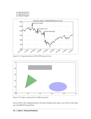
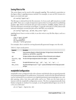
![The first argument to rc is the component you wish to customize, such as 'figure',
'axes', 'xtick', 'ytick', 'grid', 'legend' or many others. After that can follow a
sequence of keyword arguments indicating the new parameters. An easy way to write
down the options in your program is as a dict:
font_options = {'family' : 'monospace',
'weight' : 'bold',
'size' : 'small'}
plt.rc('font', **font_options)
For more extensive customization and to see a list of all the options, matplotlib comes
with a configuration file matplotlibrc in the matplotlib/mpl-data directory. If you cus-
tomize this file and place it in your home directory titled .matplotlibrc, it will be loaded
each time you use matplotlib.
Plotting Functions in pandas
As you’ve seen, matplotlib is actually a fairly low-level tool. You assemble a plot from
its base components: the data display (the type of plot: line, bar, box, scatter, contour,
etc.), legend, title, tick labels, and other annotations. Part of the reason for this is that
in many cases the data needed to make a complete plot is spread across many objects.
In pandas we have row labels, column labels, and possibly grouping information. This
means that many kinds of fully-formed plots that would ordinarily require a lot of
matplotlib code can be expressed in one or two concise statements. Therefore, pandas
has an increasing number of high-level plotting methods for creating standard visual-
izations that take advantage of how data is organized in DataFrame objects.
As of this writing, the plotting functionality in pandas is undergoing
quite a bit of work. As part of the 2012 Google Summer of Code pro-
gram, a student is working full time to add features and to make the
interface more consistent and usable. Thus, it’s possible that this code
may fall out-of-date faster than the other things in this book. The online
pandas documentation will be the best resource in that event.
Line Plots
Series and DataFrame each have a plot method for making many different plot types.
By default, they make line plots (see Figure 8-13):
In [55]: s = Series(np.random.randn(10).cumsum(), index=np.arange(0, 100, 10))
In [56]: s.plot()
The Series object’s index is passed to matplotlib for plotting on the X axis, though this
can be disabled by passing use_index=False. The X axis ticks and limits can be adjusted
using the xticks and xlim options, and Y axis respectively using yticks and ylim. See
232 | Chapter 8: Plotting and Visualization](https://image.slidesharecdn.com/wesmckinney-pythonfordataanalysis-oreillymedia2012-221114102054-a802e8f3/85/Wes-McKinney-Python-for-Data-Analysis-O-Reilly-Media-2012-pdf-248-320.jpg)
![Table 8-3 for a full listing of plot options. I’ll comment on a few more of them through-
out this section and leave the rest to you to explore.
Most of pandas’s plotting methods accept an optional ax parameter, which can be a
matplotlib subplot object. This gives you more flexible placement of subplots in a grid
layout. There will be more on this in the later section on the matplotlib API.
DataFrame’s plot method plots each of its columns as a different line on the same
subplot, creating a legend automatically (see Figure 8-14):
In [57]: df = DataFrame(np.random.randn(10, 4).cumsum(0),
....: columns=['A', 'B', 'C', 'D'],
....: index=np.arange(0, 100, 10))
In [58]: df.plot()
Additional keyword arguments to plot are passed through to the re-
spective matplotlib plotting function, so you can further customize
these plots by learning more about the matplotlib API.
Table 8-3. Series.plot method arguments
Argument Description
label Label for plot legend
ax matplotlib subplot object to plot on. If nothing passed, uses active matplotlib subplot
style Style string, like 'ko--', to be passed to matplotlib.
alpha The plot fill opacity (from 0 to 1)
Figure 8-13. Simple Series plot example
Plotting Functions in pandas | 233](https://image.slidesharecdn.com/wesmckinney-pythonfordataanalysis-oreillymedia2012-221114102054-a802e8f3/85/Wes-McKinney-Python-for-Data-Analysis-O-Reilly-Media-2012-pdf-249-320.jpg)
![Argument Description
kind Can be 'line', 'bar', 'barh', 'kde'
logy Use logarithmic scaling on the Y axis
use_index Use the object index for tick labels
rot Rotation of tick labels (0 through 360)
xticks Values to use for X axis ticks
yticks Values to use for Y axis ticks
xlim X axis limits (e.g. [0, 10])
ylim Y axis limits
grid Display axis grid (on by default)
DataFrame has a number of options allowing some flexibility with how the columns
are handled; for example, whether to plot them all on the same subplot or to create
separate subplots. See Table 8-4 for more on these.
Table 8-4. DataFrame-specific plot arguments
Argument Description
subplots Plot each DataFrame column in a separate subplot
sharex If subplots=True, share the same X axis, linking ticks and limits
sharey If subplots=True, share the same Y axis
figsize Size of figure to create as tuple
Figure 8-14. Simple DataFrame plot example
234 | Chapter 8: Plotting and Visualization](https://image.slidesharecdn.com/wesmckinney-pythonfordataanalysis-oreillymedia2012-221114102054-a802e8f3/85/Wes-McKinney-Python-for-Data-Analysis-O-Reilly-Media-2012-pdf-250-320.jpg)
![Argument Description
title Plot title as string
legend Add a subplot legend (True by default)
sort_columns Plot columns in alphabetical order; by default uses existing column order
For time series plotting, see Chapter 10.
Bar Plots
Making bar plots instead of line plots is a simple as passing kind='bar' (for vertical
bars) or kind='barh' (for horizontal bars). In this case, the Series or DataFrame index
will be used as the X (bar) or Y (barh) ticks (see Figure 8-15):
In [59]: fig, axes = plt.subplots(2, 1)
In [60]: data = Series(np.random.rand(16), index=list('abcdefghijklmnop'))
In [61]: data.plot(kind='bar', ax=axes[0], color='k', alpha=0.7)
Out[61]: <matplotlib.axes.AxesSubplot at 0x4ee7750>
In [62]: data.plot(kind='barh', ax=axes[1], color='k', alpha=0.7)
For more on the plt.subplots function and matplotlib axes and figures,
see the later section in this chapter.
With a DataFrame, bar plots group the values in each row together in a group in bars,
side by side, for each value. See Figure 8-16:
In [63]: df = DataFrame(np.random.rand(6, 4),
....: index=['one', 'two', 'three', 'four', 'five', 'six'],
....: columns=pd.Index(['A', 'B', 'C', 'D'], name='Genus'))
In [64]: df
Out[64]:
Genus A B C D
one 0.301686 0.156333 0.371943 0.270731
two 0.750589 0.525587 0.689429 0.358974
three 0.381504 0.667707 0.473772 0.632528
four 0.942408 0.180186 0.708284 0.641783
five 0.840278 0.909589 0.010041 0.653207
six 0.062854 0.589813 0.811318 0.060217
In [65]: df.plot(kind='bar')
Plotting Functions in pandas | 235](https://image.slidesharecdn.com/wesmckinney-pythonfordataanalysis-oreillymedia2012-221114102054-a802e8f3/85/Wes-McKinney-Python-for-Data-Analysis-O-Reilly-Media-2012-pdf-251-320.jpg)
![Figure 8-15. Horizonal and vertical bar plot example
Note that the name “Genus” on the DataFrame’s columns is used to title the legend.
Stacked bar plots are created from a DataFrame by passing stacked=True, resulting in
the value in each row being stacked together (see Figure 8-17):
In [67]: df.plot(kind='barh', stacked=True, alpha=0.5)
A useful recipe for bar plots (as seen in an earlier chapter) is to visualize
a Series’s value frequency using value_counts: s.value_counts
().plot(kind='bar')
Returning to the tipping data set used earlier in the book, suppose we wanted to make
a stacked bar plot showing the percentage of data points for each party size on each
day. I load the data using read_csv and make a cross-tabulation by day and party size:
In [68]: tips = pd.read_csv('ch08/tips.csv')
In [69]: party_counts = pd.crosstab(tips.day, tips.size)
In [70]: party_counts
Out[70]:
size 1 2 3 4 5 6
day
Fri 1 16 1 1 0 0
Sat 2 53 18 13 1 0
Sun 0 39 15 18 3 1
Thur 1 48 4 5 1 3
236 | Chapter 8: Plotting and Visualization](https://image.slidesharecdn.com/wesmckinney-pythonfordataanalysis-oreillymedia2012-221114102054-a802e8f3/85/Wes-McKinney-Python-for-Data-Analysis-O-Reilly-Media-2012-pdf-252-320.jpg)
![# Not many 1- and 6-person parties
In [71]: party_counts = party_counts.ix[:, 2:5]
Figure 8-16. DataFrame bar plot example
Figure 8-17. DataFrame stacked bar plot example
Then, normalize so that each row sums to 1 (I have to cast to float to avoid integer
division issues on Python 2.7) and make the plot (see Figure 8-18):
# Normalize to sum to 1
In [72]: party_pcts = party_counts.div(party_counts.sum(1).astype(float), axis=0)
Plotting Functions in pandas | 237](https://image.slidesharecdn.com/wesmckinney-pythonfordataanalysis-oreillymedia2012-221114102054-a802e8f3/85/Wes-McKinney-Python-for-Data-Analysis-O-Reilly-Media-2012-pdf-253-320.jpg)
![In [73]: party_pcts
Out[73]:
size 2 3 4 5
day
Fri 0.888889 0.055556 0.055556 0.000000
Sat 0.623529 0.211765 0.152941 0.011765
Sun 0.520000 0.200000 0.240000 0.040000
Thur 0.827586 0.068966 0.086207 0.017241
In [74]: party_pcts.plot(kind='bar', stacked=True)
Figure 8-18. Fraction of parties by size on each day
So you can see that party sizes appear to increase on the weekend in this data set.
Histograms and Density Plots
A histogram, with which you may be well-acquainted, is a kind of bar plot that gives a
discretized display of value frequency. The data points are split into discrete, evenly
spaced bins, and the number of data points in each bin is plotted. Using the tipping
data from before, we can make a histogram of tip percentages of the total bill using the
hist method on the Series (see Figure 8-19):
In [76]: tips['tip_pct'] = tips['tip'] / tips['total_bill']
In [77]: tips['tip_pct'].hist(bins=50)
238 | Chapter 8: Plotting and Visualization](https://image.slidesharecdn.com/wesmckinney-pythonfordataanalysis-oreillymedia2012-221114102054-a802e8f3/85/Wes-McKinney-Python-for-Data-Analysis-O-Reilly-Media-2012-pdf-254-320.jpg)
![Figure 8-19. Histogram of tip percentages
A related plot type is a density plot, which is formed by computing an estimate of a
continuous probability distribution that might have generated the observed data. A
usual procedure is to approximate this distribution as a mixture of kernels, that is,
simpler distributions like the normal (Gaussian) distribution. Thus, density plots are
also known as KDE (kernel density estimate) plots. Using plot with kind='kde' makes
a density plot using the standard mixture-of-normals KDE (see Figure 8-20):
In [79]: tips['tip_pct'].plot(kind='kde')
These two plot types are often plotted together; the histogram in normalized form (to
give a binned density) with a kernel density estimate plotted on top. As an example,
consider a bimodal distribution consisting of draws from two different standard normal
distributions (see Figure 8-21):
In [81]: comp1 = np.random.normal(0, 1, size=200) # N(0, 1)
In [82]: comp2 = np.random.normal(10, 2, size=200) # N(10, 4)
In [83]: values = Series(np.concatenate([comp1, comp2]))
In [84]: values.hist(bins=100, alpha=0.3, color='k', normed=True)
Out[84]: <matplotlib.axes.AxesSubplot at 0x5cd2350>
In [85]: values.plot(kind='kde', style='k--')
Scatter Plots
Scatter plots are a useful way of examining the relationship between two one-dimen-
sional data series. matplotlib has a scatter plotting method that is the workhorse of
Plotting Functions in pandas | 239](https://image.slidesharecdn.com/wesmckinney-pythonfordataanalysis-oreillymedia2012-221114102054-a802e8f3/85/Wes-McKinney-Python-for-Data-Analysis-O-Reilly-Media-2012-pdf-255-320.jpg)
![making these kinds of plots. To give an example, I load the macrodata dataset from the
statsmodels project, select a few variables, then compute log differences:
In [86]: macro = pd.read_csv('ch08/macrodata.csv')
In [87]: data = macro[['cpi', 'm1', 'tbilrate', 'unemp']]
In [88]: trans_data = np.log(data).diff().dropna()
Figure 8-20. Density plot of tip percentages
Figure 8-21. Normalized histogram of normal mixture with density estimate
240 | Chapter 8: Plotting and Visualization](https://image.slidesharecdn.com/wesmckinney-pythonfordataanalysis-oreillymedia2012-221114102054-a802e8f3/85/Wes-McKinney-Python-for-Data-Analysis-O-Reilly-Media-2012-pdf-256-320.jpg)
![In [89]: trans_data[-5:]
Out[89]:
cpi m1 tbilrate unemp
198 -0.007904 0.045361 -0.396881 0.105361
199 -0.021979 0.066753 -2.277267 0.139762
200 0.002340 0.010286 0.606136 0.160343
201 0.008419 0.037461 -0.200671 0.127339
202 0.008894 0.012202 -0.405465 0.042560
It’s easy to plot a simple scatter plot using plt.scatter (see Figure 8-22):
In [91]: plt.scatter(trans_data['m1'], trans_data['unemp'])
Out[91]: <matplotlib.collections.PathCollection at 0x43c31d0>
In [92]: plt.title('Changes in log %s vs. log %s' % ('m1', 'unemp'))
Figure 8-22. A simple scatter plot
In exploratory data analysis it’s helpful to be able to look at all the scatter plots among
a group of variables; this is known as a pairs plot or scatter plot matrix. Making such a
plot from scratch is a bit of work, so pandas has a scatter_matrix function for creating
one from a DataFrame. It also supports placing histograms or density plots of each
variable along the diagonal. See Figure 8-23 for the resulting plot:
In [93]: scatter_matrix(trans_data, diagonal='kde', color='k', alpha=0.3)
Plotting Maps: Visualizing Haiti Earthquake Crisis Data
Ushahidi is a non-profit software company that enables crowdsourcing of information
related to natural disasters and geopolitical events via text message. Many of these data
sets are then published on their website for analysis and visualization. I downloaded
Plotting Maps: Visualizing Haiti Earthquake Crisis Data | 241](https://image.slidesharecdn.com/wesmckinney-pythonfordataanalysis-oreillymedia2012-221114102054-a802e8f3/85/Wes-McKinney-Python-for-Data-Analysis-O-Reilly-Media-2012-pdf-257-320.jpg)
![the data collected during the 2010 Haiti earthquake crisis and aftermath, and I’ll show
you how I prepared the data for analysis and visualization using pandas and other tools
we have looked at thus far. After downloading the CSV file from the above link, we can
load it into a DataFrame using read_csv:
In [94]: data = pd.read_csv('ch08/Haiti.csv')
In [95]: data
Out[95]:
<class 'pandas.core.frame.DataFrame'>
Int64Index: 3593 entries, 0 to 3592
Data columns:
Serial 3593 non-null values
INCIDENT TITLE 3593 non-null values
INCIDENT DATE 3593 non-null values
LOCATION 3593 non-null values
DESCRIPTION 3593 non-null values
CATEGORY 3587 non-null values
LATITUDE 3593 non-null values
LONGITUDE 3593 non-null values
APPROVED 3593 non-null values
VERIFIED 3593 non-null values
dtypes: float64(2), int64(1), object(7)
It’s easy now to tinker with this data set to see what kinds of things we might want to
do with it. Each row represents a report sent from someone’s mobile phone indicating
an emergency or some other problem. Each has an associated timestamp and a location
as latitude and longitude:
In [96]: data[['INCIDENT DATE', 'LATITUDE', 'LONGITUDE']][:10]
Out[96]:
INCIDENT DATE LATITUDE LONGITUDE
Figure 8-23. Scatter plot matrix of statsmodels macro data
242 | Chapter 8: Plotting and Visualization](https://image.slidesharecdn.com/wesmckinney-pythonfordataanalysis-oreillymedia2012-221114102054-a802e8f3/85/Wes-McKinney-Python-for-Data-Analysis-O-Reilly-Media-2012-pdf-258-320.jpg)
![0 05/07/2010 17:26 18.233333 -72.533333
1 28/06/2010 23:06 50.226029 5.729886
2 24/06/2010 16:21 22.278381 114.174287
3 20/06/2010 21:59 44.407062 8.933989
4 18/05/2010 16:26 18.571084 -72.334671
5 26/04/2010 13:14 18.593707 -72.310079
6 26/04/2010 14:19 18.482800 -73.638800
7 26/04/2010 14:27 18.415000 -73.195000
8 15/03/2010 10:58 18.517443 -72.236841
9 15/03/2010 11:00 18.547790 -72.410010
The CATEGORY field contains a comma-separated list of codes indicating the type of
message:
In [97]: data['CATEGORY'][:6]
Out[97]:
0 1. Urgences | Emergency, 3. Public Health,
1 1. Urgences | Emergency, 2. Urgences logistiques
2 2. Urgences logistiques | Vital Lines, 8. Autre |
3 1. Urgences | Emergency,
4 1. Urgences | Emergency,
5 5e. Communication lines down,
Name: CATEGORY
If you notice above in the data summary, some of the categories are missing, so we
might want to drop these data points. Additionally, calling describe shows that there
are some aberrant locations:
In [98]: data.describe()
Out[98]:
Serial LATITUDE LONGITUDE
count 3593.000000 3593.000000 3593.000000
mean 2080.277484 18.611495 -72.322680
std 1171.100360 0.738572 3.650776
min 4.000000 18.041313 -74.452757
25% 1074.000000 18.524070 -72.417500
50% 2163.000000 18.539269 -72.335000
75% 3088.000000 18.561820 -72.293570
max 4052.000000 50.226029 114.174287
Cleaning the bad locations and removing the missing categories is now fairly simple:
In [99]: data = data[(data.LATITUDE > 18) & (data.LATITUDE < 20) &
....: (data.LONGITUDE > -75) & (data.LONGITUDE < -70)
....: & data.CATEGORY.notnull()]
Now we might want to do some analysis or visualization of this data by category, but
each category field may have multiple categories. Additionally, each category is given
as a code plus an English and possibly also a French code name. Thus, a little bit of
wrangling is required to get the data into a more agreeable form. First, I wrote these
two functions to get a list of all the categories and to split each category into a code and
an English name:
def to_cat_list(catstr):
stripped = (x.strip() for x in catstr.split(','))
Plotting Maps: Visualizing Haiti Earthquake Crisis Data | 243](https://image.slidesharecdn.com/wesmckinney-pythonfordataanalysis-oreillymedia2012-221114102054-a802e8f3/85/Wes-McKinney-Python-for-Data-Analysis-O-Reilly-Media-2012-pdf-259-320.jpg)
![return [x for x in stripped if x]
def get_all_categories(cat_series):
cat_sets = (set(to_cat_list(x)) for x in cat_series)
return sorted(set.union(*cat_sets))
def get_english(cat):
code, names = cat.split('.')
if '|' in names:
names = names.split(' | ')[1]
return code, names.strip()
You can test out that the get_english function does what you expect:
In [101]: get_english('2. Urgences logistiques | Vital Lines')
Out[101]: ('2', 'Vital Lines')
Now, I make a dict mapping code to name because we’ll use the codes for analysis.
We’ll use this later when adorning plots (note the use of a generator expression in lieu
of a list comprehension):
In [102]: all_cats = get_all_categories(data.CATEGORY)
# Generator expression
In [103]: english_mapping = dict(get_english(x) for x in all_cats)
In [104]: english_mapping['2a']
Out[104]: 'Food Shortage'
In [105]: english_mapping['6c']
Out[105]: 'Earthquake and aftershocks'
There are many ways to go about augmenting the data set to be able to easily select
records by category. One way is to add indicator (or dummy) columns, one for each
category. To do that, first extract the unique category codes and construct a DataFrame
of zeros having those as its columns and the same index as data:
def get_code(seq):
return [x.split('.')[0] for x in seq if x]
all_codes = get_code(all_cats)
code_index = pd.Index(np.unique(all_codes))
dummy_frame = DataFrame(np.zeros((len(data), len(code_index))),
index=data.index, columns=code_index)
If all goes well, dummy_frame should look something like this:
In [107]: dummy_frame.ix[:, :6]
Out[107]:
<class 'pandas.core.frame.DataFrame'>
Int64Index: 3569 entries, 0 to 3592
Data columns:
1 3569 non-null values
1a 3569 non-null values
1b 3569 non-null values
1c 3569 non-null values
244 | Chapter 8: Plotting and Visualization](https://image.slidesharecdn.com/wesmckinney-pythonfordataanalysis-oreillymedia2012-221114102054-a802e8f3/85/Wes-McKinney-Python-for-Data-Analysis-O-Reilly-Media-2012-pdf-260-320.jpg)
![1d 3569 non-null values
2 3569 non-null values
dtypes: float64(6)
As you recall, the trick is then to set the appropriate entries of each row to 1, lastly
joining this with data:
for row, cat in zip(data.index, data.CATEGORY):
codes = get_code(to_cat_list(cat))
dummy_frame.ix[row, codes] = 1
data = data.join(dummy_frame.add_prefix('category_'))
data finally now has new columns like:
In [109]: data.ix[:, 10:15]
Out[109]:
<class 'pandas.core.frame.DataFrame'>
Int64Index: 3569 entries, 0 to 3592
Data columns:
category_1 3569 non-null values
category_1a 3569 non-null values
category_1b 3569 non-null values
category_1c 3569 non-null values
category_1d 3569 non-null values
dtypes: float64(5)
Let’s make some plots! As this is spatial data, we’d like to plot the data by category on
a map of Haiti. The basemap toolkit (http://matplotlib.github.com/basemap), an add-on
to matplotlib, enables plotting 2D data on maps in Python. basemap provides many
different globe projections and a means for transforming projecting latitude and lon-
gitude coordinates on the globe onto a two-dimensional matplotlib plot. After some
trial and error and using the above data as a guideline, I wrote this function which draws
a simple black and white map of Haiti:
from mpl_toolkits.basemap import Basemap
import matplotlib.pyplot as plt
def basic_haiti_map(ax=None, lllat=17.25, urlat=20.25,
lllon=-75, urlon=-71):
# create polar stereographic Basemap instance.
m = Basemap(ax=ax, projection='stere',
lon_0=(urlon + lllon) / 2,
lat_0=(urlat + lllat) / 2,
llcrnrlat=lllat, urcrnrlat=urlat,
llcrnrlon=lllon, urcrnrlon=urlon,
resolution='f')
# draw coastlines, state and country boundaries, edge of map.
m.drawcoastlines()
m.drawstates()
m.drawcountries()
return m
The idea, now, is that the returned Basemap object, knows how to transform coordinates
onto the canvas. I wrote the following code to plot the data observations for a number
Plotting Maps: Visualizing Haiti Earthquake Crisis Data | 245](https://image.slidesharecdn.com/wesmckinney-pythonfordataanalysis-oreillymedia2012-221114102054-a802e8f3/85/Wes-McKinney-Python-for-Data-Analysis-O-Reilly-Media-2012-pdf-261-320.jpg)
![of report categories. For each category, I filter down the data set to the coordinates
labeled by that category, plot a Basemap on the appropriate subplot, transform the co-
ordinates, then plot the points using the Basemap’s plot method:
fig, axes = plt.subplots(nrows=2, ncols=2, figsize=(12, 10))
fig.subplots_adjust(hspace=0.05, wspace=0.05)
to_plot = ['2a', '1', '3c', '7a']
lllat=17.25; urlat=20.25; lllon=-75; urlon=-71
for code, ax in zip(to_plot, axes.flat):
m = basic_haiti_map(ax, lllat=lllat, urlat=urlat,
lllon=lllon, urlon=urlon)
cat_data = data[data['category_%s' % code] == 1]
# compute map proj coordinates.
x, y = m(cat_data.LONGITUDE, cat_data.LATITUDE)
m.plot(x, y, 'k.', alpha=0.5)
ax.set_title('%s: %s' % (code, english_mapping[code]))
The resulting figure can be seen in Figure 8-24.
It seems from the plot that most of the data is concentrated around the most populous
city, Port-au-Prince. basemap allows you to overlap additional map data which comes
from what are called shapefiles. I first downloaded a shapefile with roads in Port-au-
Prince (see http://cegrp.cga.harvard.edu/haiti/?q=resources_data). The Basemap object
conveniently has a readshapefile method so that, after extracting the road data archive,
I added just the following lines to my code:
Figure 8-24. Haiti crisis data for 4 categories
246 | Chapter 8: Plotting and Visualization](https://image.slidesharecdn.com/wesmckinney-pythonfordataanalysis-oreillymedia2012-221114102054-a802e8f3/85/Wes-McKinney-Python-for-Data-Analysis-O-Reilly-Media-2012-pdf-262-320.jpg)
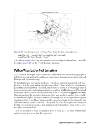
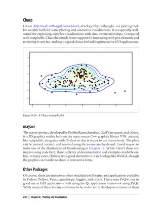


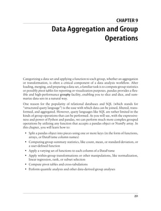
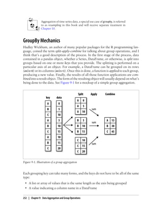
![• A dict or Series giving a correspondence between the values on the axis being
grouped and the group names
• A function to be invoked on the axis index or the individual labels in the index
Note that the latter three methods are all just shortcuts for producing an array of values
to be used to split up the object. Don’t worry if this all seems very abstract. Throughout
this chapter, I will give many examples of all of these methods. To get started, here is
a very simple small tabular dataset as a DataFrame:
In [13]: df = DataFrame({'key1' : ['a', 'a', 'b', 'b', 'a'],
....: 'key2' : ['one', 'two', 'one', 'two', 'one'],
....: 'data1' : np.random.randn(5),
....: 'data2' : np.random.randn(5)})
In [14]: df
Out[14]:
data1 data2 key1 key2
0 -0.204708 1.393406 a one
1 0.478943 0.092908 a two
2 -0.519439 0.281746 b one
3 -0.555730 0.769023 b two
4 1.965781 1.246435 a one
Suppose you wanted to compute the mean of the data1 column using the groups labels
from key1. There are a number of ways to do this. One is to access data1 and call
groupby with the column (a Series) at key1:
In [15]: grouped = df['data1'].groupby(df['key1'])
In [16]: grouped
Out[16]: <pandas.core.groupby.SeriesGroupBy at 0x2d78b10>
This grouped variable is now a GroupBy object. It has not actually computed anything
yet except for some intermediate data about the group key df['key1']. The idea is that
this object has all of the information needed to then apply some operation to each of
the groups. For example, to compute group means we can call the GroupBy’s mean
method:
In [17]: grouped.mean()
Out[17]:
key1
a 0.746672
b -0.537585
Later, I'll explain more about what’s going on when you call .mean(). The important
thing here is that the data (a Series) has been aggregated according to the group key,
producing a new Series that is now indexed by the unique values in the key1 column.
The result index has the name 'key1' because the DataFrame column df['key1'] did.
If instead we had passed multiple arrays as a list, we get something different:
In [18]: means = df['data1'].groupby([df['key1'], df['key2']]).mean()
GroupBy Mechanics | 253](https://image.slidesharecdn.com/wesmckinney-pythonfordataanalysis-oreillymedia2012-221114102054-a802e8f3/85/Wes-McKinney-Python-for-Data-Analysis-O-Reilly-Media-2012-pdf-269-320.jpg)
![In [19]: means
Out[19]:
key1 key2
a one 0.880536
two 0.478943
b one -0.519439
two -0.555730
In this case, we grouped the data using two keys, and the resulting Series now has a
hierarchical index consisting of the unique pairs of keys observed:
In [20]: means.unstack()
Out[20]:
key2 one two
key1
a 0.880536 0.478943
b -0.519439 -0.555730
In these examples, the group keys are all Series, though they could be any arrays of the
right length:
In [21]: states = np.array(['Ohio', 'California', 'California', 'Ohio', 'Ohio'])
In [22]: years = np.array([2005, 2005, 2006, 2005, 2006])
In [23]: df['data1'].groupby([states, years]).mean()
Out[23]:
California 2005 0.478943
2006 -0.519439
Ohio 2005 -0.380219
2006 1.965781
Frequently the grouping information to be found in the same DataFrame as the data
you want to work on. In that case, you can pass column names (whether those are
strings, numbers, or other Python objects) as the group keys:
In [24]: df.groupby('key1').mean()
Out[24]:
data1 data2
key1
a 0.746672 0.910916
b -0.537585 0.525384
In [25]: df.groupby(['key1', 'key2']).mean()
Out[25]:
data1 data2
key1 key2
a one 0.880536 1.319920
two 0.478943 0.092908
b one -0.519439 0.281746
two -0.555730 0.769023
You may have noticed in the first case df.groupby('key1').mean() that there is no
key2 column in the result. Because df['key2'] is not numeric data, it is said to be a
nuisance column, which is therefore excluded from the result. By default, all of the
254 | Chapter 9: Data Aggregation and Group Operations](https://image.slidesharecdn.com/wesmckinney-pythonfordataanalysis-oreillymedia2012-221114102054-a802e8f3/85/Wes-McKinney-Python-for-Data-Analysis-O-Reilly-Media-2012-pdf-270-320.jpg)
![numeric columns are aggregated, though it is possible to filter down to a subset as you’ll
see soon.
Regardless of the objective in using groupby, a generally useful GroupBy method is
size which return a Series containing group sizes:
In [26]: df.groupby(['key1', 'key2']).size()
Out[26]:
key1 key2
a one 2
two 1
b one 1
two 1
As of this writing, any missing values in a group key will be excluded
from the result. It’s possible (and, in fact, quite likely), that by the time
you are reading this there will be an option to include the NA group in
the result.
Iterating Over Groups
The GroupBy object supports iteration, generating a sequence of 2-tuples containing
the group name along with the chunk of data. Consider the following small example
data set:
In [27]: for name, group in df.groupby('key1'):
....: print name
....: print group
....:
a
data1 data2 key1 key2
0 -0.204708 1.393406 a one
1 0.478943 0.092908 a two
4 1.965781 1.246435 a one
b
data1 data2 key1 key2
2 -0.519439 0.281746 b one
3 -0.555730 0.769023 b two
In the case of multiple keys, the first element in the tuple will be a tuple of key values:
In [28]: for (k1, k2), group in df.groupby(['key1', 'key2']):
....: print k1, k2
....: print group
....:
a one
data1 data2 key1 key2
0 -0.204708 1.393406 a one
4 1.965781 1.246435 a one
a two
data1 data2 key1 key2
1 0.478943 0.092908 a two
b one
data1 data2 key1 key2
GroupBy Mechanics | 255](https://image.slidesharecdn.com/wesmckinney-pythonfordataanalysis-oreillymedia2012-221114102054-a802e8f3/85/Wes-McKinney-Python-for-Data-Analysis-O-Reilly-Media-2012-pdf-271-320.jpg)
![2 -0.519439 0.281746 b one
b two
data1 data2 key1 key2
3 -0.55573 0.769023 b two
Of course, you can choose to do whatever you want with the pieces of data. A recipe
you may find useful is computing a dict of the data pieces as a one-liner:
In [29]: pieces = dict(list(df.groupby('key1')))
In [30]: pieces['b']
Out[30]:
data1 data2 key1 key2
2 -0.519439 0.281746 b one
3 -0.555730 0.769023 b two
By default groupby groups on axis=0, but you can group on any of the other axes. For
example, we could group the columns of our example df here by dtype like so:
In [31]: df.dtypes
Out[31]:
data1 float64
data2 float64
key1 object
key2 object
In [32]: grouped = df.groupby(df.dtypes, axis=1)
In [33]: dict(list(grouped))
Out[33]:
{dtype('float64'): data1 data2
0 -0.204708 1.393406
1 0.478943 0.092908
2 -0.519439 0.281746
3 -0.555730 0.769023
4 1.965781 1.246435,
dtype('object'): key1 key2
0 a one
1 a two
2 b one
3 b two
4 a one}
Selecting a Column or Subset of Columns
Indexing a GroupBy object created from a DataFrame with a column name or array of
column names has the effect of selecting those columns for aggregation. This means that:
df.groupby('key1')['data1']
df.groupby('key1')[['data2']]
are syntactic sugar for:
df['data1'].groupby(df['key1'])
df[['data2']].groupby(df['key1'])
256 | Chapter 9: Data Aggregation and Group Operations](https://image.slidesharecdn.com/wesmckinney-pythonfordataanalysis-oreillymedia2012-221114102054-a802e8f3/85/Wes-McKinney-Python-for-Data-Analysis-O-Reilly-Media-2012-pdf-272-320.jpg)
![Especially for large data sets, it may be desirable to aggregate only a few columns. For
example, in the above data set, to compute means for just the data2 column and get
the result as a DataFrame, we could write:
In [34]: df.groupby(['key1', 'key2'])[['data2']].mean()
Out[34]:
data2
key1 key2
a one 1.319920
two 0.092908
b one 0.281746
two 0.769023
The object returned by this indexing operation is a grouped DataFrame if a list or array
is passed and a grouped Series is just a single column name that is passed as a scalar:
In [35]: s_grouped = df.groupby(['key1', 'key2'])['data2']
In [36]: s_grouped
Out[36]: <pandas.core.groupby.SeriesGroupBy at 0x2e215d0>
In [37]: s_grouped.mean()
Out[37]:
key1 key2
a one 1.319920
two 0.092908
b one 0.281746
two 0.769023
Name: data2
Grouping with Dicts and Series
Grouping information may exist in a form other than an array. Let’s consider another
example DataFrame:
In [38]: people = DataFrame(np.random.randn(5, 5),
....: columns=['a', 'b', 'c', 'd', 'e'],
....: index=['Joe', 'Steve', 'Wes', 'Jim', 'Travis'])
In [39]: people.ix[2:3, ['b', 'c']] = np.nan # Add a few NA values
In [40]: people
Out[40]:
a b c d e
Joe 1.007189 -1.296221 0.274992 0.228913 1.352917
Steve 0.886429 -2.001637 -0.371843 1.669025 -0.438570
Wes -0.539741 NaN NaN -1.021228 -0.577087
Jim 0.124121 0.302614 0.523772 0.000940 1.343810
Travis -0.713544 -0.831154 -2.370232 -1.860761 -0.860757
Now, suppose I have a group correspondence for the columns and want to sum together
the columns by group:
In [41]: mapping = {'a': 'red', 'b': 'red', 'c': 'blue',
....: 'd': 'blue', 'e': 'red', 'f' : 'orange'}
GroupBy Mechanics | 257](https://image.slidesharecdn.com/wesmckinney-pythonfordataanalysis-oreillymedia2012-221114102054-a802e8f3/85/Wes-McKinney-Python-for-Data-Analysis-O-Reilly-Media-2012-pdf-273-320.jpg)
![Now, you could easily construct an array from this dict to pass to groupby, but instead
we can just pass the dict:
In [42]: by_column = people.groupby(mapping, axis=1)
In [43]: by_column.sum()
Out[43]:
blue red
Joe 0.503905 1.063885
Steve 1.297183 -1.553778
Wes -1.021228 -1.116829
Jim 0.524712 1.770545
Travis -4.230992 -2.405455
The same functionality holds for Series, which can be viewed as a fixed size mapping.
When I used Series as group keys in the above examples, pandas does, in fact, inspect
each Series to ensure that its index is aligned with the axis it’s grouping:
In [44]: map_series = Series(mapping)
In [45]: map_series
Out[45]:
a red
b red
c blue
d blue
e red
f orange
In [46]: people.groupby(map_series, axis=1).count()
Out[46]:
blue red
Joe 2 3
Steve 2 3
Wes 1 2
Jim 2 3
Travis 2 3
Grouping with Functions
Using Python functions in what can be fairly creative ways is a more abstract way of
defining a group mapping compared with a dict or Series. Any function passed as a
group key will be called once per index value, with the return values being used as the
group names. More concretely, consider the example DataFrame from the previous
section, which has people’s first names as index values. Suppose you wanted to group
by the length of the names; you could compute an array of string lengths, but instead
you can just pass the len function:
In [47]: people.groupby(len).sum()
Out[47]:
a b c d e
3 0.591569 -0.993608 0.798764 -0.791374 2.119639
258 | Chapter 9: Data Aggregation and Group Operations](https://image.slidesharecdn.com/wesmckinney-pythonfordataanalysis-oreillymedia2012-221114102054-a802e8f3/85/Wes-McKinney-Python-for-Data-Analysis-O-Reilly-Media-2012-pdf-274-320.jpg)
![5 0.886429 -2.001637 -0.371843 1.669025 -0.438570
6 -0.713544 -0.831154 -2.370232 -1.860761 -0.860757
Mixing functions with arrays, dicts, or Series is not a problem as everything gets con-
verted to arrays internally:
In [48]: key_list = ['one', 'one', 'one', 'two', 'two']
In [49]: people.groupby([len, key_list]).min()
Out[49]:
a b c d e
3 one -0.539741 -1.296221 0.274992 -1.021228 -0.577087
two 0.124121 0.302614 0.523772 0.000940 1.343810
5 one 0.886429 -2.001637 -0.371843 1.669025 -0.438570
6 two -0.713544 -0.831154 -2.370232 -1.860761 -0.860757
Grouping by Index Levels
A final convenience for hierarchically-indexed data sets is the ability to aggregate using
one of the levels of an axis index. To do this, pass the level number or name using the
level keyword:
In [50]: columns = pd.MultiIndex.from_arrays([['US', 'US', 'US', 'JP', 'JP'],
....: [1, 3, 5, 1, 3]], names=['cty', 'tenor'])
In [51]: hier_df = DataFrame(np.random.randn(4, 5), columns=columns)
In [52]: hier_df
Out[52]:
cty US JP
tenor 1 3 5 1 3
0 0.560145 -1.265934 0.119827 -1.063512 0.332883
1 -2.359419 -0.199543 -1.541996 -0.970736 -1.307030
2 0.286350 0.377984 -0.753887 0.331286 1.349742
3 0.069877 0.246674 -0.011862 1.004812 1.327195
In [53]: hier_df.groupby(level='cty', axis=1).count()
Out[53]:
cty JP US
0 2 3
1 2 3
2 2 3
3 2 3
Data Aggregation
By aggregation, I am generally referring to any data transformation that produces scalar
values from arrays. In the examples above I have used several of them, such as mean,
count, min and sum. You may wonder what is going on when you invoke mean() on a
GroupBy object. Many common aggregations, such as those found in Table 9-1, have
optimized implementations that compute the statistics on the dataset in place. How-
ever, you are not limited to only this set of methods. You can use aggregations of your
Data Aggregation | 259](https://image.slidesharecdn.com/wesmckinney-pythonfordataanalysis-oreillymedia2012-221114102054-a802e8f3/85/Wes-McKinney-Python-for-Data-Analysis-O-Reilly-Media-2012-pdf-275-320.jpg)
![own devising and additionally call any method that is also defined on the grouped
object. For example, as you recall quantile computes sample quantiles of a Series or a
DataFrame’s columns 1:
In [54]: df
Out[54]:
data1 data2 key1 key2
0 -0.204708 1.393406 a one
1 0.478943 0.092908 a two
2 -0.519439 0.281746 b one
3 -0.555730 0.769023 b two
4 1.965781 1.246435 a one
In [55]: grouped = df.groupby('key1')
In [56]: grouped['data1'].quantile(0.9)
Out[56]:
key1
a 1.668413
b -0.523068
While quantile is not explicitly implemented for GroupBy, it is a Series method and
thus available for use. Internally, GroupBy efficiently slices up the Series, calls
piece.quantile(0.9) foreachpiece,thenassemblesthoseresultstogetherintotheresult
object.
To use your own aggregation functions, pass any function that aggregates an array to
the aggregate or agg method:
In [57]: def peak_to_peak(arr):
....: return arr.max() - arr.min()
In [58]: grouped.agg(peak_to_peak)
Out[58]:
data1 data2
key1
a 2.170488 1.300498
b 0.036292 0.487276
You’ll notice that some methods like describe also work, even though they are not
aggregations, strictly speaking:
In [59]: grouped.describe()
Out[59]:
data1 data2
key1
a count 3.000000 3.000000
mean 0.746672 0.910916
std 1.109736 0.712217
min -0.204708 0.092908
25% 0.137118 0.669671
50% 0.478943 1.246435
1. Note that quantile performs linear interpolation if there is no value at exactly the passed percentile.
260 | Chapter 9: Data Aggregation and Group Operations](https://image.slidesharecdn.com/wesmckinney-pythonfordataanalysis-oreillymedia2012-221114102054-a802e8f3/85/Wes-McKinney-Python-for-Data-Analysis-O-Reilly-Media-2012-pdf-276-320.jpg)
![75% 1.222362 1.319920
max 1.965781 1.393406
b count 2.000000 2.000000
mean -0.537585 0.525384
std 0.025662 0.344556
min -0.555730 0.281746
25% -0.546657 0.403565
50% -0.537585 0.525384
75% -0.528512 0.647203
max -0.519439 0.769023
I will explain in more detail what has happened here in the next major section on group-
wise operations and transformations.
Youmaynoticethatcustomaggregationfunctionsaremuchslowerthan
the optimized functions found in Table 9-1. This is because there is
significant overhead (function calls, data rearrangement) in construct-
ing the intermediate group data chunks.
Table 9-1. Optimized groupby methods
Function name Description
count Number of non-NA values in the group
sum Sum of non-NA values
mean Mean of non-NA values
median Arithmetic median of non-NA values
std, var Unbiased (n - 1 denominator) standard deviation and variance
min, max Minimum and maximum of non-NA values
prod Product of non-NA values
first, last First and last non-NA values
To illustrate some more advanced aggregation features, I’ll use a less trivial dataset, a
dataset on restaurant tipping. I obtained it from the R reshape2 package; it was origi-
nallyfoundinBryant&Smith’s1995textonbusinessstatistics(andfoundinthebook’s
GitHub repository). After loading it with read_csv, I add a tipping percentage column
tip_pct.
In [60]: tips = pd.read_csv('ch08/tips.csv')
# Add tip percentage of total bill
In [61]: tips['tip_pct'] = tips['tip'] / tips['total_bill']
In [62]: tips[:6]
Out[62]:
total_bill tip sex smoker day time size tip_pct
0 16.99 1.01 Female No Sun Dinner 2 0.059447
1 10.34 1.66 Male No Sun Dinner 3 0.160542
Data Aggregation | 261](https://image.slidesharecdn.com/wesmckinney-pythonfordataanalysis-oreillymedia2012-221114102054-a802e8f3/85/Wes-McKinney-Python-for-Data-Analysis-O-Reilly-Media-2012-pdf-277-320.jpg)
![2 21.01 3.50 Male No Sun Dinner 3 0.166587
3 23.68 3.31 Male No Sun Dinner 2 0.139780
4 24.59 3.61 Female No Sun Dinner 4 0.146808
5 25.29 4.71 Male No Sun Dinner 4 0.186240
Column-wise and Multiple Function Application
As you’ve seen above, aggregating a Series or all of the columns of a DataFrame is a
matter of using aggregate with the desired function or calling a method like mean or
std. However, you may want to aggregate using a different function depending on the
column or multiple functions at once. Fortunately, this is straightforward to do, which
I’ll illustrate through a number of examples. First, I’ll group the tips by sex and smoker:
In [63]: grouped = tips.groupby(['sex', 'smoker'])
Note that for descriptive statistics like those in Table 9-1, you can pass the name of the
function as a string:
In [64]: grouped_pct = grouped['tip_pct']
In [65]: grouped_pct.agg('mean')
Out[65]:
sex smoker
Female No 0.156921
Yes 0.182150
Male No 0.160669
Yes 0.152771
Name: tip_pct
If you pass a list of functions or function names instead, you get back a DataFrame with
column names taken from the functions:
In [66]: grouped_pct.agg(['mean', 'std', peak_to_peak])
Out[66]:
mean std peak_to_peak
sex smoker
Female No 0.156921 0.036421 0.195876
Yes 0.182150 0.071595 0.360233
Male No 0.160669 0.041849 0.220186
Yes 0.152771 0.090588 0.674707
You don’t need to accept the names that GroupBy gives to the columns; notably
lambda functions have the name '<lambda>' which make them hard to identify (you can
see for yourself by looking at a function’s __name__ attribute). As such, if you pass a list
of (name, function) tuples, the first element of each tuple will be used as the DataFrame
column names (you can think of a list of 2-tuples as an ordered mapping):
In [67]: grouped_pct.agg([('foo', 'mean'), ('bar', np.std)])
Out[67]:
foo bar
sex smoker
Female No 0.156921 0.036421
Yes 0.182150 0.071595
262 | Chapter 9: Data Aggregation and Group Operations](https://image.slidesharecdn.com/wesmckinney-pythonfordataanalysis-oreillymedia2012-221114102054-a802e8f3/85/Wes-McKinney-Python-for-Data-Analysis-O-Reilly-Media-2012-pdf-278-320.jpg)
![Male No 0.160669 0.041849
Yes 0.152771 0.090588
With a DataFrame, you have more options as you can specify a list of functions to apply
to all of the columns or different functions per column. To start, suppose we wanted
to compute the same three statistics for the tip_pct and total_bill columns:
In [68]: functions = ['count', 'mean', 'max']
In [69]: result = grouped['tip_pct', 'total_bill'].agg(functions)
In [70]: result
Out[70]:
tip_pct total_bill
count mean max count mean max
sex smoker
Female No 54 0.156921 0.252672 54 18.105185 35.83
Yes 33 0.182150 0.416667 33 17.977879 44.30
Male No 97 0.160669 0.291990 97 19.791237 48.33
Yes 60 0.152771 0.710345 60 22.284500 50.81
As you can see, the resulting DataFrame has hierarchical columns, the same as you
would get aggregating each column separately and using concat to glue the results
together using the column names as the keys argument:
In [71]: result['tip_pct']
Out[71]:
count mean max
sex smoker
Female No 54 0.156921 0.252672
Yes 33 0.182150 0.416667
Male No 97 0.160669 0.291990
Yes 60 0.152771 0.710345
As above, a list of tuples with custom names can be passed:
In [72]: ftuples = [('Durchschnitt', 'mean'), ('Abweichung', np.var)]
In [73]: grouped['tip_pct', 'total_bill'].agg(ftuples)
Out[73]:
tip_pct total_bill
Durchschnitt Abweichung Durchschnitt Abweichung
sex smoker
Female No 0.156921 0.001327 18.105185 53.092422
Yes 0.182150 0.005126 17.977879 84.451517
Male No 0.160669 0.001751 19.791237 76.152961
Yes 0.152771 0.008206 22.284500 98.244673
Now, suppose you wanted to apply potentially different functions to one or more of
the columns. The trick is to pass a dict to agg that contains a mapping of column names
to any of the function specifications listed so far:
In [74]: grouped.agg({'tip' : np.max, 'size' : 'sum'})
Out[74]:
size tip
sex smoker
Data Aggregation | 263](https://image.slidesharecdn.com/wesmckinney-pythonfordataanalysis-oreillymedia2012-221114102054-a802e8f3/85/Wes-McKinney-Python-for-Data-Analysis-O-Reilly-Media-2012-pdf-279-320.jpg)
![Female No 140 5.2
Yes 74 6.5
Male No 263 9.0
Yes 150 10.0
In [75]: grouped.agg({'tip_pct' : ['min', 'max', 'mean', 'std'],
....: 'size' : 'sum'})
Out[75]:
tip_pct size
min max mean std sum
sex smoker
Female No 0.056797 0.252672 0.156921 0.036421 140
Yes 0.056433 0.416667 0.182150 0.071595 74
Male No 0.071804 0.291990 0.160669 0.041849 263
Yes 0.035638 0.710345 0.152771 0.090588 150
A DataFrame will have hierarchical columns only if multiple functions are applied to
at least one column.
Returning Aggregated Data in “unindexed” Form
In all of the examples up until now, the aggregated data comes back with an index,
potentially hierarchical, composed from the unique group key combinations observed.
Since this isn’t always desirable, you can disable this behavior in most cases by passing
as_index=False to groupby:
In [76]: tips.groupby(['sex', 'smoker'], as_index=False).mean()
Out[76]:
sex smoker total_bill tip size tip_pct
0 Female No 18.105185 2.773519 2.592593 0.156921
1 Female Yes 17.977879 2.931515 2.242424 0.182150
2 Male No 19.791237 3.113402 2.711340 0.160669
3 Male Yes 22.284500 3.051167 2.500000 0.152771
Of course, it’s always possible to obtain the result in this format by calling
reset_index on the result.
Using groupby in this way is generally less flexible; results with hier-
archical columns, for example, are not currently implemented as the
form of the result would have to be somewhat arbitrary.
Group-wise Operations and Transformations
Aggregation is only one kind of group operation. It is a special case in the more general
class of data transformations; that is, it accepts functions that reduce a one-dimensional
array to a scalar value. In this section, I will introduce you to the transform and apply
methods, which will enable you to do many other kinds of group operations.
Suppose, instead, we wanted to add a column to a DataFrame containing group means
for each index. One way to do this is to aggregate, then merge:
264 | Chapter 9: Data Aggregation and Group Operations](https://image.slidesharecdn.com/wesmckinney-pythonfordataanalysis-oreillymedia2012-221114102054-a802e8f3/85/Wes-McKinney-Python-for-Data-Analysis-O-Reilly-Media-2012-pdf-280-320.jpg)
![In [77]: df
Out[77]:
data1 data2 key1 key2
0 -0.204708 1.393406 a one
1 0.478943 0.092908 a two
2 -0.519439 0.281746 b one
3 -0.555730 0.769023 b two
4 1.965781 1.246435 a one
In [78]: k1_means = df.groupby('key1').mean().add_prefix('mean_')
In [79]: k1_means
Out[79]:
mean_data1 mean_data2
key1
a 0.746672 0.910916
b -0.537585 0.525384
In [80]: pd.merge(df, k1_means, left_on='key1', right_index=True)
Out[80]:
data1 data2 key1 key2 mean_data1 mean_data2
0 -0.204708 1.393406 a one 0.746672 0.910916
1 0.478943 0.092908 a two 0.746672 0.910916
4 1.965781 1.246435 a one 0.746672 0.910916
2 -0.519439 0.281746 b one -0.537585 0.525384
3 -0.555730 0.769023 b two -0.537585 0.525384
This works, but is somewhat inflexible. You can think of the operation as transforming
the two data columns using the np.mean function. Let’s look back at the people Data-
Frame from earlier in the chapter and use the transform method on GroupBy:
In [81]: key = ['one', 'two', 'one', 'two', 'one']
In [82]: people.groupby(key).mean()
Out[82]:
a b c d e
one -0.082032 -1.063687 -1.047620 -0.884358 -0.028309
two 0.505275 -0.849512 0.075965 0.834983 0.452620
In [83]: people.groupby(key).transform(np.mean)
Out[83]:
a b c d e
Joe -0.082032 -1.063687 -1.047620 -0.884358 -0.028309
Steve 0.505275 -0.849512 0.075965 0.834983 0.452620
Wes -0.082032 -1.063687 -1.047620 -0.884358 -0.028309
Jim 0.505275 -0.849512 0.075965 0.834983 0.452620
Travis -0.082032 -1.063687 -1.047620 -0.884358 -0.028309
As you may guess, transform applies a function to each group, then places the results
in the appropriate locations. If each group produces a scalar value, it will be propagated
(broadcasted). Suppose instead you wanted to subtract the mean value from each
group. To do this, create a demeaning function and pass it to transform:
In [84]: def demean(arr):
....: return arr - arr.mean()
Group-wise Operations and Transformations | 265](https://image.slidesharecdn.com/wesmckinney-pythonfordataanalysis-oreillymedia2012-221114102054-a802e8f3/85/Wes-McKinney-Python-for-Data-Analysis-O-Reilly-Media-2012-pdf-281-320.jpg)
![In [85]: demeaned = people.groupby(key).transform(demean)
In [86]: demeaned
Out[86]:
a b c d e
Joe 1.089221 -0.232534 1.322612 1.113271 1.381226
Steve 0.381154 -1.152125 -0.447807 0.834043 -0.891190
Wes -0.457709 NaN NaN -0.136869 -0.548778
Jim -0.381154 1.152125 0.447807 -0.834043 0.891190
Travis -0.631512 0.232534 -1.322612 -0.976402 -0.832448
You can check that demeaned now has zero group means:
In [87]: demeaned.groupby(key).mean()
Out[87]:
a b c d e
one 0 -0 0 0 0
two -0 0 0 0 0
As you’ll see in the next section, group demeaning can be achieved using apply also.
Apply: General split-apply-combine
Like aggregate, transform is a more specialized function having rigid requirements: the
passed function must either produce a scalar value to be broadcasted (like np.mean) or
a transformed array of the same size. The most general purpose GroupBy method is
apply, which is the subject of the rest of this section. As in Figure 9-1, apply splits the
object being manipulated into pieces, invokes the passed function on each piece, then
attempts to concatenate the pieces together.
Returning to the tipping data set above, suppose you wanted to select the top five
tip_pct values by group. First, it’s straightforward to write a function that selects the
rows with the largest values in a particular column:
In [88]: def top(df, n=5, column='tip_pct'):
....: return df.sort_index(by=column)[-n:]
In [89]: top(tips, n=6)
Out[89]:
total_bill tip sex smoker day time size tip_pct
109 14.31 4.00 Female Yes Sat Dinner 2 0.279525
183 23.17 6.50 Male Yes Sun Dinner 4 0.280535
232 11.61 3.39 Male No Sat Dinner 2 0.291990
67 3.07 1.00 Female Yes Sat Dinner 1 0.325733
178 9.60 4.00 Female Yes Sun Dinner 2 0.416667
172 7.25 5.15 Male Yes Sun Dinner 2 0.710345
Now, if we group by smoker, say, and call apply with this function, we get the following:
In [90]: tips.groupby('smoker').apply(top)
Out[90]:
total_bill tip sex smoker day time size tip_pct
smoker
266 | Chapter 9: Data Aggregation and Group Operations](https://image.slidesharecdn.com/wesmckinney-pythonfordataanalysis-oreillymedia2012-221114102054-a802e8f3/85/Wes-McKinney-Python-for-Data-Analysis-O-Reilly-Media-2012-pdf-282-320.jpg)
![No 88 24.71 5.85 Male No Thur Lunch 2 0.236746
185 20.69 5.00 Male No Sun Dinner 5 0.241663
51 10.29 2.60 Female No Sun Dinner 2 0.252672
149 7.51 2.00 Male No Thur Lunch 2 0.266312
232 11.61 3.39 Male No Sat Dinner 2 0.291990
Yes 109 14.31 4.00 Female Yes Sat Dinner 2 0.279525
183 23.17 6.50 Male Yes Sun Dinner 4 0.280535
67 3.07 1.00 Female Yes Sat Dinner 1 0.325733
178 9.60 4.00 Female Yes Sun Dinner 2 0.416667
172 7.25 5.15 Male Yes Sun Dinner 2 0.710345
What has happened here? The top function is called on each piece of the DataFrame,
then the results are glued together using pandas.concat, labeling the pieces with the
group names. The result therefore has a hierarchical index whose inner level contains
index values from the original DataFrame.
If you pass a function to apply that takes other arguments or keywords, you can pass
these after the function:
In [91]: tips.groupby(['smoker', 'day']).apply(top, n=1, column='total_bill')
Out[91]:
total_bill tip sex smoker day time size tip_pct
smoker day
No Fri 94 22.75 3.25 Female No Fri Dinner 2 0.142857
Sat 212 48.33 9.00 Male No Sat Dinner 4 0.186220
Sun 156 48.17 5.00 Male No Sun Dinner 6 0.103799
Thur 142 41.19 5.00 Male No Thur Lunch 5 0.121389
Yes Fri 95 40.17 4.73 Male Yes Fri Dinner 4 0.117750
Sat 170 50.81 10.00 Male Yes Sat Dinner 3 0.196812
Sun 182 45.35 3.50 Male Yes Sun Dinner 3 0.077178
Thur 197 43.11 5.00 Female Yes Thur Lunch 4 0.115982
Beyond these basic usage mechanics, getting the most out of apply is
largely a matter of creativity. What occurs inside the function passed is
up to you; it only needs to return a pandas object or a scalar value. The
rest of this chapter will mainly consist of examples showing you how to
solve various problems using groupby.
You may recall above I called describe on a GroupBy object:
In [92]: result = tips.groupby('smoker')['tip_pct'].describe()
In [93]: result
Out[93]:
smoker
No count 151.000000
mean 0.159328
std 0.039910
min 0.056797
25% 0.136906
50% 0.155625
75% 0.185014
max 0.291990
Group-wise Operations and Transformations | 267](https://image.slidesharecdn.com/wesmckinney-pythonfordataanalysis-oreillymedia2012-221114102054-a802e8f3/85/Wes-McKinney-Python-for-Data-Analysis-O-Reilly-Media-2012-pdf-283-320.jpg)
![Yes count 93.000000
mean 0.163196
std 0.085119
min 0.035638
25% 0.106771
50% 0.153846
75% 0.195059
max 0.710345
In [94]: result.unstack('smoker')
Out[94]:
smoker No Yes
count 151.000000 93.000000
mean 0.159328 0.163196
std 0.039910 0.085119
min 0.056797 0.035638
25% 0.136906 0.106771
50% 0.155625 0.153846
75% 0.185014 0.195059
max 0.291990 0.710345
Inside GroupBy, when you invoke a method like describe, it is actually just a shortcut
for:
f = lambda x: x.describe()
grouped.apply(f)
Suppressing the group keys
In the examples above, you see that the resulting object has a hierarchical index formed
from the group keys along with the indexes of each piece of the original object. This
can be disabled by passing group_keys=False to groupby:
In [95]: tips.groupby('smoker', group_keys=False).apply(top)
Out[95]:
total_bill tip sex smoker day time size tip_pct
88 24.71 5.85 Male No Thur Lunch 2 0.236746
185 20.69 5.00 Male No Sun Dinner 5 0.241663
51 10.29 2.60 Female No Sun Dinner 2 0.252672
149 7.51 2.00 Male No Thur Lunch 2 0.266312
232 11.61 3.39 Male No Sat Dinner 2 0.291990
109 14.31 4.00 Female Yes Sat Dinner 2 0.279525
183 23.17 6.50 Male Yes Sun Dinner 4 0.280535
67 3.07 1.00 Female Yes Sat Dinner 1 0.325733
178 9.60 4.00 Female Yes Sun Dinner 2 0.416667
172 7.25 5.15 Male Yes Sun Dinner 2 0.710345
Quantile and Bucket Analysis
As you may recall from Chapter 7, pandas has some tools, in particular cut and qcut,
for slicing data up into buckets with bins of your choosing or by sample quantiles.
Combining these functions with groupby, it becomes very simple to perform bucket or
268 | Chapter 9: Data Aggregation and Group Operations](https://image.slidesharecdn.com/wesmckinney-pythonfordataanalysis-oreillymedia2012-221114102054-a802e8f3/85/Wes-McKinney-Python-for-Data-Analysis-O-Reilly-Media-2012-pdf-284-320.jpg)
![quantile analysis on a data set. Consider a simple random data set and an equal-length
bucket categorization using cut:
In [96]: frame = DataFrame({'data1': np.random.randn(1000),
....: 'data2': np.random.randn(1000)})
In [97]: factor = pd.cut(frame.data1, 4)
In [98]: factor[:10]
Out[98]:
Categorical:
array([(-1.23, 0.489], (-2.956, -1.23], (-1.23, 0.489], (0.489, 2.208],
(-1.23, 0.489], (0.489, 2.208], (-1.23, 0.489], (-1.23, 0.489],
(0.489, 2.208], (0.489, 2.208]], dtype=object)
Levels (4): Index([(-2.956, -1.23], (-1.23, 0.489], (0.489, 2.208],
(2.208, 3.928]], dtype=object)
The Factor object returned by cut can be passed directly to groupby. So we could com-
pute a set of statistics for the data2 column like so:
In [99]: def get_stats(group):
....: return {'min': group.min(), 'max': group.max(),
....: 'count': group.count(), 'mean': group.mean()}
In [100]: grouped = frame.data2.groupby(factor)
In [101]: grouped.apply(get_stats).unstack()
Out[101]:
count max mean min
data1
(-1.23, 0.489] 598 3.260383 -0.002051 -2.989741
(-2.956, -1.23] 95 1.670835 -0.039521 -3.399312
(0.489, 2.208] 297 2.954439 0.081822 -3.745356
(2.208, 3.928] 10 1.765640 0.024750 -1.929776
These were equal-length buckets; to compute equal-size buckets based on sample
quantiles, use qcut. I’ll pass labels=False to just get quantile numbers.
# Return quantile numbers
In [102]: grouping = pd.qcut(frame.data1, 10, labels=False)
In [103]: grouped = frame.data2.groupby(grouping)
In [104]: grouped.apply(get_stats).unstack()
Out[104]:
count max mean min
0 100 1.670835 -0.049902 -3.399312
1 100 2.628441 0.030989 -1.950098
2 100 2.527939 -0.067179 -2.925113
3 100 3.260383 0.065713 -2.315555
4 100 2.074345 -0.111653 -2.047939
5 100 2.184810 0.052130 -2.989741
6 100 2.458842 -0.021489 -2.223506
7 100 2.954439 -0.026459 -3.056990
8 100 2.735527 0.103406 -3.745356
9 100 2.377020 0.220122 -2.064111
Group-wise Operations and Transformations | 269](https://image.slidesharecdn.com/wesmckinney-pythonfordataanalysis-oreillymedia2012-221114102054-a802e8f3/85/Wes-McKinney-Python-for-Data-Analysis-O-Reilly-Media-2012-pdf-285-320.jpg)
![Example: Filling Missing Values with Group-specific Values
When cleaning up missing data, in some cases you will filter out data observations
using dropna, but in others you may want to impute (fill in) the NA values using a fixed
value or some value derived from the data. fillna is the right tool to use; for example
here I fill in NA values with the mean:
In [105]: s = Series(np.random.randn(6))
In [106]: s[::2] = np.nan
In [107]: s
Out[107]:
0 NaN
1 -0.125921
2 NaN
3 -0.884475
4 NaN
5 0.227290
In [108]: s.fillna(s.mean())
Out[108]:
0 -0.261035
1 -0.125921
2 -0.261035
3 -0.884475
4 -0.261035
5 0.227290
Suppose you need the fill value to vary by group. As you may guess, you need only
group the data and use apply with a function that calls fillna on each data chunk. Here
is some sample data on some US states divided into eastern and western states:
In [109]: states = ['Ohio', 'New York', 'Vermont', 'Florida',
.....: 'Oregon', 'Nevada', 'California', 'Idaho']
In [110]: group_key = ['East'] * 4 + ['West'] * 4
In [111]: data = Series(np.random.randn(8), index=states)
In [112]: data[['Vermont', 'Nevada', 'Idaho']] = np.nan
In [113]: data
Out[113]:
Ohio 0.922264
New York -2.153545
Vermont NaN
Florida -0.375842
Oregon 0.329939
Nevada NaN
California 1.105913
Idaho NaN
In [114]: data.groupby(group_key).mean()
Out[114]:
270 | Chapter 9: Data Aggregation and Group Operations](https://image.slidesharecdn.com/wesmckinney-pythonfordataanalysis-oreillymedia2012-221114102054-a802e8f3/85/Wes-McKinney-Python-for-Data-Analysis-O-Reilly-Media-2012-pdf-286-320.jpg)
![East -0.535707
West 0.717926
We can fill the NA values using the group means like so:
In [115]: fill_mean = lambda g: g.fillna(g.mean())
In [116]: data.groupby(group_key).apply(fill_mean)
Out[116]:
Ohio 0.922264
New York -2.153545
Vermont -0.535707
Florida -0.375842
Oregon 0.329939
Nevada 0.717926
California 1.105913
Idaho 0.717926
In another case, you might have pre-defined fill values in your code that vary by group.
Since the groups have a name attribute set internally, we can use that:
In [117]: fill_values = {'East': 0.5, 'West': -1}
In [118]: fill_func = lambda g: g.fillna(fill_values[g.name])
In [119]: data.groupby(group_key).apply(fill_func)
Out[119]:
Ohio 0.922264
New York -2.153545
Vermont 0.500000
Florida -0.375842
Oregon 0.329939
Nevada -1.000000
California 1.105913
Idaho -1.000000
Example: Random Sampling and Permutation
Suppose you wanted to draw a random sample (with or without replacement) from a
large dataset for Monte Carlo simulation purposes or some other application. There
areanumberofwaystoperformthe“draws”;somearemuchmoreefficientthanothers.
One way is to select the first K elements of np.random.permutation(N), where N is the
size of your complete dataset and K the desired sample size. As a more fun example,
here’s a way to construct a deck of English-style playing cards:
# Hearts, Spades, Clubs, Diamonds
suits = ['H', 'S', 'C', 'D']
card_val = (range(1, 11) + [10] * 3) * 4
base_names = ['A'] + range(2, 11) + ['J', 'K', 'Q']
cards = []
for suit in ['H', 'S', 'C', 'D']:
cards.extend(str(num) + suit for num in base_names)
deck = Series(card_val, index=cards)
Group-wise Operations and Transformations | 271](https://image.slidesharecdn.com/wesmckinney-pythonfordataanalysis-oreillymedia2012-221114102054-a802e8f3/85/Wes-McKinney-Python-for-Data-Analysis-O-Reilly-Media-2012-pdf-287-320.jpg)
![So now we have a Series of length 52 whose index contains card names and values are
the ones used in blackjack and other games (to keep things simple, I just let the ace be
1):
In [121]: deck[:13]
Out[121]:
AH 1
2H 2
3H 3
4H 4
5H 5
6H 6
7H 7
8H 8
9H 9
10H 10
JH 10
KH 10
QH 10
Now, based on what I said above, drawing a hand of 5 cards from the desk could be
written as:
In [122]: def draw(deck, n=5):
.....: return deck.take(np.random.permutation(len(deck))[:n])
In [123]: draw(deck)
Out[123]:
AD 1
8C 8
5H 5
KC 10
2C 2
Suppose you wanted two random cards from each suit. Because the suit is the last
character of each card name, we can group based on this and use apply:
In [124]: get_suit = lambda card: card[-1] # last letter is suit
In [125]: deck.groupby(get_suit).apply(draw, n=2)
Out[125]:
C 2C 2
3C 3
D KD 10
8D 8
H KH 10
3H 3
S 2S 2
4S 4
# alternatively
In [126]: deck.groupby(get_suit, group_keys=False).apply(draw, n=2)
Out[126]:
KC 10
JC 10
AD 1
272 | Chapter 9: Data Aggregation and Group Operations](https://image.slidesharecdn.com/wesmckinney-pythonfordataanalysis-oreillymedia2012-221114102054-a802e8f3/85/Wes-McKinney-Python-for-Data-Analysis-O-Reilly-Media-2012-pdf-288-320.jpg)
![5D 5
5H 5
6H 6
7S 7
KS 10
Example: Group Weighted Average and Correlation
Under the split-apply-combine paradigm of groupby, operations between columns in a
DataFrame or two Series, such a group weighted average, become a routine affair. As
an example, take this dataset containing group keys, values, and some weights:
In [127]: df = DataFrame({'category': ['a', 'a', 'a', 'a', 'b', 'b', 'b', 'b'],
.....: 'data': np.random.randn(8),
.....: 'weights': np.random.rand(8)})
In [128]: df
Out[128]:
category data weights
0 a 1.561587 0.957515
1 a 1.219984 0.347267
2 a -0.482239 0.581362
3 a 0.315667 0.217091
4 b -0.047852 0.894406
5 b -0.454145 0.918564
6 b -0.556774 0.277825
7 b 0.253321 0.955905
The group weighted average by category would then be:
In [129]: grouped = df.groupby('category')
In [130]: get_wavg = lambda g: np.average(g['data'], weights=g['weights'])
In [131]: grouped.apply(get_wavg)
Out[131]:
category
a 0.811643
b -0.122262
As a less trivial example, consider a data set from Yahoo! Finance containing end of
day prices for a few stocks and the S&P 500 index (the SPX ticker):
In [132]: close_px = pd.read_csv('ch09/stock_px.csv', parse_dates=True, index_col=0)
In [133]: close_px
Out[133]:
<class 'pandas.core.frame.DataFrame'>
DatetimeIndex: 2214 entries, 2003-01-02 00:00:00 to 2011-10-14 00:00:00
Data columns:
AAPL 2214 non-null values
MSFT 2214 non-null values
XOM 2214 non-null values
SPX 2214 non-null values
dtypes: float64(4)
Group-wise Operations and Transformations | 273](https://image.slidesharecdn.com/wesmckinney-pythonfordataanalysis-oreillymedia2012-221114102054-a802e8f3/85/Wes-McKinney-Python-for-Data-Analysis-O-Reilly-Media-2012-pdf-289-320.jpg)
![In [134]: close_px[-4:]
Out[134]:
AAPL MSFT XOM SPX
2011-10-11 400.29 27.00 76.27 1195.54
2011-10-12 402.19 26.96 77.16 1207.25
2011-10-13 408.43 27.18 76.37 1203.66
2011-10-14 422.00 27.27 78.11 1224.58
One task of interest might be to compute a DataFrame consisting of the yearly corre-
lations of daily returns (computed from percent changes) with SPX. Here is one way to
do it:
In [135]: rets = close_px.pct_change().dropna()
In [136]: spx_corr = lambda x: x.corrwith(x['SPX'])
In [137]: by_year = rets.groupby(lambda x: x.year)
In [138]: by_year.apply(spx_corr)
Out[138]:
AAPL MSFT XOM SPX
2003 0.541124 0.745174 0.661265 1
2004 0.374283 0.588531 0.557742 1
2005 0.467540 0.562374 0.631010 1
2006 0.428267 0.406126 0.518514 1
2007 0.508118 0.658770 0.786264 1
2008 0.681434 0.804626 0.828303 1
2009 0.707103 0.654902 0.797921 1
2010 0.710105 0.730118 0.839057 1
2011 0.691931 0.800996 0.859975 1
There is, of course, nothing to stop you from computing inter-column correlations:
# Annual correlation of Apple with Microsoft
In [139]: by_year.apply(lambda g: g['AAPL'].corr(g['MSFT']))
Out[139]:
2003 0.480868
2004 0.259024
2005 0.300093
2006 0.161735
2007 0.417738
2008 0.611901
2009 0.432738
2010 0.571946
2011 0.581987
Example: Group-wise Linear Regression
In the same vein as the previous example, you can usegroupby to perform more complex
group-wise statistical analysis, as long as the function returns a pandas object or scalar
value. For example, I can define the following regress function (using the statsmo
dels econometrics library) which executes an ordinary least squares (OLS) regression
on each chunk of data:
274 | Chapter 9: Data Aggregation and Group Operations](https://image.slidesharecdn.com/wesmckinney-pythonfordataanalysis-oreillymedia2012-221114102054-a802e8f3/85/Wes-McKinney-Python-for-Data-Analysis-O-Reilly-Media-2012-pdf-290-320.jpg)
![import statsmodels.api as sm
def regress(data, yvar, xvars):
Y = data[yvar]
X = data[xvars]
X['intercept'] = 1.
result = sm.OLS(Y, X).fit()
return result.params
Now, to run a yearly linear regression of AAPL on SPX returns, I execute:
In [141]: by_year.apply(regress, 'AAPL', ['SPX'])
Out[141]:
SPX intercept
2003 1.195406 0.000710
2004 1.363463 0.004201
2005 1.766415 0.003246
2006 1.645496 0.000080
2007 1.198761 0.003438
2008 0.968016 -0.001110
2009 0.879103 0.002954
2010 1.052608 0.001261
2011 0.806605 0.001514
Pivot Tables and Cross-Tabulation
A pivot table is a data summarization tool frequently found in spreadsheet programs
and other data analysis software. It aggregates a table of data by one or more keys,
arranging the data in a rectangle with some of the group keys along the rows and some
along the columns. Pivot tables in Python with pandas are made possible using the
groupby facility described in this chapter combined with reshape operations utilizing
hierarchical indexing. DataFrame has a pivot_table method, and additionally there is
a top-level pandas.pivot_table function. In addition to providing a convenience inter-
face to groupby, pivot_table also can add partial totals, also known as margins.
Returning to the tipping data set, suppose I wanted to compute a table of group means
(the default pivot_table aggregation type) arranged by sex and smoker on the rows:
In [142]: tips.pivot_table(rows=['sex', 'smoker'])
Out[142]:
size tip tip_pct total_bill
sex smoker
Female No 2.592593 2.773519 0.156921 18.105185
Yes 2.242424 2.931515 0.182150 17.977879
Male No 2.711340 3.113402 0.160669 19.791237
Yes 2.500000 3.051167 0.152771 22.284500
This could have been easily produced using groupby. Now, suppose we want to aggre-
gate only tip_pct and size, and additionally group by day. I’ll put smoker in the table
columns and day in the rows:
In [143]: tips.pivot_table(['tip_pct', 'size'], rows=['sex', 'day'],
.....: cols='smoker')
Out[143]:
Pivot Tables and Cross-Tabulation | 275](https://image.slidesharecdn.com/wesmckinney-pythonfordataanalysis-oreillymedia2012-221114102054-a802e8f3/85/Wes-McKinney-Python-for-Data-Analysis-O-Reilly-Media-2012-pdf-291-320.jpg)
![tip_pct size
smoker No Yes No Yes
sex day
Female Fri 0.165296 0.209129 2.500000 2.000000
Sat 0.147993 0.163817 2.307692 2.200000
Sun 0.165710 0.237075 3.071429 2.500000
Thur 0.155971 0.163073 2.480000 2.428571
Male Fri 0.138005 0.144730 2.000000 2.125000
Sat 0.162132 0.139067 2.656250 2.629630
Sun 0.158291 0.173964 2.883721 2.600000
Thur 0.165706 0.164417 2.500000 2.300000
This table could be augmented to include partial totals by passing margins=True. This
has the effect of adding All row and column labels, with corresponding values being
the group statistics for all the data within a single tier. In this below example, the All
values are means without taking into account smoker vs. non-smoker (the All columns)
or any of the two levels of grouping on the rows (the All row):
In [144]: tips.pivot_table(['tip_pct', 'size'], rows=['sex', 'day'],
.....: cols='smoker', margins=True)
Out[144]:
size tip_pct
smoker No Yes All No Yes All
sex day
Female Fri 2.500000 2.000000 2.111111 0.165296 0.209129 0.199388
Sat 2.307692 2.200000 2.250000 0.147993 0.163817 0.156470
Sun 3.071429 2.500000 2.944444 0.165710 0.237075 0.181569
Thur 2.480000 2.428571 2.468750 0.155971 0.163073 0.157525
Male Fri 2.000000 2.125000 2.100000 0.138005 0.144730 0.143385
Sat 2.656250 2.629630 2.644068 0.162132 0.139067 0.151577
Sun 2.883721 2.600000 2.810345 0.158291 0.173964 0.162344
Thur 2.500000 2.300000 2.433333 0.165706 0.164417 0.165276
All 2.668874 2.408602 2.569672 0.159328 0.163196 0.160803
To use a different aggregation function, pass it to aggfunc. For example, 'count' or
len will give you a cross-tabulation (count or frequency) of group sizes:
In [145]: tips.pivot_table('tip_pct', rows=['sex', 'smoker'], cols='day',
.....: aggfunc=len, margins=True)
Out[145]:
day Fri Sat Sun Thur All
sex smoker
Female No 2 13 14 25 54
Yes 7 15 4 7 33
Male No 2 32 43 20 97
Yes 8 27 15 10 60
All 19 87 76 62 244
If some combinations are empty (or otherwise NA), you may wish to pass a fill_value:
In [146]: tips.pivot_table('size', rows=['time', 'sex', 'smoker'],
.....: cols='day', aggfunc='sum', fill_value=0)
Out[146]:
day Fri Sat Sun Thur
time sex smoker
Dinner Female No 2 30 43 2
276 | Chapter 9: Data Aggregation and Group Operations](https://image.slidesharecdn.com/wesmckinney-pythonfordataanalysis-oreillymedia2012-221114102054-a802e8f3/85/Wes-McKinney-Python-for-Data-Analysis-O-Reilly-Media-2012-pdf-292-320.jpg)
![Yes 8 33 10 0
Male No 4 85 124 0
Yes 12 71 39 0
Lunch Female No 3 0 0 60
Yes 6 0 0 17
Male No 0 0 0 50
Yes 5 0 0 23
See Table 9-2 for a summary of pivot_table methods.
Table 9-2. pivot_table options
Function name Description
values Column name or names to aggregate. By default aggregates all numeric columns
rows Column names or other group keys to group on the rows of the resulting pivot table
cols Column names or other group keys to group on the columns of the resulting pivot table
aggfunc Aggregationfunctionorlistoffunctions;'mean'bydefault.Canbeanyfunctionvalidinagroupbycontext
fill_value Replace missing values in result table
margins Add row/column subtotals and grand total, False by default
Cross-Tabulations: Crosstab
A cross-tabulation (or crosstab for short) is a special case of a pivot table that computes
groupfrequencies.HereisacanonicalexampletakenfromtheWikipediapageoncross-
tabulation:
In [150]: data
Out[150]:
Sample Gender Handedness
0 1 Female Right-handed
1 2 Male Left-handed
2 3 Female Right-handed
3 4 Male Right-handed
4 5 Male Left-handed
5 6 Male Right-handed
6 7 Female Right-handed
7 8 Female Left-handed
8 9 Male Right-handed
9 10 Female Right-handed
As part of some survey analysis, we might want to summarize this data by gender and
handedness. You could use pivot_table to do this, but the pandas.crosstab function
is very convenient:
In [151]: pd.crosstab(data.Gender, data.Handedness, margins=True)
Out[151]:
Handedness Left-handed Right-handed All
Gender
Female 1 4 5
Male 2 3 5
All 3 7 10
Pivot Tables and Cross-Tabulation | 277](https://image.slidesharecdn.com/wesmckinney-pythonfordataanalysis-oreillymedia2012-221114102054-a802e8f3/85/Wes-McKinney-Python-for-Data-Analysis-O-Reilly-Media-2012-pdf-293-320.jpg)
![The first two arguments to crosstab can each either be an array or Series or a list of
arrays. As in the tips data:
In [152]: pd.crosstab([tips.time, tips.day], tips.smoker, margins=True)
Out[152]:
smoker No Yes All
time day
Dinner Fri 3 9 12
Sat 45 42 87
Sun 57 19 76
Thur 1 0 1
Lunch Fri 1 6 7
Thur 44 17 61
All 151 93 244
Example: 2012 Federal Election Commission Database
The US Federal Election Commission publishes data on contributions to political cam-
paigns. This includes contributor names, occupation and employer, address, and con-
tribution amount. An interesting dataset is from the 2012 US presidential election
(http://www.fec.gov/disclosurep/PDownload.do). As of this writing (June 2012), the full
dataset for all states is a 150 megabyte CSV file P00000001-ALL.csv, which can be loaded
with pandas.read_csv:
In [13]: fec = pd.read_csv('ch09/P00000001-ALL.csv')
In [14]: fec
Out[14]:
<class 'pandas.core.frame.DataFrame'>
Int64Index: 1001731 entries, 0 to 1001730
Data columns:
cmte_id 1001731 non-null values
cand_id 1001731 non-null values
cand_nm 1001731 non-null values
contbr_nm 1001731 non-null values
contbr_city 1001716 non-null values
contbr_st 1001727 non-null values
contbr_zip 1001620 non-null values
contbr_employer 994314 non-null values
contbr_occupation 994433 non-null values
contb_receipt_amt 1001731 non-null values
contb_receipt_dt 1001731 non-null values
receipt_desc 14166 non-null values
memo_cd 92482 non-null values
memo_text 97770 non-null values
form_tp 1001731 non-null values
file_num 1001731 non-null values
dtypes: float64(1), int64(1), object(14)
A sample record in the DataFrame looks like this:
In [15]: fec.ix[123456]
Out[15]:
cmte_id C00431445
278 | Chapter 9: Data Aggregation and Group Operations](https://image.slidesharecdn.com/wesmckinney-pythonfordataanalysis-oreillymedia2012-221114102054-a802e8f3/85/Wes-McKinney-Python-for-Data-Analysis-O-Reilly-Media-2012-pdf-294-320.jpg)
![cand_id P80003338
cand_nm Obama, Barack
contbr_nm ELLMAN, IRA
contbr_city TEMPE
contbr_st AZ
contbr_zip 852816719
contbr_employer ARIZONA STATE UNIVERSITY
contbr_occupation PROFESSOR
contb_receipt_amt 50
contb_receipt_dt 01-DEC-11
receipt_desc NaN
memo_cd NaN
memo_text NaN
form_tp SA17A
file_num 772372
Name: 123456
You can probably think of many ways to start slicing and dicing this data to extract
informative statistics about donors and patterns in the campaign contributions. I’ll
spend the next several pages showing you a number of different analyses that apply
techniques you have learned about so far.
You can see that there are no political party affiliations in the data, so this would be
useful to add. You can get a list of all the unique political candidates using unique (note
that NumPy suppresses the quotes around the strings in the output):
In [16]: unique_cands = fec.cand_nm.unique()
In [17]: unique_cands
Out[17]:
array([Bachmann, Michelle, Romney, Mitt, Obama, Barack,
Roemer, Charles E. 'Buddy' III, Pawlenty, Timothy,
Johnson, Gary Earl, Paul, Ron, Santorum, Rick, Cain, Herman,
Gingrich, Newt, McCotter, Thaddeus G, Huntsman, Jon, Perry, Rick], dtype=object)
In [18]: unique_cands[2]
Out[18]: 'Obama, Barack'
An easy way to indicate party affiliation is using a dict:2
parties = {'Bachmann, Michelle': 'Republican',
'Cain, Herman': 'Republican',
'Gingrich, Newt': 'Republican',
'Huntsman, Jon': 'Republican',
'Johnson, Gary Earl': 'Republican',
'McCotter, Thaddeus G': 'Republican',
'Obama, Barack': 'Democrat',
'Paul, Ron': 'Republican',
'Pawlenty, Timothy': 'Republican',
'Perry, Rick': 'Republican',
"Roemer, Charles E. 'Buddy' III": 'Republican',
2. This makes the simplifying assumption that Gary Johnson is a Republican even though he later became
the Libertarian party candidate.
Example: 2012 Federal Election Commission Database | 279](https://image.slidesharecdn.com/wesmckinney-pythonfordataanalysis-oreillymedia2012-221114102054-a802e8f3/85/Wes-McKinney-Python-for-Data-Analysis-O-Reilly-Media-2012-pdf-295-320.jpg)
!['Romney, Mitt': 'Republican',
'Santorum, Rick': 'Republican'}
Now, using this mapping and the map method on Series objects, you can compute an
array of political parties from the candidate names:
In [20]: fec.cand_nm[123456:123461]
Out[20]:
123456 Obama, Barack
123457 Obama, Barack
123458 Obama, Barack
123459 Obama, Barack
123460 Obama, Barack
Name: cand_nm
In [21]: fec.cand_nm[123456:123461].map(parties)
Out[21]:
123456 Democrat
123457 Democrat
123458 Democrat
123459 Democrat
123460 Democrat
Name: cand_nm
# Add it as a column
In [22]: fec['party'] = fec.cand_nm.map(parties)
In [23]: fec['party'].value_counts()
Out[23]:
Democrat 593746
Republican 407985
A couple of data preparation points. First, this data includes both contributions and
refunds (negative contribution amount):
In [24]: (fec.contb_receipt_amt > 0).value_counts()
Out[24]:
True 991475
False 10256
To simplify the analysis, I’ll restrict the data set to positive contributions:
In [25]: fec = fec[fec.contb_receipt_amt > 0]
Since Barack Obama and Mitt Romney are the main two candidates, I’ll also prepare
a subset that just has contributions to their campaigns:
In [26]: fec_mrbo = fec[fec.cand_nm.isin(['Obama, Barack', 'Romney, Mitt'])]
Donation Statistics by Occupation and Employer
Donations by occupation is another oft-studied statistic. For example, lawyers (attor-
neys) tend to donate more money to Democrats, while business executives tend to
donate more to Republicans. You have no reason to believe me; you can see for yourself
in the data. First, the total number of donations by occupation is easy:
280 | Chapter 9: Data Aggregation and Group Operations](https://image.slidesharecdn.com/wesmckinney-pythonfordataanalysis-oreillymedia2012-221114102054-a802e8f3/85/Wes-McKinney-Python-for-Data-Analysis-O-Reilly-Media-2012-pdf-296-320.jpg)
![In [27]: fec.contbr_occupation.value_counts()[:10]
Out[27]:
RETIRED 233990
INFORMATION REQUESTED 35107
ATTORNEY 34286
HOMEMAKER 29931
PHYSICIAN 23432
INFORMATION REQUESTED PER BEST EFFORTS 21138
ENGINEER 14334
TEACHER 13990
CONSULTANT 13273
PROFESSOR 12555
You will notice by looking at the occupations that many refer to the same basic job
type, or there are several variants of the same thing. Here is a code snippet illustrates a
technique for cleaning up a few of them by mapping from one occupation to another;
note the “trick” of using dict.get to allow occupations with no mapping to “pass
through”:
occ_mapping = {
'INFORMATION REQUESTED PER BEST EFFORTS' : 'NOT PROVIDED',
'INFORMATION REQUESTED' : 'NOT PROVIDED',
'INFORMATION REQUESTED (BEST EFFORTS)' : 'NOT PROVIDED',
'C.E.O.': 'CEO'
}
# If no mapping provided, return x
f = lambda x: occ_mapping.get(x, x)
fec.contbr_occupation = fec.contbr_occupation.map(f)
I’ll also do the same thing for employers:
emp_mapping = {
'INFORMATION REQUESTED PER BEST EFFORTS' : 'NOT PROVIDED',
'INFORMATION REQUESTED' : 'NOT PROVIDED',
'SELF' : 'SELF-EMPLOYED',
'SELF EMPLOYED' : 'SELF-EMPLOYED',
}
# If no mapping provided, return x
f = lambda x: emp_mapping.get(x, x)
fec.contbr_employer = fec.contbr_employer.map(f)
Now, you can use pivot_table to aggregate the data by party and occupation, then
filter down to the subset that donated at least $2 million overall:
In [34]: by_occupation = fec.pivot_table('contb_receipt_amt',
....: rows='contbr_occupation',
....: cols='party', aggfunc='sum')
In [35]: over_2mm = by_occupation[by_occupation.sum(1) > 2000000]
In [36]: over_2mm
Out[36]:
party Democrat Republican
contbr_occupation
Example: 2012 Federal Election Commission Database | 281](https://image.slidesharecdn.com/wesmckinney-pythonfordataanalysis-oreillymedia2012-221114102054-a802e8f3/85/Wes-McKinney-Python-for-Data-Analysis-O-Reilly-Media-2012-pdf-297-320.jpg)
![ATTORNEY 11141982.97 7477194.430000
CEO 2074974.79 4211040.520000
CONSULTANT 2459912.71 2544725.450000
ENGINEER 951525.55 1818373.700000
EXECUTIVE 1355161.05 4138850.090000
HOMEMAKER 4248875.80 13634275.780000
INVESTOR 884133.00 2431768.920000
LAWYER 3160478.87 391224.320000
MANAGER 762883.22 1444532.370000
NOT PROVIDED 4866973.96 20565473.010000
OWNER 1001567.36 2408286.920000
PHYSICIAN 3735124.94 3594320.240000
PRESIDENT 1878509.95 4720923.760000
PROFESSOR 2165071.08 296702.730000
REAL ESTATE 528902.09 1625902.250000
RETIRED 25305116.38 23561244.489999
SELF-EMPLOYED 672393.40 1640252.540000
It can be easier to look at this data graphically as a bar plot ('barh' means horizontal
bar plot, see Figure 9-2):
In [38]: over_2mm.plot(kind='barh')
Figure 9-2. Total donations by party for top occupations
You might be interested in the top donor occupations or top companies donating to
Obama and Romney. To do this, you can group by candidate name and use a variant
of the top method from earlier in the chapter:
def get_top_amounts(group, key, n=5):
totals = group.groupby(key)['contb_receipt_amt'].sum()
# Order totals by key in descending order
return totals.order(ascending=False)[-n:]
282 | Chapter 9: Data Aggregation and Group Operations](https://image.slidesharecdn.com/wesmckinney-pythonfordataanalysis-oreillymedia2012-221114102054-a802e8f3/85/Wes-McKinney-Python-for-Data-Analysis-O-Reilly-Media-2012-pdf-298-320.jpg)
![Then aggregated by occupation and employer:
In [40]: grouped = fec_mrbo.groupby('cand_nm')
In [41]: grouped.apply(get_top_amounts, 'contbr_occupation', n=7)
Out[41]:
cand_nm contbr_occupation
Obama, Barack RETIRED 25305116.38
ATTORNEY 11141982.97
NOT PROVIDED 4866973.96
HOMEMAKER 4248875.80
PHYSICIAN 3735124.94
LAWYER 3160478.87
CONSULTANT 2459912.71
Romney, Mitt RETIRED 11508473.59
NOT PROVIDED 11396894.84
HOMEMAKER 8147446.22
ATTORNEY 5364718.82
PRESIDENT 2491244.89
EXECUTIVE 2300947.03
C.E.O. 1968386.11
Name: contb_receipt_amt
In [42]: grouped.apply(get_top_amounts, 'contbr_employer', n=10)
Out[42]:
cand_nm contbr_employer
Obama, Barack RETIRED 22694358.85
SELF-EMPLOYED 18626807.16
NOT EMPLOYED 8586308.70
NOT PROVIDED 5053480.37
HOMEMAKER 2605408.54
STUDENT 318831.45
VOLUNTEER 257104.00
MICROSOFT 215585.36
SIDLEY AUSTIN LLP 168254.00
REFUSED 149516.07
Romney, Mitt NOT PROVIDED 12059527.24
RETIRED 11506225.71
HOMEMAKER 8147196.22
SELF-EMPLOYED 7414115.22
STUDENT 496490.94
CREDIT SUISSE 281150.00
MORGAN STANLEY 267266.00
GOLDMAN SACH & CO. 238250.00
BARCLAYS CAPITAL 162750.00
H.I.G. CAPITAL 139500.00
Name: contb_receipt_amt
Bucketing Donation Amounts
A useful way to analyze this data is to use the cut function to discretize the contributor
amounts into buckets by contribution size:
In [43]: bins = np.array([0, 1, 10, 100, 1000, 10000, 100000, 1000000, 10000000])
Example: 2012 Federal Election Commission Database | 283](https://image.slidesharecdn.com/wesmckinney-pythonfordataanalysis-oreillymedia2012-221114102054-a802e8f3/85/Wes-McKinney-Python-for-Data-Analysis-O-Reilly-Media-2012-pdf-299-320.jpg)
![In [44]: labels = pd.cut(fec_mrbo.contb_receipt_amt, bins)
In [45]: labels
Out[45]:
Categorical:contb_receipt_amt
array([(10, 100], (100, 1000], (100, 1000], ..., (1, 10], (10, 100],
(100, 1000]], dtype=object)
Levels (8): array([(0, 1], (1, 10], (10, 100], (100, 1000], (1000, 10000],
(10000, 100000], (100000, 1000000], (1000000, 10000000]], dtype=object)
We can then group the data for Obama and Romney by name and bin label to get a
histogram by donation size:
In [46]: grouped = fec_mrbo.groupby(['cand_nm', labels])
In [47]: grouped.size().unstack(0)
Out[47]:
cand_nm Obama, Barack Romney, Mitt
contb_receipt_amt
(0, 1] 493 77
(1, 10] 40070 3681
(10, 100] 372280 31853
(100, 1000] 153991 43357
(1000, 10000] 22284 26186
(10000, 100000] 2 1
(100000, 1000000] 3 NaN
(1000000, 10000000] 4 NaN
This data shows that Obama has received a significantly larger number of small don-
ations than Romney. You can also sum the contribution amounts and normalize within
buckets to visualize percentage of total donations of each size by candidate:
In [48]: bucket_sums = grouped.contb_receipt_amt.sum().unstack(0)
In [49]: bucket_sums
Out[49]:
cand_nm Obama, Barack Romney, Mitt
contb_receipt_amt
(0, 1] 318.24 77.00
(1, 10] 337267.62 29819.66
(10, 100] 20288981.41 1987783.76
(100, 1000] 54798531.46 22363381.69
(1000, 10000] 51753705.67 63942145.42
(10000, 100000] 59100.00 12700.00
(100000, 1000000] 1490683.08 NaN
(1000000, 10000000] 7148839.76 NaN
In [50]: normed_sums = bucket_sums.div(bucket_sums.sum(axis=1), axis=0)
In [51]: normed_sums
Out[51]:
cand_nm Obama, Barack Romney, Mitt
contb_receipt_amt
(0, 1] 0.805182 0.194818
(1, 10] 0.918767 0.081233
(10, 100] 0.910769 0.089231
284 | Chapter 9: Data Aggregation and Group Operations](https://image.slidesharecdn.com/wesmckinney-pythonfordataanalysis-oreillymedia2012-221114102054-a802e8f3/85/Wes-McKinney-Python-for-Data-Analysis-O-Reilly-Media-2012-pdf-300-320.jpg)
![(100, 1000] 0.710176 0.289824
(1000, 10000] 0.447326 0.552674
(10000, 100000] 0.823120 0.176880
(100000, 1000000] 1.000000 NaN
(1000000, 10000000] 1.000000 NaN
In [52]: normed_sums[:-2].plot(kind='barh', stacked=True)
I excluded the two largest bins as these are not donations by individuals. See Fig-
ure 9-3 for the resulting figure.
Figure 9-3. Percentage of total donations received by candidates for each donation size
There are of course many refinements and improvements of this analysis. For example,
you could aggregate donations by donor name and zip code to adjust for donors who
gave many small amounts versus one or more large donations. I encourage you to
download it and explore it yourself.
Donation Statistics by State
Aggregating the data by candidate and state is a routine affair:
In [53]: grouped = fec_mrbo.groupby(['cand_nm', 'contbr_st'])
In [54]: totals = grouped.contb_receipt_amt.sum().unstack(0).fillna(0)
In [55]: totals = totals[totals.sum(1) > 100000]
In [56]: totals[:10]
Out[56]:
cand_nm Obama, Barack Romney, Mitt
contbr_st
Example: 2012 Federal Election Commission Database | 285](https://image.slidesharecdn.com/wesmckinney-pythonfordataanalysis-oreillymedia2012-221114102054-a802e8f3/85/Wes-McKinney-Python-for-Data-Analysis-O-Reilly-Media-2012-pdf-301-320.jpg)
![AK 281840.15 86204.24
AL 543123.48 527303.51
AR 359247.28 105556.00
AZ 1506476.98 1888436.23
CA 23824984.24 11237636.60
CO 2132429.49 1506714.12
CT 2068291.26 3499475.45
DC 4373538.80 1025137.50
DE 336669.14 82712.00
FL 7318178.58 8338458.81
If you divide each row by the total contribution amount, you get the relative percentage
of total donations by state for each candidate:
In [57]: percent = totals.div(totals.sum(1), axis=0)
In [58]: percent[:10]
Out[58]:
cand_nm Obama, Barack Romney, Mitt
contbr_st
AK 0.765778 0.234222
AL 0.507390 0.492610
AR 0.772902 0.227098
AZ 0.443745 0.556255
CA 0.679498 0.320502
CO 0.585970 0.414030
CT 0.371476 0.628524
DC 0.810113 0.189887
DE 0.802776 0.197224
FL 0.467417 0.532583
I thought it would be interesting to look at this data plotted on a map, using ideas from
Chapter 8. After locating a shape file for the state boundaries (http://nationalatlas.gov/
atlasftp.html?openChapters=chpbound) and learning a bit more about matplotlib and
its basemap toolkit (I was aided by a blog posting from Thomas Lecocq)3, I ended up
with the following code for plotting these relative percentages:
from mpl_toolkits.basemap import Basemap, cm
import numpy as np
from matplotlib import rcParams
from matplotlib.collections import LineCollection
import matplotlib.pyplot as plt
from shapelib import ShapeFile
import dbflib
obama = percent['Obama, Barack']
fig = plt.figure(figsize=(12, 12))
ax = fig.add_axes([0.1,0.1,0.8,0.8])
lllat = 21; urlat = 53; lllon = -118; urlon = -62
3. http://www.geophysique.be/2011/01/27/matplotlib-basemap-tutorial-07-shapefiles-unleached/
286 | Chapter 9: Data Aggregation and Group Operations](https://image.slidesharecdn.com/wesmckinney-pythonfordataanalysis-oreillymedia2012-221114102054-a802e8f3/85/Wes-McKinney-Python-for-Data-Analysis-O-Reilly-Media-2012-pdf-302-320.jpg)
![m = Basemap(ax=ax, projection='stere',
lon_0=(urlon + lllon) / 2, lat_0=(urlat + lllat) / 2,
llcrnrlat=lllat, urcrnrlat=urlat, llcrnrlon=lllon,
urcrnrlon=urlon, resolution='l')
m.drawcoastlines()
m.drawcountries()
shp = ShapeFile('../states/statesp020')
dbf = dbflib.open('../states/statesp020')
for npoly in range(shp.info()[0]):
# Draw colored polygons on the map
shpsegs = []
shp_object = shp.read_object(npoly)
verts = shp_object.vertices()
rings = len(verts)
for ring in range(rings):
lons, lats = zip(*verts[ring])
x, y = m(lons, lats)
shpsegs.append(zip(x,y))
if ring == 0:
shapedict = dbf.read_record(npoly)
name = shapedict['STATE']
lines = LineCollection(shpsegs,antialiaseds=(1,))
# state_to_code dict, e.g. 'ALASKA' -> 'AK', omitted
try:
per = obama[state_to_code[name.upper()]]
except KeyError:
continue
lines.set_facecolors('k')
lines.set_alpha(0.75 * per) # Shrink the percentage a bit
lines.set_edgecolors('k')
lines.set_linewidth(0.3)
ax.add_collection(lines)
plt.show()
See Figure 9-4 for the result.
Example: 2012 Federal Election Commission Database | 287](https://image.slidesharecdn.com/wesmckinney-pythonfordataanalysis-oreillymedia2012-221114102054-a802e8f3/85/Wes-McKinney-Python-for-Data-Analysis-O-Reilly-Media-2012-pdf-303-320.jpg)
![Some of the features and code, in particular period logic, presented in
this chapter were derived from the now defunct scikits.timeseries li-
brary.
Date and Time Data Types and Tools
The Python standard library includes data types for date and time data, as well as
calendar-related functionality. The datetime, time, and calendar modules are the main
places to start. The datetime.datetime type, or simply datetime, is widely used:
In [317]: from datetime import datetime
In [318]: now = datetime.now()
In [319]: now
Out[319]: datetime.datetime(2012, 8, 4, 17, 9, 21, 832092)
In [320]: now.year, now.month, now.day
Out[320]: (2012, 8, 4)
datetime stores both the date and time down to the microsecond. datetime.time
delta represents the temporal difference between two datetime objects:
In [321]: delta = datetime(2011, 1, 7) - datetime(2008, 6, 24, 8, 15)
In [322]: delta
Out[322]: datetime.timedelta(926, 56700)
In [323]: delta.days In [324]: delta.seconds
Out[323]: 926 Out[324]: 56700
You can add (or subtract) a timedelta or multiple thereof to a datetime object to yield
a new shifted object:
In [325]: from datetime import timedelta
In [326]: start = datetime(2011, 1, 7)
In [327]: start + timedelta(12)
Out[327]: datetime.datetime(2011, 1, 19, 0, 0)
In [328]: start - 2 * timedelta(12)
Out[328]: datetime.datetime(2010, 12, 14, 0, 0)
The data types in the datetime module are summarized in Table 10-1. While this chap-
ter is mainly concerned with the data types in pandas and higher level time series ma-
nipulation, you will undoubtedly encounter the datetime-based types in many other
places in Python the wild.
290 | Chapter 10: Time Series](https://image.slidesharecdn.com/wesmckinney-pythonfordataanalysis-oreillymedia2012-221114102054-a802e8f3/85/Wes-McKinney-Python-for-Data-Analysis-O-Reilly-Media-2012-pdf-306-320.jpg)
![Table 10-1. Types in datetime module
Type Description
date Store calendar date (year, month, day) using the Gregorian calendar.
time Store time of day as hours, minutes, seconds, and microseconds
datetime Stores both date and time
timedelta Represents the difference between two datetime values (as days, seconds, and micro-
seconds)
Converting between string and datetime
datetime objects and pandas Timestamp objects, which I’ll introduce later, can be for-
matted as strings using str or the strftime method, passing a format specification:
In [329]: stamp = datetime(2011, 1, 3)
In [330]: str(stamp) In [331]: stamp.strftime('%Y-%m-%d')
Out[330]: '2011-01-03 00:00:00' Out[331]: '2011-01-03'
See Table 10-2 for a complete list of the format codes. These same format codes can be
used to convert strings to dates using datetime.strptime:
In [332]: value = '2011-01-03'
In [333]: datetime.strptime(value, '%Y-%m-%d')
Out[333]: datetime.datetime(2011, 1, 3, 0, 0)
In [334]: datestrs = ['7/6/2011', '8/6/2011']
In [335]: [datetime.strptime(x, '%m/%d/%Y') for x in datestrs]
Out[335]: [datetime.datetime(2011, 7, 6, 0, 0), datetime.datetime(2011, 8, 6, 0, 0)]
datetime.strptime is the best way to parse a date with a known format. However, it
can be a bit annoying to have to write a format spec each time, especially for common
date formats. In this case, you can use the parser.parse method in the third party
dateutil package:
In [336]: from dateutil.parser import parse
In [337]: parse('2011-01-03')
Out[337]: datetime.datetime(2011, 1, 3, 0, 0)
dateutil is capable of parsing almost any human-intelligible date representation:
In [338]: parse('Jan 31, 1997 10:45 PM')
Out[338]: datetime.datetime(1997, 1, 31, 22, 45)
In international locales, day appearing before month is very common, so you can pass
dayfirst=True to indicate this:
In [339]: parse('6/12/2011', dayfirst=True)
Out[339]: datetime.datetime(2011, 12, 6, 0, 0)
Date and Time Data Types and Tools | 291](https://image.slidesharecdn.com/wesmckinney-pythonfordataanalysis-oreillymedia2012-221114102054-a802e8f3/85/Wes-McKinney-Python-for-Data-Analysis-O-Reilly-Media-2012-pdf-307-320.jpg)
![pandas is generally oriented toward working with arrays of dates, whether used as an
axis index or a column in a DataFrame. The to_datetime method parses many different
kinds of date representations. Standard date formats like ISO8601 can be parsed very
quickly.
In [340]: datestrs
Out[340]: ['7/6/2011', '8/6/2011']
In [341]: pd.to_datetime(datestrs)
Out[341]:
<class 'pandas.tseries.index.DatetimeIndex'>
[2011-07-06 00:00:00, 2011-08-06 00:00:00]
Length: 2, Freq: None, Timezone: None
It also handles values that should be considered missing (None, empty string, etc.):
In [342]: idx = pd.to_datetime(datestrs + [None])
In [343]: idx
Out[343]:
<class 'pandas.tseries.index.DatetimeIndex'>
[2011-07-06 00:00:00, ..., NaT]
Length: 3, Freq: None, Timezone: None
In [344]: idx[2]
Out[344]: NaT
In [345]: pd.isnull(idx)
Out[345]: array([False, False, True], dtype=bool)
NaT (Not a Time) is pandas’s NA value for timestamp data.
dateutil.parser is a useful, but not perfect tool. Notably, it will recog-
nize some strings as dates that you might prefer that it didn’t, like
'42' will be parsed as the year 2042 with today’s calendar date.
Table 10-2. Datetime format specification (ISO C89 compatible)
Type Description
%Y 4-digit year
%y 2-digit year
%m 2-digit month [01, 12]
%d 2-digit day [01, 31]
%H Hour (24-hour clock) [00, 23]
%I Hour (12-hour clock) [01, 12]
%M 2-digit minute [00, 59]
%S Second [00, 61] (seconds 60, 61 account for leap seconds)
%w Weekday as integer [0 (Sunday), 6]
292 | Chapter 10: Time Series](https://image.slidesharecdn.com/wesmckinney-pythonfordataanalysis-oreillymedia2012-221114102054-a802e8f3/85/Wes-McKinney-Python-for-Data-Analysis-O-Reilly-Media-2012-pdf-308-320.jpg)
![Type Description
%U Week number of the year [00, 53]. Sunday is considered the first day of the week, and days before the first
Sunday of the year are “week 0”.
%W Week number of the year [00, 53]. Monday is considered the first day of the week, and days before the first
Monday of the year are “week 0”.
%z UTC time zone offset as +HHMM or -HHMM, empty if time zone naive
%F Shortcut for %Y-%m-%d, for example 2012-4-18
%D Shortcut for %m/%d/%y, for example 04/18/12
datetime objects also have a number of locale-specific formatting options for systems
in other countries or languages. For example, the abbreviated month names will be
different on German or French systems compared with English systems.
Table 10-3. Locale-specific date formatting
Type Description
%a Abbreviated weekday name
%A Full weekday name
%b Abbreviated month name
%B Full month name
%c Full date and time, for example ‘Tue 01 May 2012 04:20:57 PM’
%p Locale equivalent of AM or PM
%x Locale-appropriate formatted date; e.g. in US May 1, 2012 yields ’05/01/2012’
%X Locale-appropriate time, e.g. ’04:24:12 PM’
Time Series Basics
The most basic kind of time series object in pandas is a Series indexed by timestamps,
which is often represented external to pandas as Python strings or datetime objects:
In [346]: from datetime import datetime
In [347]: dates = [datetime(2011, 1, 2), datetime(2011, 1, 5), datetime(2011, 1, 7),
.....: datetime(2011, 1, 8), datetime(2011, 1, 10), datetime(2011, 1, 12)]
In [348]: ts = Series(np.random.randn(6), index=dates)
In [349]: ts
Out[349]:
2011-01-02 0.690002
2011-01-05 1.001543
2011-01-07 -0.503087
2011-01-08 -0.622274
Time Series Basics | 293](https://image.slidesharecdn.com/wesmckinney-pythonfordataanalysis-oreillymedia2012-221114102054-a802e8f3/85/Wes-McKinney-Python-for-Data-Analysis-O-Reilly-Media-2012-pdf-309-320.jpg)
![2011-01-10 -0.921169
2011-01-12 -0.726213
Under the hood, these datetime objects have been put in a DatetimeIndex, and the
variable ts is now of type TimeSeries:
In [350]: type(ts)
Out[350]: pandas.core.series.TimeSeries
In [351]: ts.index
Out[351]:
<class 'pandas.tseries.index.DatetimeIndex'>
[2011-01-02 00:00:00, ..., 2011-01-12 00:00:00]
Length: 6, Freq: None, Timezone: None
It’s not necessary to use the TimeSeries constructor explicitly; when
creating a Series with a DatetimeIndex, pandas knows that the object is
a time series.
Like other Series, arithmetic operations between differently-indexed time series auto-
matically align on the dates:
In [352]: ts + ts[::2]
Out[352]:
2011-01-02 1.380004
2011-01-05 NaN
2011-01-07 -1.006175
2011-01-08 NaN
2011-01-10 -1.842337
2011-01-12 NaN
pandas stores timestamps using NumPy’s datetime64 data type at the nanosecond res-
olution:
In [353]: ts.index.dtype
Out[353]: dtype('datetime64[ns]')
Scalar values from a DatetimeIndex are pandas Timestamp objects
In [354]: stamp = ts.index[0]
In [355]: stamp
Out[355]: <Timestamp: 2011-01-02 00:00:00>
A Timestamp can be substituted anywhere you would use a datetime object. Addition-
ally, it can store frequency information (if any) and understands how to do time zone
conversions and other kinds of manipulations. More on both of these things later.
Indexing, Selection, Subsetting
TimeSeries is a subclass of Series and thus behaves in the same way with regard to
indexing and selecting data based on label:
294 | Chapter 10: Time Series](https://image.slidesharecdn.com/wesmckinney-pythonfordataanalysis-oreillymedia2012-221114102054-a802e8f3/85/Wes-McKinney-Python-for-Data-Analysis-O-Reilly-Media-2012-pdf-310-320.jpg)
![In [356]: stamp = ts.index[2]
In [357]: ts[stamp]
Out[357]: -0.50308739136034464
As a convenience, you can also pass a string that is interpretable as a date:
In [358]: ts['1/10/2011'] In [359]: ts['20110110']
Out[358]: -0.92116860801301081 Out[359]: -0.92116860801301081
For longer time series, a year or only a year and month can be passed to easily select
slices of data:
In [360]: longer_ts = Series(np.random.randn(1000),
.....: index=pd.date_range('1/1/2000', periods=1000))
In [361]: longer_ts
Out[361]:
2000-01-01 0.222896
2000-01-02 0.051316
2000-01-03 -1.157719
2000-01-04 0.816707
...
2002-09-23 -0.395813
2002-09-24 -0.180737
2002-09-25 1.337508
2002-09-26 -0.416584
Freq: D, Length: 1000
In [362]: longer_ts['2001'] In [363]: longer_ts['2001-05']
Out[362]: Out[363]:
2001-01-01 -1.499503 2001-05-01 1.662014
2001-01-02 0.545154 2001-05-02 -1.189203
2001-01-03 0.400823 2001-05-03 0.093597
2001-01-04 -1.946230 2001-05-04 -0.539164
... ...
2001-12-28 -1.568139 2001-05-28 -0.683066
2001-12-29 -0.900887 2001-05-29 -0.950313
2001-12-30 0.652346 2001-05-30 0.400710
2001-12-31 0.871600 2001-05-31 -0.126072
Freq: D, Length: 365 Freq: D, Length: 31
Slicing with dates works just like with a regular Series:
In [364]: ts[datetime(2011, 1, 7):]
Out[364]:
2011-01-07 -0.503087
2011-01-08 -0.622274
2011-01-10 -0.921169
2011-01-12 -0.726213
Because most time series data is ordered chronologically, you can slice with timestamps
not contained in a time series to perform a range query:
In [365]: ts In [366]: ts['1/6/2011':'1/11/2011']
Out[365]: Out[366]:
2011-01-02 0.690002 2011-01-07 -0.503087
Time Series Basics | 295](https://image.slidesharecdn.com/wesmckinney-pythonfordataanalysis-oreillymedia2012-221114102054-a802e8f3/85/Wes-McKinney-Python-for-Data-Analysis-O-Reilly-Media-2012-pdf-311-320.jpg)
![2011-01-05 1.001543 2011-01-08 -0.622274
2011-01-07 -0.503087 2011-01-10 -0.921169
2011-01-08 -0.622274
2011-01-10 -0.921169
2011-01-12 -0.726213
As before you can pass either a string date, datetime, or Timestamp. Remember that
slicing in this manner produces views on the source time series just like slicing NumPy
arrays. There is an equivalent instance method truncate which slices a TimeSeries be-
tween two dates:
In [367]: ts.truncate(after='1/9/2011')
Out[367]:
2011-01-02 0.690002
2011-01-05 1.001543
2011-01-07 -0.503087
2011-01-08 -0.622274
All of the above holds true for DataFrame as well, indexing on its rows:
In [368]: dates = pd.date_range('1/1/2000', periods=100, freq='W-WED')
In [369]: long_df = DataFrame(np.random.randn(100, 4),
.....: index=dates,
.....: columns=['Colorado', 'Texas', 'New York', 'Ohio'])
In [370]: long_df.ix['5-2001']
Out[370]:
Colorado Texas New York Ohio
2001-05-02 0.943479 -0.349366 0.530412 -0.508724
2001-05-09 0.230643 -0.065569 -0.248717 -0.587136
2001-05-16 -1.022324 1.060661 0.954768 -0.511824
2001-05-23 -1.387680 0.767902 -1.164490 1.527070
2001-05-30 0.287542 0.715359 -0.345805 0.470886
Time Series with Duplicate Indices
In some applications, there may be multiple data observations falling on a particular
timestamp. Here is an example:
In [371]: dates = pd.DatetimeIndex(['1/1/2000', '1/2/2000', '1/2/2000', '1/2/2000',
.....: '1/3/2000'])
In [372]: dup_ts = Series(np.arange(5), index=dates)
In [373]: dup_ts
Out[373]:
2000-01-01 0
2000-01-02 1
2000-01-02 2
2000-01-02 3
2000-01-03 4
We can tell that the index is not unique by checking its is_unique property:
296 | Chapter 10: Time Series](https://image.slidesharecdn.com/wesmckinney-pythonfordataanalysis-oreillymedia2012-221114102054-a802e8f3/85/Wes-McKinney-Python-for-Data-Analysis-O-Reilly-Media-2012-pdf-312-320.jpg)
![In [374]: dup_ts.index.is_unique
Out[374]: False
Indexing into this time series will now either produce scalar values or slices depending
on whether a timestamp is duplicated:
In [375]: dup_ts['1/3/2000'] # not duplicated
Out[375]: 4
In [376]: dup_ts['1/2/2000'] # duplicated
Out[376]:
2000-01-02 1
2000-01-02 2
2000-01-02 3
Suppose you wanted to aggregate the data having non-unique timestamps. One way
to do this is to use groupby and pass level=0 (the only level of indexing!):
In [377]: grouped = dup_ts.groupby(level=0)
In [378]: grouped.mean() In [379]: grouped.count()
Out[378]: Out[379]:
2000-01-01 0 2000-01-01 1
2000-01-02 2 2000-01-02 3
2000-01-03 4 2000-01-03 1
Date Ranges, Frequencies, and Shifting
Generic time series in pandas are assumed to be irregular; that is, they have no fixed
frequency.Formanyapplicationsthisissufficient.However,it’softendesirabletowork
relative to a fixed frequency, such as daily, monthly, or every 15 minutes, even if that
means introducing missing values into a time series. Fortunately pandas has a full suite
of standard time series frequencies and tools for resampling, inferring frequencies, and
generating fixed frequency date ranges. For example, in the example time series, con-
verting it to be fixed daily frequency can be accomplished by calling resample:
In [380]: ts In [381]: ts.resample('D')
Out[380]: Out[381]:
2011-01-02 0.690002 2011-01-02 0.690002
2011-01-05 1.001543 2011-01-03 NaN
2011-01-07 -0.503087 2011-01-04 NaN
2011-01-08 -0.622274 2011-01-05 1.001543
2011-01-10 -0.921169 2011-01-06 NaN
2011-01-12 -0.726213 2011-01-07 -0.503087
2011-01-08 -0.622274
2011-01-09 NaN
2011-01-10 -0.921169
2011-01-11 NaN
2011-01-12 -0.726213
Freq: D
Conversion between frequencies or resampling is a big enough topic to have its own
section later. Here I’ll show you how to use the base frequencies and multiples thereof.
Date Ranges, Frequencies, and Shifting | 297](https://image.slidesharecdn.com/wesmckinney-pythonfordataanalysis-oreillymedia2012-221114102054-a802e8f3/85/Wes-McKinney-Python-for-Data-Analysis-O-Reilly-Media-2012-pdf-313-320.jpg)
![Generating Date Ranges
While I used it previously without explanation, you may have guessed that pan
das.date_range is responsible for generating a DatetimeIndex with an indicated length
according to a particular frequency:
In [382]: index = pd.date_range('4/1/2012', '6/1/2012')
In [383]: index
Out[383]:
<class 'pandas.tseries.index.DatetimeIndex'>
[2012-04-01 00:00:00, ..., 2012-06-01 00:00:00]
Length: 62, Freq: D, Timezone: None
By default, date_range generates daily timestamps. If you pass only a start or end date,
you must pass a number of periods to generate:
In [384]: pd.date_range(start='4/1/2012', periods=20)
Out[384]:
<class 'pandas.tseries.index.DatetimeIndex'>
[2012-04-01 00:00:00, ..., 2012-04-20 00:00:00]
Length: 20, Freq: D, Timezone: None
In [385]: pd.date_range(end='6/1/2012', periods=20)
Out[385]:
<class 'pandas.tseries.index.DatetimeIndex'>
[2012-05-13 00:00:00, ..., 2012-06-01 00:00:00]
Length: 20, Freq: D, Timezone: None
The start and end dates define strict boundaries for the generated date index. For ex-
ample, if you wanted a date index containing the last business day of each month, you
would pass the 'BM' frequency (business end of month) and only dates falling on or
inside the date interval will be included:
In [386]: pd.date_range('1/1/2000', '12/1/2000', freq='BM')
Out[386]:
<class 'pandas.tseries.index.DatetimeIndex'>
[2000-01-31 00:00:00, ..., 2000-11-30 00:00:00]
Length: 11, Freq: BM, Timezone: None
date_range by default preserves the time (if any) of the start or end timestamp:
In [387]: pd.date_range('5/2/2012 12:56:31', periods=5)
Out[387]:
<class 'pandas.tseries.index.DatetimeIndex'>
[2012-05-02 12:56:31, ..., 2012-05-06 12:56:31]
Length: 5, Freq: D, Timezone: None
Sometimes you will have start or end dates with time information but want to generate
a set of timestamps normalized to midnight as a convention. To do this, there is a
normalize option:
In [388]: pd.date_range('5/2/2012 12:56:31', periods=5, normalize=True)
Out[388]:
<class 'pandas.tseries.index.DatetimeIndex'>
298 | Chapter 10: Time Series](https://image.slidesharecdn.com/wesmckinney-pythonfordataanalysis-oreillymedia2012-221114102054-a802e8f3/85/Wes-McKinney-Python-for-Data-Analysis-O-Reilly-Media-2012-pdf-314-320.jpg)
![[2012-05-02 00:00:00, ..., 2012-05-06 00:00:00]
Length: 5, Freq: D, Timezone: None
Frequencies and Date Offsets
Frequencies in pandas are composed of a base frequency and a multiplier. Base fre-
quencies are typically referred to by a string alias, like 'M' for monthly or 'H' for hourly.
For each base frequency, there is an object defined generally referred to as a date off-
set. For example, hourly frequency can be represented with the Hour class:
In [389]: from pandas.tseries.offsets import Hour, Minute
In [390]: hour = Hour()
In [391]: hour
Out[391]: <1 Hour>
You can define a multiple of an offset by passing an integer:
In [392]: four_hours = Hour(4)
In [393]: four_hours
Out[393]: <4 Hours>
In most applications, you would never need to explicitly create one of these objects,
instead using a string alias like 'H' or '4H'. Putting an integer before the base frequency
creates a multiple:
In [394]: pd.date_range('1/1/2000', '1/3/2000 23:59', freq='4h')
Out[394]:
<class 'pandas.tseries.index.DatetimeIndex'>
[2000-01-01 00:00:00, ..., 2000-01-03 20:00:00]
Length: 18, Freq: 4H, Timezone: None
Many offsets can be combined together by addition:
In [395]: Hour(2) + Minute(30)
Out[395]: <150 Minutes>
Similarly, you can pass frequency strings like '2h30min' which will effectively be parsed
to the same expression:
In [396]: pd.date_range('1/1/2000', periods=10, freq='1h30min')
Out[396]:
<class 'pandas.tseries.index.DatetimeIndex'>
[2000-01-01 00:00:00, ..., 2000-01-01 13:30:00]
Length: 10, Freq: 90T, Timezone: None
Some frequencies describe points in time that are not evenly spaced. For example,
'M' (calendar month end) and 'BM' (last business/weekday of month) depend on the
numberofdaysinamonthand,inthelattercase,whetherthemonthendsonaweekend
or not. For lack of a better term, I call these anchored offsets.
SeeTable10-4foralistingoffrequencycodesanddateoffsetclassesavailableinpandas.
Date Ranges, Frequencies, and Shifting | 299](https://image.slidesharecdn.com/wesmckinney-pythonfordataanalysis-oreillymedia2012-221114102054-a802e8f3/85/Wes-McKinney-Python-for-Data-Analysis-O-Reilly-Media-2012-pdf-315-320.jpg)
![Week of month dates
One useful frequency class is “week of month”, starting with WOM. This enables you to
get dates like the third Friday of each month:
In [397]: rng = pd.date_range('1/1/2012', '9/1/2012', freq='WOM-3FRI')
In [398]: list(rng)
Out[398]:
[<Timestamp: 2012-01-20 00:00:00>,
<Timestamp: 2012-02-17 00:00:00>,
<Timestamp: 2012-03-16 00:00:00>,
<Timestamp: 2012-04-20 00:00:00>,
<Timestamp: 2012-05-18 00:00:00>,
<Timestamp: 2012-06-15 00:00:00>,
<Timestamp: 2012-07-20 00:00:00>,
<Timestamp: 2012-08-17 00:00:00>]
Traders of US equity options will recognize these dates as the standard dates of monthly
expiry.
Shifting (Leading and Lagging) Data
“Shifting” refers to moving data backward and forward through time. Both Series and
DataFrame have a shift method for doing naive shifts forward or backward, leaving
the index unmodified:
In [399]: ts = Series(np.random.randn(4),
.....: index=pd.date_range('1/1/2000', periods=4, freq='M'))
In [400]: ts In [401]: ts.shift(2) In [402]: ts.shift(-2)
Out[400]: Out[401]: Out[402]:
2000-01-31 0.575283 2000-01-31 NaN 2000-01-31 1.814582
2000-02-29 0.304205 2000-02-29 NaN 2000-02-29 1.634858
2000-03-31 1.814582 2000-03-31 0.575283 2000-03-31 NaN
2000-04-30 1.634858 2000-04-30 0.304205 2000-04-30 NaN
Freq: M Freq: M Freq: M
A common use of shift is computing percent changes in a time series or multiple time
series as DataFrame columns. This is expressed as
ts / ts.shift(1) - 1
Because naive shifts leave the index unmodified, some data is discarded. Thus if the
frequency is known, it can be passed to shift to advance the timestamps instead of
simply the data:
In [403]: ts.shift(2, freq='M')
Out[403]:
2000-03-31 0.575283
2000-04-30 0.304205
2000-05-31 1.814582
2000-06-30 1.634858
Freq: M
Date Ranges, Frequencies, and Shifting | 301](https://image.slidesharecdn.com/wesmckinney-pythonfordataanalysis-oreillymedia2012-221114102054-a802e8f3/85/Wes-McKinney-Python-for-Data-Analysis-O-Reilly-Media-2012-pdf-317-320.jpg)
![Other frequencies can be passed, too, giving you a lot of flexibility in how to lead and
lag the data:
In [404]: ts.shift(3, freq='D') In [405]: ts.shift(1, freq='3D')
Out[404]: Out[405]:
2000-02-03 0.575283 2000-02-03 0.575283
2000-03-03 0.304205 2000-03-03 0.304205
2000-04-03 1.814582 2000-04-03 1.814582
2000-05-03 1.634858 2000-05-03 1.634858
In [406]: ts.shift(1, freq='90T')
Out[406]:
2000-01-31 01:30:00 0.575283
2000-02-29 01:30:00 0.304205
2000-03-31 01:30:00 1.814582
2000-04-30 01:30:00 1.634858
Shifting dates with offsets
The pandas date offsets can also be used with datetime or Timestamp objects:
In [407]: from pandas.tseries.offsets import Day, MonthEnd
In [408]: now = datetime(2011, 11, 17)
In [409]: now + 3 * Day()
Out[409]: datetime.datetime(2011, 11, 20, 0, 0)
If you add an anchored offset like MonthEnd, the first increment will roll forward a date
to the next date according to the frequency rule:
In [410]: now + MonthEnd()
Out[410]: datetime.datetime(2011, 11, 30, 0, 0)
In [411]: now + MonthEnd(2)
Out[411]: datetime.datetime(2011, 12, 31, 0, 0)
Anchored offsets can explicitly “roll” dates forward or backward using their rollfor
ward and rollback methods, respectively:
In [412]: offset = MonthEnd()
In [413]: offset.rollforward(now)
Out[413]: datetime.datetime(2011, 11, 30, 0, 0)
In [414]: offset.rollback(now)
Out[414]: datetime.datetime(2011, 10, 31, 0, 0)
A clever use of date offsets is to use these methods with groupby:
In [415]: ts = Series(np.random.randn(20),
.....: index=pd.date_range('1/15/2000', periods=20, freq='4d'))
In [416]: ts.groupby(offset.rollforward).mean()
Out[416]:
2000-01-31 -0.448874
302 | Chapter 10: Time Series](https://image.slidesharecdn.com/wesmckinney-pythonfordataanalysis-oreillymedia2012-221114102054-a802e8f3/85/Wes-McKinney-Python-for-Data-Analysis-O-Reilly-Media-2012-pdf-318-320.jpg)
![2000-02-29 -0.683663
2000-03-31 0.251920
Ofcourse,aneasierandfasterwaytodothisisusingresample (muchmoreonthislater):
In [417]: ts.resample('M', how='mean')
Out[417]:
2000-01-31 -0.448874
2000-02-29 -0.683663
2000-03-31 0.251920
Freq: M
Time Zone Handling
Working with time zones is generally considered one of the most unpleasant parts of
time series manipulation. In particular, daylight savings time (DST) transitions are a
common source of complication. As such, many time series users choose to work with
time series in coordinated universal time or UTC, which is the successor to Greenwich
Mean Time and is the current international standard. Time zones are expressed as
offsets from UTC; for example, New York is four hours behind UTC during daylight
savings time and 5 hours the rest of the year.
In Python, time zone information comes from the 3rd party pytz library, which exposes
the Olson database, a compilation of world time zone information. This is especially
important for historical data because the DST transition dates (and even UTC offsets)
have been changed numerous times depending on the whims of local governments. In
the United States,the DST transition times have been changed many times since 1900!
For detailed information about pytz library, you’ll need to look at that library’s docu-
mentation. As far as this book is concerned, pandas wraps pytz’s functionality so you
can ignore its API outside of the time zone names. Time zone names can be found
interactively and in the docs:
In [418]: import pytz
In [419]: pytz.common_timezones[-5:]
Out[419]: ['US/Eastern', 'US/Hawaii', 'US/Mountain', 'US/Pacific', 'UTC']
To get a time zone object from pytz, use pytz.timezone:
In [420]: tz = pytz.timezone('US/Eastern')
In [421]: tz
Out[421]: <DstTzInfo 'US/Eastern' EST-1 day, 19:00:00 STD>
Methods in pandas will accept either time zone names or these objects. I recommend
just using the names.
Time Zone Handling | 303](https://image.slidesharecdn.com/wesmckinney-pythonfordataanalysis-oreillymedia2012-221114102054-a802e8f3/85/Wes-McKinney-Python-for-Data-Analysis-O-Reilly-Media-2012-pdf-319-320.jpg)
![Localization and Conversion
By default, time series in pandas are time zone naive. Consider the following time series:
rng = pd.date_range('3/9/2012 9:30', periods=6, freq='D')
ts = Series(np.random.randn(len(rng)), index=rng)
The index’s tz field is None:
In [423]: print(ts.index.tz)
None
Date ranges can be generated with a time zone set:
In [424]: pd.date_range('3/9/2012 9:30', periods=10, freq='D', tz='UTC')
Out[424]:
<class 'pandas.tseries.index.DatetimeIndex'>
[2012-03-09 09:30:00, ..., 2012-03-18 09:30:00]
Length: 10, Freq: D, Timezone: UTC
Conversion from naive to localized is handled by the tz_localize method:
In [425]: ts_utc = ts.tz_localize('UTC')
In [426]: ts_utc
Out[426]:
2012-03-09 09:30:00+00:00 0.414615
2012-03-10 09:30:00+00:00 0.427185
2012-03-11 09:30:00+00:00 1.172557
2012-03-12 09:30:00+00:00 -0.351572
2012-03-13 09:30:00+00:00 1.454593
2012-03-14 09:30:00+00:00 2.043319
Freq: D
In [427]: ts_utc.index
Out[427]:
<class 'pandas.tseries.index.DatetimeIndex'>
[2012-03-09 09:30:00, ..., 2012-03-14 09:30:00]
Length: 6, Freq: D, Timezone: UTC
Once a time series has been localized to a particular time zone, it can be converted to
another time zone using tz_convert:
In [428]: ts_utc.tz_convert('US/Eastern')
Out[428]:
2012-03-09 04:30:00-05:00 0.414615
2012-03-10 04:30:00-05:00 0.427185
2012-03-11 05:30:00-04:00 1.172557
2012-03-12 05:30:00-04:00 -0.351572
2012-03-13 05:30:00-04:00 1.454593
2012-03-14 05:30:00-04:00 2.043319
Freq: D
In the case of the above time series, which straddles a DST transition in the US/Eastern
time zone, we could localize to EST and convert to, say, UTC or Berlin time:
In [429]: ts_eastern = ts.tz_localize('US/Eastern')
304 | Chapter 10: Time Series](https://image.slidesharecdn.com/wesmckinney-pythonfordataanalysis-oreillymedia2012-221114102054-a802e8f3/85/Wes-McKinney-Python-for-Data-Analysis-O-Reilly-Media-2012-pdf-320-320.jpg)
![In [430]: ts_eastern.tz_convert('UTC')
Out[430]:
2012-03-09 14:30:00+00:00 0.414615
2012-03-10 14:30:00+00:00 0.427185
2012-03-11 13:30:00+00:00 1.172557
2012-03-12 13:30:00+00:00 -0.351572
2012-03-13 13:30:00+00:00 1.454593
2012-03-14 13:30:00+00:00 2.043319
Freq: D
In [431]: ts_eastern.tz_convert('Europe/Berlin')
Out[431]:
2012-03-09 15:30:00+01:00 0.414615
2012-03-10 15:30:00+01:00 0.427185
2012-03-11 14:30:00+01:00 1.172557
2012-03-12 14:30:00+01:00 -0.351572
2012-03-13 14:30:00+01:00 1.454593
2012-03-14 14:30:00+01:00 2.043319
Freq: D
tz_localize and tz_convert are also instance methods on DatetimeIndex:
In [432]: ts.index.tz_localize('Asia/Shanghai')
Out[432]:
<class 'pandas.tseries.index.DatetimeIndex'>
[2012-03-09 09:30:00, ..., 2012-03-14 09:30:00]
Length: 6, Freq: D, Timezone: Asia/Shanghai
Localizing naive timestamps also checks for ambiguous or non-existent
times around daylight savings time transitions.
Operations with Time Zone−aware Timestamp Objects
Similar to time series and date ranges, individual Timestamp objects similarly can be
localized from naive to time zone-aware and converted from one time zone to another:
In [433]: stamp = pd.Timestamp('2011-03-12 04:00')
In [434]: stamp_utc = stamp.tz_localize('utc')
In [435]: stamp_utc.tz_convert('US/Eastern')
Out[435]: <Timestamp: 2011-03-11 23:00:00-0500 EST, tz=US/Eastern>
You can also pass a time zone when creating the Timestamp:
In [436]: stamp_moscow = pd.Timestamp('2011-03-12 04:00', tz='Europe/Moscow')
In [437]: stamp_moscow
Out[437]: <Timestamp: 2011-03-12 04:00:00+0300 MSK, tz=Europe/Moscow>
Time zone-aware Timestamp objects internally store a UTC timestamp value as nano-
seconds since the UNIX epoch (January 1, 1970); this UTC value is invariant between
time zone conversions:
Time Zone Handling | 305](https://image.slidesharecdn.com/wesmckinney-pythonfordataanalysis-oreillymedia2012-221114102054-a802e8f3/85/Wes-McKinney-Python-for-Data-Analysis-O-Reilly-Media-2012-pdf-321-320.jpg)
![In [438]: stamp_utc.value
Out[438]: 1299902400000000000
In [439]: stamp_utc.tz_convert('US/Eastern').value
Out[439]: 1299902400000000000
When performing time arithmetic using pandas’s DateOffset objects, daylight savings
time transitions are respected where possible:
# 30 minutes before DST transition
In [440]: from pandas.tseries.offsets import Hour
In [441]: stamp = pd.Timestamp('2012-03-12 01:30', tz='US/Eastern')
In [442]: stamp
Out[442]: <Timestamp: 2012-03-12 01:30:00-0400 EDT, tz=US/Eastern>
In [443]: stamp + Hour()
Out[443]: <Timestamp: 2012-03-12 02:30:00-0400 EDT, tz=US/Eastern>
# 90 minutes before DST transition
In [444]: stamp = pd.Timestamp('2012-11-04 00:30', tz='US/Eastern')
In [445]: stamp
Out[445]: <Timestamp: 2012-11-04 00:30:00-0400 EDT, tz=US/Eastern>
In [446]: stamp + 2 * Hour()
Out[446]: <Timestamp: 2012-11-04 01:30:00-0500 EST, tz=US/Eastern>
Operations between Different Time Zones
If two time series with different time zones are combined, the result will be UTC. Since
the timestamps are stored under the hood in UTC, this is a straightforward operation
and requires no conversion to happen:
In [447]: rng = pd.date_range('3/7/2012 9:30', periods=10, freq='B')
In [448]: ts = Series(np.random.randn(len(rng)), index=rng)
In [449]: ts
Out[449]:
2012-03-07 09:30:00 -1.749309
2012-03-08 09:30:00 -0.387235
2012-03-09 09:30:00 -0.208074
2012-03-12 09:30:00 -1.221957
2012-03-13 09:30:00 -0.067460
2012-03-14 09:30:00 0.229005
2012-03-15 09:30:00 -0.576234
2012-03-16 09:30:00 0.816895
2012-03-19 09:30:00 -0.772192
2012-03-20 09:30:00 -1.333576
Freq: B
In [450]: ts1 = ts[:7].tz_localize('Europe/London')
306 | Chapter 10: Time Series](https://image.slidesharecdn.com/wesmckinney-pythonfordataanalysis-oreillymedia2012-221114102054-a802e8f3/85/Wes-McKinney-Python-for-Data-Analysis-O-Reilly-Media-2012-pdf-322-320.jpg)
![In [451]: ts2 = ts1[2:].tz_convert('Europe/Moscow')
In [452]: result = ts1 + ts2
In [453]: result.index
Out[453]:
<class 'pandas.tseries.index.DatetimeIndex'>
[2012-03-07 09:30:00, ..., 2012-03-15 09:30:00]
Length: 7, Freq: B, Timezone: UTC
Periods and Period Arithmetic
Periods represent time spans, like days, months, quarters, or years. The Period class
represents this data type, requiring a string or integer and a frequency from the above
table:
In [454]: p = pd.Period(2007, freq='A-DEC')
In [455]: p
Out[455]: Period('2007', 'A-DEC')
In this case, the Period object represents the full timespan from January 1, 2007 to
December 31, 2007, inclusive. Conveniently, adding and subtracting integers from pe-
riods has the effect of shifting by their frequency:
In [456]: p + 5 In [457]: p - 2
Out[456]: Period('2012', 'A-DEC') Out[457]: Period('2005', 'A-DEC')
If two periods have the same frequency, their difference is the number of units between
them:
In [458]: pd.Period('2014', freq='A-DEC') - p
Out[458]: 7
Regular ranges of periods can be constructed using the period_range function:
In [459]: rng = pd.period_range('1/1/2000', '6/30/2000', freq='M')
In [460]: rng
Out[460]:
<class 'pandas.tseries.period.PeriodIndex'>
freq: M
[2000-01, ..., 2000-06]
length: 6
The PeriodIndex class stores a sequence of periods and can serve as an axis index in
any pandas data structure:
In [461]: Series(np.random.randn(6), index=rng)
Out[461]:
2000-01 -0.309119
2000-02 0.028558
2000-03 1.129605
2000-04 -0.374173
2000-05 -0.011401
Periods and Period Arithmetic | 307](https://image.slidesharecdn.com/wesmckinney-pythonfordataanalysis-oreillymedia2012-221114102054-a802e8f3/85/Wes-McKinney-Python-for-Data-Analysis-O-Reilly-Media-2012-pdf-323-320.jpg)
![2000-06 0.272924
Freq: M
If you have an array of strings, you can also appeal to the PeriodIndex class itself:
In [462]: values = ['2001Q3', '2002Q2', '2003Q1']
In [463]: index = pd.PeriodIndex(values, freq='Q-DEC')
In [464]: index
Out[464]:
<class 'pandas.tseries.period.PeriodIndex'>
freq: Q-DEC
[2001Q3, ..., 2003Q1]
length: 3
Period Frequency Conversion
Periods and PeriodIndex objects can be converted to another frequency using their
asfreq method.Asanexample,supposewehadanannualperiodandwantedtoconvert
it into a monthly period either at the start or end of the year. This is fairly straightfor-
ward:
In [465]: p = pd.Period('2007', freq='A-DEC')
In [466]: p.asfreq('M', how='start') In [467]: p.asfreq('M', how='end')
Out[466]: Period('2007-01', 'M') Out[467]: Period('2007-12', 'M')
You can think of Period('2007', 'A-DEC') as being a cursor pointing to a span of time,
subdivided by monthly periods. See Figure 10-1 for an illustration of this. For a fiscal
year ending on a month other than December, the monthly subperiods belonging are
different:
In [468]: p = pd.Period('2007', freq='A-JUN')
In [469]: p.asfreq('M', 'start') In [470]: p.asfreq('M', 'end')
Out[469]: Period('2006-07', 'M') Out[470]: Period('2007-07', 'M')
When converting from high to low frequency, the superperiod will be determined de-
pendingonwherethesubperiod“belongs”.Forexample,inA-JUN frequency,themonth
Aug-2007 is actually part of the 2008 period:
In [471]: p = pd.Period('2007-08', 'M')
In [472]: p.asfreq('A-JUN')
Out[472]: Period('2008', 'A-JUN')
Whole PeriodIndex objects or TimeSeries can be similarly converted with the same
semantics:
In [473]: rng = pd.period_range('2006', '2009', freq='A-DEC')
In [474]: ts = Series(np.random.randn(len(rng)), index=rng)
In [475]: ts
308 | Chapter 10: Time Series](https://image.slidesharecdn.com/wesmckinney-pythonfordataanalysis-oreillymedia2012-221114102054-a802e8f3/85/Wes-McKinney-Python-for-Data-Analysis-O-Reilly-Media-2012-pdf-324-320.jpg)
![Out[475]:
2006 -0.601544
2007 0.574265
2008 -0.194115
2009 0.202225
Freq: A-DEC
In [476]: ts.asfreq('M', how='start') In [477]: ts.asfreq('B', how='end')
Out[476]: Out[477]:
2006-01 -0.601544 2006-12-29 -0.601544
2007-01 0.574265 2007-12-31 0.574265
2008-01 -0.194115 2008-12-31 -0.194115
2009-01 0.202225 2009-12-31 0.202225
Freq: M Freq: B
Figure 10-1. Period frequency conversion illustration
Quarterly Period Frequencies
Quarterly data is standard in accounting, finance, and other fields. Much quarterly data
is reported relative to a fiscal year end, typically the last calendar or business day of one
of the 12 months of the year. As such, the period 2012Q4 has a different meaning de-
pending on fiscal year end. pandas supports all 12 possible quarterly frequencies as Q-
JAN through Q-DEC:
In [478]: p = pd.Period('2012Q4', freq='Q-JAN')
In [479]: p
Out[479]: Period('2012Q4', 'Q-JAN')
In the case of fiscal year ending in January, 2012Q4 runs from November through Jan-
uary, which you can check by converting to daily frequency. See Figure 10-2 for an
illustration:
In [480]: p.asfreq('D', 'start') In [481]: p.asfreq('D', 'end')
Out[480]: Period('2011-11-01', 'D') Out[481]: Period('2012-01-31', 'D')
Periods and Period Arithmetic | 309](https://image.slidesharecdn.com/wesmckinney-pythonfordataanalysis-oreillymedia2012-221114102054-a802e8f3/85/Wes-McKinney-Python-for-Data-Analysis-O-Reilly-Media-2012-pdf-325-320.jpg)
![Thus, it’s possible to do period arithmetic very easily; for example, to get the timestamp
at 4PM on the 2nd to last business day of the quarter, you could do:
In [482]: p4pm = (p.asfreq('B', 'e') - 1).asfreq('T', 's') + 16 * 60
In [483]: p4pm
Out[483]: Period('2012-01-30 16:00', 'T')
In [484]: p4pm.to_timestamp()
Out[484]: <Timestamp: 2012-01-30 16:00:00>
Figure 10-2. Different quarterly frequency conventions
Generating quarterly ranges works as you would expect using period_range. Arithmetic
is identical, too:
In [485]: rng = pd.period_range('2011Q3', '2012Q4', freq='Q-JAN')
In [486]: ts = Series(np.arange(len(rng)), index=rng)
In [487]: ts
Out[487]:
2011Q3 0
2011Q4 1
2012Q1 2
2012Q2 3
2012Q3 4
2012Q4 5
Freq: Q-JAN
In [488]: new_rng = (rng.asfreq('B', 'e') - 1).asfreq('T', 's') + 16 * 60
In [489]: ts.index = new_rng.to_timestamp()
In [490]: ts
Out[490]:
2010-10-28 16:00:00 0
2011-01-28 16:00:00 1
2011-04-28 16:00:00 2
2011-07-28 16:00:00 3
2011-10-28 16:00:00 4
2012-01-30 16:00:00 5
310 | Chapter 10: Time Series](https://image.slidesharecdn.com/wesmckinney-pythonfordataanalysis-oreillymedia2012-221114102054-a802e8f3/85/Wes-McKinney-Python-for-Data-Analysis-O-Reilly-Media-2012-pdf-326-320.jpg)
![Converting Timestamps to Periods (and Back)
Series and DataFrame objects indexed by timestamps can be converted to periods using
the to_period method:
In [491]: rng = pd.date_range('1/1/2000', periods=3, freq='M')
In [492]: ts = Series(randn(3), index=rng)
In [493]: pts = ts.to_period()
In [494]: ts In [495]: pts
Out[494]: Out[495]:
2000-01-31 -0.505124 2000-01 -0.505124
2000-02-29 2.954439 2000-02 2.954439
2000-03-31 -2.630247 2000-03 -2.630247
Freq: M Freq: M
Since periods always refer to non-overlapping timespans, a timestamp can only belong
to a single period for a given frequency. While the frequency of the new PeriodIndex is
inferred from the timestamps by default, you can specify any frequency you want. There
is also no problem with having duplicate periods in the result:
In [496]: rng = pd.date_range('1/29/2000', periods=6, freq='D')
In [497]: ts2 = Series(randn(6), index=rng)
In [498]: ts2.to_period('M')
Out[498]:
2000-01 -0.352453
2000-01 -0.477808
2000-01 0.161594
2000-02 1.686833
2000-02 0.821965
2000-02 -0.667406
Freq: M
To convert back to timestamps, use to_timestamp:
In [499]: pts = ts.to_period()
In [500]: pts
Out[500]:
2000-01 -0.505124
2000-02 2.954439
2000-03 -2.630247
Freq: M
In [501]: pts.to_timestamp(how='end')
Out[501]:
2000-01-31 -0.505124
2000-02-29 2.954439
2000-03-31 -2.630247
Freq: M
Periods and Period Arithmetic | 311](https://image.slidesharecdn.com/wesmckinney-pythonfordataanalysis-oreillymedia2012-221114102054-a802e8f3/85/Wes-McKinney-Python-for-Data-Analysis-O-Reilly-Media-2012-pdf-327-320.jpg)
![Creating a PeriodIndex from Arrays
Fixed frequency data sets are sometimes stored with timespan information spread
across multiple columns. For example, in this macroeconomic data set, the year and
quarter are in different columns:
In [502]: data = pd.read_csv('ch08/macrodata.csv')
In [503]: data.year In [504]: data.quarter
Out[503]: Out[504]:
0 1959 0 1
1 1959 1 2
2 1959 2 3
3 1959 3 4
... ...
199 2008 199 4
200 2009 200 1
201 2009 201 2
202 2009 202 3
Name: year, Length: 203 Name: quarter, Length: 203
By passing these arrays to PeriodIndex with a frequency, they can be combined to form
an index for the DataFrame:
In [505]: index = pd.PeriodIndex(year=data.year, quarter=data.quarter, freq='Q-DEC')
In [506]: index
Out[506]:
<class 'pandas.tseries.period.PeriodIndex'>
freq: Q-DEC
[1959Q1, ..., 2009Q3]
length: 203
In [507]: data.index = index
In [508]: data.infl
Out[508]:
1959Q1 0.00
1959Q2 2.34
1959Q3 2.74
1959Q4 0.27
...
2008Q4 -8.79
2009Q1 0.94
2009Q2 3.37
2009Q3 3.56
Freq: Q-DEC, Name: infl, Length: 203
Resampling and Frequency Conversion
Resampling refers to the process of converting a time series from one frequency to
another. Aggregating higher frequency data to lower frequency is called downsam-
pling, while converting lower frequency to higher frequency is called upsampling. Not
312 | Chapter 10: Time Series](https://image.slidesharecdn.com/wesmckinney-pythonfordataanalysis-oreillymedia2012-221114102054-a802e8f3/85/Wes-McKinney-Python-for-Data-Analysis-O-Reilly-Media-2012-pdf-328-320.jpg)
![all resampling falls into either of these categories; for example, convertingW-WED (weekly
on Wednesday) to W-FRI is neither upsampling nor downstampling.
pandas objects are equipped with a resample method, which is the workhorse function
for all frequency conversion:
In [509]: rng = pd.date_range('1/1/2000', periods=100, freq='D')
In [510]: ts = Series(randn(len(rng)), index=rng)
In [511]: ts.resample('M', how='mean')
Out[511]:
2000-01-31 0.170876
2000-02-29 0.165020
2000-03-31 0.095451
2000-04-30 0.363566
Freq: M
In [512]: ts.resample('M', how='mean', kind='period')
Out[512]:
2000-01 0.170876
2000-02 0.165020
2000-03 0.095451
2000-04 0.363566
Freq: M
resample is a flexible and high-performance method that can be used to process very
large time series. I’ll illustrate its semantics and use through a series of examples.
Table 10-5. Resample method arguments
Argument Description
freq String or DateOffset indicating desired resampled frequency, e.g. ‘M', ’5min', or Sec
ond(15)
how='mean' Function name or array function producing aggregated value, for example 'mean',
'ohlc',np.max.Defaultsto'mean'.Othercommonvalues:'first', 'last',
'median', 'ohlc', 'max', 'min'.
axis=0 Axis to resample on, default axis=0
fill_method=None How to interpolate when upsampling, as in 'ffill' or 'bfill'. By default does no
interpolation.
closed='right' In downsampling, which end of each interval is closed (inclusive), 'right' or
'left'. Defaults to 'right'
label='right' In downsampling, how to label the aggregated result, with the 'right' or 'left'
bin edge. For example, the 9:30 to 9:35 5-minute interval could be labeled 9:30 or
9:35. Defaults to 'right' (or 9:35, in this example).
loffset=None Timeadjustmenttothebinlabels,suchas'-1s'/Second(-1)toshifttheaggregate
labels one second earlier
limit=None When forward or backward filling, the maximum number of periods to fill
Resampling and Frequency Conversion | 313](https://image.slidesharecdn.com/wesmckinney-pythonfordataanalysis-oreillymedia2012-221114102054-a802e8f3/85/Wes-McKinney-Python-for-Data-Analysis-O-Reilly-Media-2012-pdf-329-320.jpg)
![Argument Description
kind=None Aggregatetoperiods('period')ortimestamps('timestamp');defaultstokindof
index the time series has
convention=None Whenresamplingperiods,theconvention('start' or'end')forconvertingthelow
frequency period to high frequency. Defaults to 'end'
Downsampling
Aggregating data to a regular, lower frequency is a pretty normal time series task. The
data you’re aggregating doesn’t need to be fixed frequently; the desired frequency de-
fines bin edges that are used to slice the time series into pieces to aggregate. For example,
to convert to monthly, 'M' or 'BM', the data need to be chopped up into one month
intervals. Each interval is said to be half-open; a data point can only belong to one
interval, and the union of the intervals must make up the whole time frame. There are
a couple things to think about when using resample to downsample data:
• Which side of each interval is closed
• How to label each aggregated bin, either with the start of the interval or the end
To illustrate, let’s look at some one-minute data:
In [513]: rng = pd.date_range('1/1/2000', periods=12, freq='T')
In [514]: ts = Series(np.arange(12), index=rng)
In [515]: ts
Out[515]:
2000-01-01 00:00:00 0
2000-01-01 00:01:00 1
2000-01-01 00:02:00 2
2000-01-01 00:03:00 3
2000-01-01 00:04:00 4
2000-01-01 00:05:00 5
2000-01-01 00:06:00 6
2000-01-01 00:07:00 7
2000-01-01 00:08:00 8
2000-01-01 00:09:00 9
2000-01-01 00:10:00 10
2000-01-01 00:11:00 11
Freq: T
Suppose you wanted to aggregate this data into five-minute chunks or bars by taking
the sum of each group:
In [516]: ts.resample('5min', how='sum')
Out[516]:
2000-01-01 00:00:00 0
2000-01-01 00:05:00 15
2000-01-01 00:10:00 40
2000-01-01 00:15:00 11
Freq: 5T
314 | Chapter 10: Time Series](https://image.slidesharecdn.com/wesmckinney-pythonfordataanalysis-oreillymedia2012-221114102054-a802e8f3/85/Wes-McKinney-Python-for-Data-Analysis-O-Reilly-Media-2012-pdf-330-320.jpg)
![The frequency you pass defines bin edges in five-minute increments. By default, the
right bin edge is inclusive, so the 00:05 value is included in the 00:00 to 00:05 inter-
val.1 Passing closed='left' changes the interval to be closed on the left:
In [517]: ts.resample('5min', how='sum', closed='left')
Out[517]:
2000-01-01 00:05:00 10
2000-01-01 00:10:00 35
2000-01-01 00:15:00 21
Freq: 5T
As you can see, the resulting time series is labeled by the timestamps from the right side
of each bin. By passing label='left' you can label them with the left bin edge:
In [518]: ts.resample('5min', how='sum', closed='left', label='left')
Out[518]:
2000-01-01 00:00:00 10
2000-01-01 00:05:00 35
2000-01-01 00:10:00 21
Freq: 5T
See Figure 10-3 for an illustration of minutely data being resampled to five-minute.
Figure 10-3. 5-minute resampling illustration of closed, label conventions
Lastly, you might want to shift the result index by some amount, say subtracting one
second from the right edge to make it more clear which interval the timestamp refers
to. To do this, pass a string or date offset to loffset:
In [519]: ts.resample('5min', how='sum', loffset='-1s')
Out[519]:
1999-12-31 23:59:59 0
2000-01-01 00:04:59 15
2000-01-01 00:09:59 40
2000-01-01 00:14:59 11
Freq: 5T
1. The choice of closed='right', label='right' as the default might seem a bit odd to some users. In
practice the choice is somewhat arbitrary; for some target frequencies, closed='left' is preferable, while
for others closed='right' makes more sense. The important thing is that you keep in mind exactly how
you are segmenting the data.
Resampling and Frequency Conversion | 315](https://image.slidesharecdn.com/wesmckinney-pythonfordataanalysis-oreillymedia2012-221114102054-a802e8f3/85/Wes-McKinney-Python-for-Data-Analysis-O-Reilly-Media-2012-pdf-331-320.jpg)
![This also could have been accomplished by calling the shift method on the result
without the loffset.
Open-High-Low-Close (OHLC) resampling
In finance, an ubiquitous way to aggregate a time series is to compute four values for
each bucket: the first (open), last (close), maximum (high), and minimal (low) values.
By passing how='ohlc' you will obtain a DataFrame having columns containing these
four aggregates, which are efficiently computed in a single sweep of the data:
In [520]: ts.resample('5min', how='ohlc')
Out[520]:
open high low close
2000-01-01 00:00:00 0 0 0 0
2000-01-01 00:05:00 1 5 1 5
2000-01-01 00:10:00 6 10 6 10
2000-01-01 00:15:00 11 11 11 11
Resampling with GroupBy
An alternate way to downsample is to use pandas’s groupby functionality. For example,
you can group by month or weekday by passing a function that accesses those fields
on the time series’s index:
In [521]: rng = pd.date_range('1/1/2000', periods=100, freq='D')
In [522]: ts = Series(np.arange(100), index=rng)
In [523]: ts.groupby(lambda x: x.month).mean()
Out[523]:
1 15
2 45
3 75
4 95
In [524]: ts.groupby(lambda x: x.weekday).mean()
Out[524]:
0 47.5
1 48.5
2 49.5
3 50.5
4 51.5
5 49.0
6 50.0
Upsampling and Interpolation
When converting from a low frequency to a higher frequency, no aggregation is needed.
Let’s consider a DataFrame with some weekly data:
In [525]: frame = DataFrame(np.random.randn(2, 4),
.....: index=pd.date_range('1/1/2000', periods=2, freq='W-WED'),
.....: columns=['Colorado', 'Texas', 'New York', 'Ohio'])
316 | Chapter 10: Time Series](https://image.slidesharecdn.com/wesmckinney-pythonfordataanalysis-oreillymedia2012-221114102054-a802e8f3/85/Wes-McKinney-Python-for-Data-Analysis-O-Reilly-Media-2012-pdf-332-320.jpg)
![In [526]: frame[:5]
Out[526]:
Colorado Texas New York Ohio
2000-01-05 -0.609657 -0.268837 0.195592 0.85979
2000-01-12 -0.263206 1.141350 -0.101937 -0.07666
When resampling this to daily frequency, by default missing values are introduced:
In [527]: df_daily = frame.resample('D')
In [528]: df_daily
Out[528]:
Colorado Texas New York Ohio
2000-01-05 -0.609657 -0.268837 0.195592 0.85979
2000-01-06 NaN NaN NaN NaN
2000-01-07 NaN NaN NaN NaN
2000-01-08 NaN NaN NaN NaN
2000-01-09 NaN NaN NaN NaN
2000-01-10 NaN NaN NaN NaN
2000-01-11 NaN NaN NaN NaN
2000-01-12 -0.263206 1.141350 -0.101937 -0.07666
Suppose you wanted to fill forward each weekly value on the non-Wednesdays. The
same filling or interpolation methods available in the fillna and reindex methods are
available for resampling:
In [529]: frame.resample('D', fill_method='ffill')
Out[529]:
Colorado Texas New York Ohio
2000-01-05 -0.609657 -0.268837 0.195592 0.85979
2000-01-06 -0.609657 -0.268837 0.195592 0.85979
2000-01-07 -0.609657 -0.268837 0.195592 0.85979
2000-01-08 -0.609657 -0.268837 0.195592 0.85979
2000-01-09 -0.609657 -0.268837 0.195592 0.85979
2000-01-10 -0.609657 -0.268837 0.195592 0.85979
2000-01-11 -0.609657 -0.268837 0.195592 0.85979
2000-01-12 -0.263206 1.141350 -0.101937 -0.07666
You can similarly choose to only fill a certain number of periods forward to limit how
far to continue using an observed value:
In [530]: frame.resample('D', fill_method='ffill', limit=2)
Out[530]:
Colorado Texas New York Ohio
2000-01-05 -0.609657 -0.268837 0.195592 0.85979
2000-01-06 -0.609657 -0.268837 0.195592 0.85979
2000-01-07 -0.609657 -0.268837 0.195592 0.85979
2000-01-08 NaN NaN NaN NaN
2000-01-09 NaN NaN NaN NaN
2000-01-10 NaN NaN NaN NaN
2000-01-11 NaN NaN NaN NaN
2000-01-12 -0.263206 1.141350 -0.101937 -0.07666
Notably, the new date index need not overlap with the old one at all:
Resampling and Frequency Conversion | 317](https://image.slidesharecdn.com/wesmckinney-pythonfordataanalysis-oreillymedia2012-221114102054-a802e8f3/85/Wes-McKinney-Python-for-Data-Analysis-O-Reilly-Media-2012-pdf-333-320.jpg)
![In [531]: frame.resample('W-THU', fill_method='ffill')
Out[531]:
Colorado Texas New York Ohio
2000-01-06 -0.609657 -0.268837 0.195592 0.85979
2000-01-13 -0.263206 1.141350 -0.101937 -0.07666
Resampling with Periods
Resampling data indexed by periods is reasonably straightforward and works as you
would hope:
In [532]: frame = DataFrame(np.random.randn(24, 4),
.....: index=pd.period_range('1-2000', '12-2001', freq='M'),
.....: columns=['Colorado', 'Texas', 'New York', 'Ohio'])
In [533]: frame[:5]
Out[533]:
Colorado Texas New York Ohio
2000-01 0.120837 1.076607 0.434200 0.056432
2000-02 -0.378890 0.047831 0.341626 1.567920
2000-03 -0.047619 -0.821825 -0.179330 -0.166675
2000-04 0.333219 -0.544615 -0.653635 -2.311026
2000-05 1.612270 -0.806614 0.557884 0.580201
In [534]: annual_frame = frame.resample('A-DEC', how='mean')
In [535]: annual_frame
Out[535]:
Colorado Texas New York Ohio
2000 0.352070 -0.553642 0.196642 -0.094099
2001 0.158207 0.042967 -0.360755 0.184687
Upsampling is more nuanced as you must make a decision about which end of the
timespan in the new frequency to place the values before resampling, just like the
asfreq method. The convention argument defaults to 'end' but can also be 'start':
# Q-DEC: Quarterly, year ending in December
In [536]: annual_frame.resample('Q-DEC', fill_method='ffill')
Out[536]:
Colorado Texas New York Ohio
2000Q4 0.352070 -0.553642 0.196642 -0.094099
2001Q1 0.352070 -0.553642 0.196642 -0.094099
2001Q2 0.352070 -0.553642 0.196642 -0.094099
2001Q3 0.352070 -0.553642 0.196642 -0.094099
2001Q4 0.158207 0.042967 -0.360755 0.184687
In [537]: annual_frame.resample('Q-DEC', fill_method='ffill', convention='start')
Out[537]:
Colorado Texas New York Ohio
2000Q1 0.352070 -0.553642 0.196642 -0.094099
2000Q2 0.352070 -0.553642 0.196642 -0.094099
2000Q3 0.352070 -0.553642 0.196642 -0.094099
2000Q4 0.352070 -0.553642 0.196642 -0.094099
2001Q1 0.158207 0.042967 -0.360755 0.184687
318 | Chapter 10: Time Series](https://image.slidesharecdn.com/wesmckinney-pythonfordataanalysis-oreillymedia2012-221114102054-a802e8f3/85/Wes-McKinney-Python-for-Data-Analysis-O-Reilly-Media-2012-pdf-334-320.jpg)
![Since periods refer to timespans, the rules about upsampling and downsampling are
more rigid:
• Indownsampling,thetargetfrequencymust beasubperiodofthesourcefrequency.
• In upsampling, the target frequency must be a superperiod of the source frequency.
If these rules are not satisfied, an exception will be raised. This mainly affects the quar-
terly, annual, and weekly frequencies; for example, the timespans defined by Q-MAR only
line up with A-MAR, A-JUN, A-SEP, and A-DEC:
In [538]: annual_frame.resample('Q-MAR', fill_method='ffill')
Out[538]:
Colorado Texas New York Ohio
2001Q3 0.352070 -0.553642 0.196642 -0.094099
2001Q4 0.352070 -0.553642 0.196642 -0.094099
2002Q1 0.352070 -0.553642 0.196642 -0.094099
2002Q2 0.352070 -0.553642 0.196642 -0.094099
2002Q3 0.158207 0.042967 -0.360755 0.184687
Time Series Plotting
Plots with pandas time series have improved date formatting compared with matplotlib
out of the box. As an example, I downloaded some stock price data on a few common
US stock from Yahoo! Finance:
In [539]: close_px_all = pd.read_csv('ch09/stock_px.csv', parse_dates=True, index_col=0)
In [540]: close_px = close_px_all[['AAPL', 'MSFT', 'XOM']]
In [541]: close_px = close_px.resample('B', fill_method='ffill')
In [542]: close_px
Out[542]:
<class 'pandas.core.frame.DataFrame'>
DatetimeIndex: 2292 entries, 2003-01-02 00:00:00 to 2011-10-14 00:00:00
Freq: B
Data columns:
AAPL 2292 non-null values
MSFT 2292 non-null values
XOM 2292 non-null values
dtypes: float64(3)
Calling plot on one of the columns grenerates a simple plot, seen in Figure 10-4.
In [544]: close_px['AAPL'].plot()
When called on a DataFrame, as you would expect, all of the time series are drawn on
a single subplot with a legend indicating which is which. I’ll plot only the year 2009
data so you can see how both months and years are formatted on the X axis; see
Figure 10-5.
In [546]: close_px.ix['2009'].plot()
Time Series Plotting | 319](https://image.slidesharecdn.com/wesmckinney-pythonfordataanalysis-oreillymedia2012-221114102054-a802e8f3/85/Wes-McKinney-Python-for-Data-Analysis-O-Reilly-Media-2012-pdf-335-320.jpg)
![In [548]: close_px['AAPL'].ix['01-2011':'03-2011'].plot()
Quarterly frequency data is also more nicely formatted with quarterly markers, some-
thing that would be quite a bit more work to do by hand. See Figure 10-7.
In [550]: appl_q = close_px['AAPL'].resample('Q-DEC', fill_method='ffill')
In [551]: appl_q.ix['2009':].plot()
A last feature of time series plotting in pandas is that by right-clicking and dragging to
zoom in and out, the dates will be dynamically expanded or contracted and reformat-
ting depending on the timespan contained in the plot view. This is of course only true
when using matplotlib in interactive mode.
Moving Window Functions
A common class of array transformations intended for time series operations are sta-
tistics and other functions evaluated over a sliding window or with exponentially de-
Figure 10-4. AAPL Daily Price
Figure 10-5. Stock Prices in 2009
320 | Chapter 10: Time Series](https://image.slidesharecdn.com/wesmckinney-pythonfordataanalysis-oreillymedia2012-221114102054-a802e8f3/85/Wes-McKinney-Python-for-Data-Analysis-O-Reilly-Media-2012-pdf-336-320.jpg)
![caying weights. I call these moving window functions, even though it includes functions
without a fixed-length window like exponentially-weighted moving average. Like other
statistical functions, these also automatically exclude missing data.
rolling_mean is one of the simplest such functions. It takes a TimeSeries or DataFrame
along with a window (expressed as a number of periods):
In [555]: close_px.AAPL.plot()
Out[555]: <matplotlib.axes.AxesSubplot at 0x1099b3990>
In [556]: pd.rolling_mean(close_px.AAPL, 250).plot()
See Figure 10-8 for the plot. By default functions like rolling_mean require the indicated
number of non-NA observations. This behavior can be changed to account for missing
data and, in particular, the fact that you will have fewer than window periods of data at
the beginning of the time series (see Figure 10-9):
Figure 10-6. Apple Daily Price in 1/2011-3/2011
Figure 10-7. Apple Quarterly Price 2009-2011
Moving Window Functions | 321](https://image.slidesharecdn.com/wesmckinney-pythonfordataanalysis-oreillymedia2012-221114102054-a802e8f3/85/Wes-McKinney-Python-for-Data-Analysis-O-Reilly-Media-2012-pdf-337-320.jpg)
![In [558]: appl_std250 = pd.rolling_std(close_px.AAPL, 250, min_periods=10)
In [559]: appl_std250[5:12]
Out[559]:
2003-01-09 NaN
2003-01-10 NaN
2003-01-13 NaN
2003-01-14 NaN
2003-01-15 0.077496
2003-01-16 0.074760
2003-01-17 0.112368
Freq: B
In [560]: appl_std250.plot()
Figure 10-8. Apple Price with 250-day MA
Figure 10-9. Apple 250-day daily return standard deviation
To compute an expanding window mean, you can see that an expanding window is just
a special case where the window is the length of the time series, but only one or more
periods is required to compute a value:
322 | Chapter 10: Time Series](https://image.slidesharecdn.com/wesmckinney-pythonfordataanalysis-oreillymedia2012-221114102054-a802e8f3/85/Wes-McKinney-Python-for-Data-Analysis-O-Reilly-Media-2012-pdf-338-320.jpg)
![# Define expanding mean in terms of rolling_mean
In [561]: expanding_mean = lambda x: rolling_mean(x, len(x), min_periods=1)
Calling rolling_mean and friends on a DataFrame applies the transformation to each
column (see Figure 10-10):
In [563]: pd.rolling_mean(close_px, 60).plot(logy=True)
Figure 10-10. Stocks Prices 60-day MA (log Y-axis)
See Table 10-6 for a listing of related functions in pandas.
Table 10-6. Moving window and exponentially-weighted functions
Function Description
rolling_count Returns number of non-NA observations in each trailing window.
rolling_sum Moving window sum.
rolling_mean Moving window mean.
rolling_median Moving window median.
rolling_var, rolling_std Movingwindowvarianceandstandarddeviation,respectively.Usesn-1denom-
inator.
rolling_skew, rolling_kurt Movingwindowskewness(3rdmoment)andkurtosis(4thmoment),respectively.
rolling_min, rolling_max Moving window minimum and maximum.
rolling_quantile Moving window score at percentile/sample quantile.
rolling_corr, rolling_cov Moving window correlation and covariance.
rolling_apply Apply generic array function over a moving window.
ewma Exponentially-weighted moving average.
ewmvar, ewmstd Exponentially-weighted moving variance and standard deviation.
ewmcorr, ewmcov Exponentially-weighted moving correlation and covariance.
Moving Window Functions | 323](https://image.slidesharecdn.com/wesmckinney-pythonfordataanalysis-oreillymedia2012-221114102054-a802e8f3/85/Wes-McKinney-Python-for-Data-Analysis-O-Reilly-Media-2012-pdf-339-320.jpg)
![bottleneck, a Python library by Keith Goodman, provides an alternate
implementation of NaN-friendly moving window functions and may be
worth looking at depending on your application.
Exponentially-weighted functions
An alternative to using a static window size with equally-weighted observations is to
specify a constant decay factor to give more weight to more recent observations. In
mathematical terms, if mat is the moving average result at time t and x is the time series
in question, each value in the result is computed as mat = a * mat - 1 + (a - 1) * x_t, where
a is the decay factor. There are a couple of ways to specify the decay factor, a popular
one is using a span, which makes the result comparable to a simple moving window
function with window size equal to the span.
Since an exponentially-weighted statistic places more weight on more recent observa-
tions, it “adapts” faster to changes compared with the equal-weighted version. Here’s
an example comparing a 60-day moving average of Apple’s stock price with an EW
moving average with span=60 (see Figure 10-11):
fig, axes = plt.subplots(nrows=2, ncols=1, sharex=True, sharey=True,
figsize=(12, 7))
aapl_px = close_px.AAPL['2005':'2009']
ma60 = pd.rolling_mean(aapl_px, 60, min_periods=50)
ewma60 = pd.ewma(aapl_px, span=60)
aapl_px.plot(style='k-', ax=axes[0])
ma60.plot(style='k--', ax=axes[0])
aapl_px.plot(style='k-', ax=axes[1])
ewma60.plot(style='k--', ax=axes[1])
axes[0].set_title('Simple MA')
axes[1].set_title('Exponentially-weighted MA')
Binary Moving Window Functions
Some statistical operators, like correlation and covariance, need to operate on two time
series. As an example, financial analysts are often interested in a stock’s correlation to
a benchmark index like the S&P 500. We can compute that by computing the percent
changes and using rolling_corr (see Figure 10-12):
In [570]: spx_rets = spx_px / spx_px.shift(1) - 1
In [571]: returns = close_px.pct_change()
In [572]: corr = pd.rolling_corr(returns.AAPL, spx_rets, 125, min_periods=100)
In [573]: corr.plot()
324 | Chapter 10: Time Series](https://image.slidesharecdn.com/wesmckinney-pythonfordataanalysis-oreillymedia2012-221114102054-a802e8f3/85/Wes-McKinney-Python-for-Data-Analysis-O-Reilly-Media-2012-pdf-340-320.jpg)
![Suppose you wanted to compute the correlation of the S&P 500 index with many stocks
at once. Writing a loop and creating a new DataFrame would be easy but maybe get
repetitive, so if you pass a TimeSeries and a DataFrame, a function like rolling_corr
will compute the correlation of the TimeSeries (spx_rets in this case) with each column
in the DataFrame. See Figure 10-13 for the plot of the result:
In [575]: corr = pd.rolling_corr(returns, spx_rets, 125, min_periods=100)
In [576]: corr.plot()
Figure 10-11. Simple moving average versus exponentially-weighted
Figure 10-12. Six-month AAPL return correlation to S&P 500
Moving Window Functions | 325](https://image.slidesharecdn.com/wesmckinney-pythonfordataanalysis-oreillymedia2012-221114102054-a802e8f3/85/Wes-McKinney-Python-for-Data-Analysis-O-Reilly-Media-2012-pdf-341-320.jpg)
![User-Defined Moving Window Functions
The rolling_apply function provides a means to apply an array function of your own
devising over a moving window. The only requirement is that the function produce a
single value (a reduction) from each piece of the array. For example, while we can
compute sample quantiles using rolling_quantile, we might be interested in the per-
centile rank of a particular value over the sample. The scipy.stats.percentileof
score function does just this:
In [578]: from scipy.stats import percentileofscore
In [579]: score_at_2percent = lambda x: percentileofscore(x, 0.02)
In [580]: result = pd.rolling_apply(returns.AAPL, 250, score_at_2percent)
In [581]: result.plot()
Figure 10-13. Six-month return correlations to S&P 500
Figure 10-14. Percentile rank of 2% AAPL return over 1 year window
326 | Chapter 10: Time Series](https://image.slidesharecdn.com/wesmckinney-pythonfordataanalysis-oreillymedia2012-221114102054-a802e8f3/85/Wes-McKinney-Python-for-Data-Analysis-O-Reilly-Media-2012-pdf-342-320.jpg)
![Performance and Memory Usage Notes
Timestamps and periods are represented as 64-bit integers using NumPy’s date
time64 dtype. This means that for each data point, there is an associated 8 bytes of
memory per timestamp. Thus, a time series with 1 million float64 data points has a
memory footprint of approximately 16 megabytes. Since pandas makes every effort to
share indexes among time series, creating views on existing time series do not cause
any more memory to be used. Additionally, indexes for lower frequencies (daily and
up) are stored in a central cache, so that any fixed-frequency index is a view on the date
cache. Thus, if you have a large collection of low-frequency time series, the memory
footprint of the indexes will not be as significant.
Performance-wise, pandas has been highly optimized for data alignment operations
(the behind-the-scenes work of differently indexed ts1 + ts2) and resampling. Here is
an example of aggregating 10MM data points to OHLC:
In [582]: rng = pd.date_range('1/1/2000', periods=10000000, freq='10ms')
In [583]: ts = Series(np.random.randn(len(rng)), index=rng)
In [584]: ts
Out[584]:
2000-01-01 00:00:00 -1.402235
2000-01-01 00:00:00.010000 2.424667
2000-01-01 00:00:00.020000 -1.956042
2000-01-01 00:00:00.030000 -0.897339
...
2000-01-02 03:46:39.960000 0.495530
2000-01-02 03:46:39.970000 0.574766
2000-01-02 03:46:39.980000 1.348374
2000-01-02 03:46:39.990000 0.665034
Freq: 10L, Length: 10000000
In [585]: ts.resample('15min', how='ohlc')
Out[585]:
<class 'pandas.core.frame.DataFrame'>
DatetimeIndex: 113 entries, 2000-01-01 00:00:00 to 2000-01-02 04:00:00
Freq: 15T
Data columns:
open 113 non-null values
high 113 non-null values
low 113 non-null values
close 113 non-null values
dtypes: float64(4)
In [586]: %timeit ts.resample('15min', how='ohlc')
10 loops, best of 3: 61.1 ms per loop
The runtime may depend slightly on the relative size of the aggregated result; higher
frequency aggregates unsurprisingly take longer to compute:
In [587]: rng = pd.date_range('1/1/2000', periods=10000000, freq='1s')
Performance and Memory Usage Notes | 327](https://image.slidesharecdn.com/wesmckinney-pythonfordataanalysis-oreillymedia2012-221114102054-a802e8f3/85/Wes-McKinney-Python-for-Data-Analysis-O-Reilly-Media-2012-pdf-343-320.jpg)
![In [588]: ts = Series(np.random.randn(len(rng)), index=rng)
In [589]: %timeit ts.resample('15s', how='ohlc')
1 loops, best of 3: 88.2 ms per loop
It’s possible that by the time you read this, the performance of these algorithms may
be even further improved. As an example, there are currently no optimizations for
conversionsbetweenregularfrequencies,butthatwouldbefairlystraightforwardtodo.
328 | Chapter 10: Time Series](https://image.slidesharecdn.com/wesmckinney-pythonfordataanalysis-oreillymedia2012-221114102054-a802e8f3/85/Wes-McKinney-Python-for-Data-Analysis-O-Reilly-Media-2012-pdf-344-320.jpg)
![Time Series and Cross-Section Alignment
One of the most time-consuming issues in working with financial data is the so-called
data alignment problem. Two related time series may have indexes that don’t line up
perfectly,ortwoDataFrameobjectsmighthavecolumnsorrowlabelsthatdon’tmatch.
UsersofMATLAB,R,and othermatrix-programminglanguagesofteninvestsignificant
effort in wrangling data into perfectly aligned forms. In my experience, having to align
data by hand (and worse, having to verify that data is aligned) is a far too rigid and
tedious way to work. It is also rife with potential for bugs due to combining misaligned
data.
pandas take an alternate approach by automatically aligning data in arithmetic opera-
tions. In practice, this grants immense freedom and enhances your productivity. As an
example, let’s consider a couple of DataFrames containing time series of stock prices
and volume:
In [16]: prices
Out[16]:
AAPL JNJ SPX XOM
2011-09-06 379.74 64.64 1165.24 71.15
2011-09-07 383.93 65.43 1198.62 73.65
2011-09-08 384.14 64.95 1185.90 72.82
2011-09-09 377.48 63.64 1154.23 71.01
2011-09-12 379.94 63.59 1162.27 71.84
2011-09-13 384.62 63.61 1172.87 71.65
2011-09-14 389.30 63.73 1188.68 72.64
In [17]: volume
Out[17]:
AAPL JNJ XOM
2011-09-06 18173500 15848300 25416300
2011-09-07 12492000 10759700 23108400
2011-09-08 14839800 15551500 22434800
2011-09-09 20171900 17008200 27969100
2011-09-12 16697300 13448200 26205800
Suppose you wanted to compute a volume-weighted average price using all available
data (and making the simplifying assumption that the volume data is a subset of the
price data). Since pandas aligns the data automatically in arithmetic and excludes
missing data in functions like sum, we can express this concisely as:
In [18]: prices * volume
Out[18]:
AAPL JNJ SPX XOM
2011-09-06 6901204890 1024434112 NaN 1808369745
2011-09-07 4796053560 704007171 NaN 1701933660
2011-09-08 5700560772 1010069925 NaN 1633702136
2011-09-09 7614488812 1082401848 NaN 1986085791
2011-09-12 6343972162 855171038 NaN 1882624672
2011-09-13 NaN NaN NaN NaN
2011-09-14 NaN NaN NaN NaN
In [19]: vwap = (prices * volume).sum() / volume.sum()
330 | Chapter 11: Financial and Economic Data Applications](https://image.slidesharecdn.com/wesmckinney-pythonfordataanalysis-oreillymedia2012-221114102054-a802e8f3/85/Wes-McKinney-Python-for-Data-Analysis-O-Reilly-Media-2012-pdf-346-320.jpg)
![In [20]: vwap In [21]: vwap.dropna()
Out[20]: Out[21]:
AAPL 380.655181 AAPL 380.655181
JNJ 64.394769 JNJ 64.394769
SPX NaN XOM 72.024288
XOM 72.024288
Since SPX wasn’t found in volume, you can choose to explicitly discard that at any point.
Should you wish to align by hand, you can use DataFrame’s align method, which
returns a tuple of reindexed versions of the two objects:
In [22]: prices.align(volume, join='inner')
Out[22]:
( AAPL JNJ XOM
2011-09-06 379.74 64.64 71.15
2011-09-07 383.93 65.43 73.65
2011-09-08 384.14 64.95 72.82
2011-09-09 377.48 63.64 71.01
2011-09-12 379.94 63.59 71.84,
AAPL JNJ XOM
2011-09-06 18173500 15848300 25416300
2011-09-07 12492000 10759700 23108400
2011-09-08 14839800 15551500 22434800
2011-09-09 20171900 17008200 27969100
2011-09-12 16697300 13448200 26205800)
Another indispensable feature is constructing a DataFrame from a collection of poten-
tially differently indexed Series:
In [23]: s1 = Series(range(3), index=['a', 'b', 'c'])
In [24]: s2 = Series(range(4), index=['d', 'b', 'c', 'e'])
In [25]: s3 = Series(range(3), index=['f', 'a', 'c'])
In [26]: DataFrame({'one': s1, 'two': s2, 'three': s3})
Out[26]:
one three two
a 0 1 NaN
b 1 NaN 1
c 2 2 2
d NaN NaN 0
e NaN NaN 3
f NaN 0 NaN
As you have seen earlier, you can of course specify explicitly the index of the result,
discarding the rest of the data:
In [27]: DataFrame({'one': s1, 'two': s2, 'three': s3}, index=list('face'))
Out[27]:
one three two
f NaN 0 NaN
a 0 1 NaN
c 2 2 2
e NaN NaN 3
Data Munging Topics | 331](https://image.slidesharecdn.com/wesmckinney-pythonfordataanalysis-oreillymedia2012-221114102054-a802e8f3/85/Wes-McKinney-Python-for-Data-Analysis-O-Reilly-Media-2012-pdf-347-320.jpg)
![Operations with Time Series of Different Frequencies
Economic time series are often of annual, quarterly, monthly, daily, or some other more
specialized frequency. Some are completely irregular; for example, earnings revisions
for a stock may arrive at any time. The two main tools for frequency conversion and
realignment are the resample and reindex methods. resample converts data to a fixed
frequency while reindex conforms data to a new index. Both support optional inter-
polation (such as forward filling) logic.
Let’s consider a small weekly time series:
In [28]: ts1 = Series(np.random.randn(3),
....: index=pd.date_range('2012-6-13', periods=3, freq='W-WED'))
In [29]: ts1
Out[29]:
2012-06-13 -1.124801
2012-06-20 0.469004
2012-06-27 -0.117439
Freq: W-WED
If you resample this to business daily (Monday-Friday) frequency, you get holes on the
days where there is no data:
In [30]: ts1.resample('B')
Out[30]:
2012-06-13 -1.124801
2012-06-14 NaN
2012-06-15 NaN
2012-06-18 NaN
2012-06-19 NaN
2012-06-20 0.469004
2012-06-21 NaN
2012-06-22 NaN
2012-06-25 NaN
2012-06-26 NaN
2012-06-27 -0.117439
Freq: B
Of course, using 'ffill' as the fill_method forward fills values in those gaps. This is
a common practice with lower frequency data as you compute a time series of values
on each timestamp having the latest valid or “as of” value:
In [31]: ts1.resample('B', fill_method='ffill')
Out[31]:
2012-06-13 -1.124801
2012-06-14 -1.124801
2012-06-15 -1.124801
2012-06-18 -1.124801
2012-06-19 -1.124801
2012-06-20 0.469004
2012-06-21 0.469004
2012-06-22 0.469004
2012-06-25 0.469004
2012-06-26 0.469004
332 | Chapter 11: Financial and Economic Data Applications](https://image.slidesharecdn.com/wesmckinney-pythonfordataanalysis-oreillymedia2012-221114102054-a802e8f3/85/Wes-McKinney-Python-for-Data-Analysis-O-Reilly-Media-2012-pdf-348-320.jpg)
![2012-06-27 -0.117439
Freq: B
In practice, upsampling lower frequency data to a higher, regular frequency is a fine
solution, but in the more general irregular time series case it may be a poor fit. Consider
an irregularly sampled time series from the same general time period:
In [32]: dates = pd.DatetimeIndex(['2012-6-12', '2012-6-17', '2012-6-18',
....: '2012-6-21', '2012-6-22', '2012-6-29'])
In [33]: ts2 = Series(np.random.randn(6), index=dates)
In [34]: ts2
Out[34]:
2012-06-12 -0.449429
2012-06-17 0.459648
2012-06-18 -0.172531
2012-06-21 0.835938
2012-06-22 -0.594779
2012-06-29 0.027197
If you wanted to add the “as of” values in ts1 (forward filling) to ts2. One option would
be to resample both to a regular frequency then add, but if you want to maintain the
date index in ts2, using reindex is a more precise solution:
In [35]: ts1.reindex(ts2.index, method='ffill')
Out[35]:
2012-06-12 NaN
2012-06-17 -1.124801
2012-06-18 -1.124801
2012-06-21 0.469004
2012-06-22 0.469004
2012-06-29 -0.117439
In [36]: ts2 + ts1.reindex(ts2.index, method='ffill')
Out[36]:
2012-06-12 NaN
2012-06-17 -0.665153
2012-06-18 -1.297332
2012-06-21 1.304942
2012-06-22 -0.125775
2012-06-29 -0.090242
Using periods instead of timestamps
Periods (representing time spans) provide an alternate means of working with different
frequency time series, especially financial or economic series with annual or quarterly
frequency having a particular reporting convention. For example, a company might
announce its quarterly earnings with fiscal year ending in June, thus having Q-JUN fre-
quency. Consider a pair of macroeconomic time series related to GDP and inflation:
In [37]: gdp = Series([1.78, 1.94, 2.08, 2.01, 2.15, 2.31, 2.46],
....: index=pd.period_range('1984Q2', periods=7, freq='Q-SEP'))
Data Munging Topics | 333](https://image.slidesharecdn.com/wesmckinney-pythonfordataanalysis-oreillymedia2012-221114102054-a802e8f3/85/Wes-McKinney-Python-for-Data-Analysis-O-Reilly-Media-2012-pdf-349-320.jpg)
![In [38]: infl = Series([0.025, 0.045, 0.037, 0.04],
....: index=pd.period_range('1982', periods=4, freq='A-DEC'))
In [39]: gdp In [40]: infl
Out[39]: Out[40]:
1984Q2 1.78 1982 0.025
1984Q3 1.94 1983 0.045
1984Q4 2.08 1984 0.037
1985Q1 2.01 1985 0.040
1985Q2 2.15 Freq: A-DEC
1985Q3 2.31
1985Q4 2.46
Freq: Q-SEP
Unlike time series with timestamps, operations between different-frequency time series
indexed by periods are not possible without explicit conversions. In this case, if we
know that infl values were observed at the end of each year, we can then convert to
Q-SEP to get the right periods in that frequency:
In [41]: infl_q = infl.asfreq('Q-SEP', how='end')
In [42]: infl_q
Out[42]:
1983Q1 0.025
1984Q1 0.045
1985Q1 0.037
1986Q1 0.040
Freq: Q-SEP
That time series can then be reindexed with forward-filling to match gdp:
In [43]: infl_q.reindex(gdp.index, method='ffill')
Out[43]:
1984Q2 0.045
1984Q3 0.045
1984Q4 0.045
1985Q1 0.037
1985Q2 0.037
1985Q3 0.037
1985Q4 0.037
Freq: Q-SEP
Time of Day and “as of” Data Selection
Suppose you have a long time series containing intraday market data and you want to
extract the prices at a particular time of day on each day of the data. What if the data
are irregular such that observations do not fall exactly on the desired time? In practice
this task can make for error-prone data munging if you are not careful. Here is an
example for illustration purposes:
# Make an intraday date range and time series
In [44]: rng = pd.date_range('2012-06-01 09:30', '2012-06-01 15:59', freq='T')
# Make a 5-day series of 9:30-15:59 values
334 | Chapter 11: Financial and Economic Data Applications](https://image.slidesharecdn.com/wesmckinney-pythonfordataanalysis-oreillymedia2012-221114102054-a802e8f3/85/Wes-McKinney-Python-for-Data-Analysis-O-Reilly-Media-2012-pdf-350-320.jpg)
![In [45]: rng = rng.append([rng + pd.offsets.BDay(i) for i in range(1, 4)])
In [46]: ts = Series(np.arange(len(rng), dtype=float), index=rng)
In [47]: ts
Out[47]:
2012-06-01 09:30:00 0
2012-06-01 09:31:00 1
2012-06-01 09:32:00 2
2012-06-01 09:33:00 3
...
2012-06-06 15:56:00 1556
2012-06-06 15:57:00 1557
2012-06-06 15:58:00 1558
2012-06-06 15:59:00 1559
Length: 1560
Indexing with a Python datetime.time object will extract values at those times:
In [48]: from datetime import time
In [49]: ts[time(10, 0)]
Out[49]:
2012-06-01 10:00:00 30
2012-06-04 10:00:00 420
2012-06-05 10:00:00 810
2012-06-06 10:00:00 1200
Under the hood, this uses an instance method at_time (available on individual time
series and DataFrame objects alike):
In [50]: ts.at_time(time(10, 0))
Out[50]:
2012-06-01 10:00:00 30
2012-06-04 10:00:00 420
2012-06-05 10:00:00 810
2012-06-06 10:00:00 1200
You can select values between two times using the related between_time method:
In [51]: ts.between_time(time(10, 0), time(10, 1))
Out[51]:
2012-06-01 10:00:00 30
2012-06-01 10:01:00 31
2012-06-04 10:00:00 420
2012-06-04 10:01:00 421
2012-06-05 10:00:00 810
2012-06-05 10:01:00 811
2012-06-06 10:00:00 1200
2012-06-06 10:01:00 1201
As mentioned above, it might be the case that no data actually fall exactly at a time like
10 AM, but you might want to know the last known value at 10 AM:
# Set most of the time series randomly to NA
In [53]: indexer = np.sort(np.random.permutation(len(ts))[700:])
Data Munging Topics | 335](https://image.slidesharecdn.com/wesmckinney-pythonfordataanalysis-oreillymedia2012-221114102054-a802e8f3/85/Wes-McKinney-Python-for-Data-Analysis-O-Reilly-Media-2012-pdf-351-320.jpg)
![In [54]: irr_ts = ts.copy()
In [55]: irr_ts[indexer] = np.nan
In [56]: irr_ts['2012-06-01 09:50':'2012-06-01 10:00']
Out[56]:
2012-06-01 09:50:00 20
2012-06-01 09:51:00 NaN
2012-06-01 09:52:00 22
2012-06-01 09:53:00 23
2012-06-01 09:54:00 NaN
2012-06-01 09:55:00 25
2012-06-01 09:56:00 NaN
2012-06-01 09:57:00 NaN
2012-06-01 09:58:00 NaN
2012-06-01 09:59:00 NaN
2012-06-01 10:00:00 NaN
By passing an array of timestamps to the asof method, you will obtain an array of the
last valid (non-NA) values at or before each timestamp. So we construct a date range
at 10 AM for each day and pass that to asof:
In [57]: selection = pd.date_range('2012-06-01 10:00', periods=4, freq='B')
In [58]: irr_ts.asof(selection)
Out[58]:
2012-06-01 10:00:00 25
2012-06-04 10:00:00 420
2012-06-05 10:00:00 810
2012-06-06 10:00:00 1197
Freq: B
Splicing Together Data Sources
In Chapter 7, I described a number of strategies for merging together two related data
sets. In a financial or economic context, there are a few widely occurring use cases:
• Switching from one data source (a time series or collection of time series) to another
at a specific point in time
• “Patching” missing values in a time series at the beginning, middle, or end using
another time series
• Completely replacing the data for a subset of symbols (countries, asset tickers, and
so on)
In the first case, switching from one set of time series to another at a specific instant, it
is a matter of splicing together two TimeSeries or DataFrame objects using pandas.con
cat:
In [59]: data1 = DataFrame(np.ones((6, 3), dtype=float),
....: columns=['a', 'b', 'c'],
....: index=pd.date_range('6/12/2012', periods=6))
336 | Chapter 11: Financial and Economic Data Applications](https://image.slidesharecdn.com/wesmckinney-pythonfordataanalysis-oreillymedia2012-221114102054-a802e8f3/85/Wes-McKinney-Python-for-Data-Analysis-O-Reilly-Media-2012-pdf-352-320.jpg)
![In [60]: data2 = DataFrame(np.ones((6, 3), dtype=float) * 2,
....: columns=['a', 'b', 'c'],
....: index=pd.date_range('6/13/2012', periods=6))
In [61]: spliced = pd.concat([data1.ix[:'2012-06-14'], data2.ix['2012-06-15':]])
In [62]: spliced
Out[62]:
a b c
2012-06-12 1 1 1
2012-06-13 1 1 1
2012-06-14 1 1 1
2012-06-15 2 2 2
2012-06-16 2 2 2
2012-06-17 2 2 2
2012-06-18 2 2 2
Suppose in a similar example that data1 was missing a time series present in data2:
In [63]: data2 = DataFrame(np.ones((6, 4), dtype=float) * 2,
....: columns=['a', 'b', 'c', 'd'],
....: index=pd.date_range('6/13/2012', periods=6))
In [64]: spliced = pd.concat([data1.ix[:'2012-06-14'], data2.ix['2012-06-15':]])
In [65]: spliced
Out[65]:
a b c d
2012-06-12 1 1 1 NaN
2012-06-13 1 1 1 NaN
2012-06-14 1 1 1 NaN
2012-06-15 2 2 2 2
2012-06-16 2 2 2 2
2012-06-17 2 2 2 2
2012-06-18 2 2 2 2
Using combine_first, you can bring in data from before the splice point to extend the
history for 'd' item:
In [66]: spliced_filled = spliced.combine_first(data2)
In [67]: spliced_filled
Out[67]:
a b c d
2012-06-12 1 1 1 NaN
2012-06-13 1 1 1 2
2012-06-14 1 1 1 2
2012-06-15 2 2 2 2
2012-06-16 2 2 2 2
2012-06-17 2 2 2 2
2012-06-18 2 2 2 2
Since data2 does not have any values for 2012-06-12, no values are filled on that day.
DataFrame has a related method update for performing in-place updates. You have to
pass overwrite=False to make it only fill the holes:
Data Munging Topics | 337](https://image.slidesharecdn.com/wesmckinney-pythonfordataanalysis-oreillymedia2012-221114102054-a802e8f3/85/Wes-McKinney-Python-for-Data-Analysis-O-Reilly-Media-2012-pdf-353-320.jpg)
![In [68]: spliced.update(data2, overwrite=False)
In [69]: spliced
Out[69]:
a b c d
2012-06-12 1 1 1 NaN
2012-06-13 1 1 1 2
2012-06-14 1 1 1 2
2012-06-15 2 2 2 2
2012-06-16 2 2 2 2
2012-06-17 2 2 2 2
2012-06-18 2 2 2 2
To replace the data for a subset of symbols, you can use any of the above techniques,
but sometimes it’s simpler to just set the columns directly with DataFrame indexing:
In [70]: cp_spliced = spliced.copy()
In [71]: cp_spliced[['a', 'c']] = data1[['a', 'c']]
In [72]: cp_spliced
Out[72]:
a b c d
2012-06-12 1 1 1 NaN
2012-06-13 1 1 1 2
2012-06-14 1 1 1 2
2012-06-15 1 2 1 2
2012-06-16 1 2 1 2
2012-06-17 1 2 1 2
2012-06-18 NaN 2 NaN 2
Return Indexes and Cumulative Returns
In a financial context, returns usually refer to percent changes in the price of an asset.
Let’s consider price data for Apple in 2011 and 2012:
In [73]: import pandas.io.data as web
In [74]: price = web.get_data_yahoo('AAPL', '2011-01-01')['Adj Close']
In [75]: price[-5:]
Out[75]:
Date
2012-07-23 603.83
2012-07-24 600.92
2012-07-25 574.97
2012-07-26 574.88
2012-07-27 585.16
Name: Adj Close
For Apple, which has no dividends, computing the cumulative percent return between
two points in time requires computing only the percent change in the price:
In [76]: price['2011-10-03'] / price['2011-3-01'] - 1
Out[76]: 0.072399874037388123
338 | Chapter 11: Financial and Economic Data Applications](https://image.slidesharecdn.com/wesmckinney-pythonfordataanalysis-oreillymedia2012-221114102054-a802e8f3/85/Wes-McKinney-Python-for-Data-Analysis-O-Reilly-Media-2012-pdf-354-320.jpg)
![For other stocks with dividend payouts, computing how much money you make from
holding a stock can be more complicated. The adjusted close values used here have
been adjusted for splits and dividends, however. In all cases, it’s quite common to derive
a return index, which is a time series indicating the value of a unit investment (one
dollar, say). Many assumptions can underlie the return index; for example, some will
choose to reinvest profit and others not. In the case of Apple, we can compute a simple
return index using cumprod:
In [77]: returns = price.pct_change()
In [78]: ret_index = (1 + returns).cumprod()
In [79]: ret_index[0] = 1 # Set first value to 1
In [80]: ret_index
Out[80]:
Date
2011-01-03 1.000000
2011-01-04 1.005219
2011-01-05 1.013442
2011-01-06 1.012623
...
2012-07-24 1.823346
2012-07-25 1.744607
2012-07-26 1.744334
2012-07-27 1.775526
Length: 396
With a return index in hand, computing cumulative returns at a particular resolution
is simple:
In [81]: m_returns = ret_index.resample('BM', how='last').pct_change()
In [82]: m_returns['2012']
Out[82]:
Date
2012-01-31 0.127111
2012-02-29 0.188311
2012-03-30 0.105284
2012-04-30 -0.025969
2012-05-31 -0.010702
2012-06-29 0.010853
2012-07-31 0.001986
Freq: BM
Of course, in this simple case (no dividends or other adjustments to take into account)
these could have been computed from the daily percent changed by resampling with
aggregation (here, to periods):
In [83]: m_rets = (1 + returns).resample('M', how='prod', kind='period') - 1
In [84]: m_rets['2012']
Out[84]:
Date
Data Munging Topics | 339](https://image.slidesharecdn.com/wesmckinney-pythonfordataanalysis-oreillymedia2012-221114102054-a802e8f3/85/Wes-McKinney-Python-for-Data-Analysis-O-Reilly-Media-2012-pdf-355-320.jpg)
![2012-01 0.127111
2012-02 0.188311
2012-03 0.105284
2012-04 -0.025969
2012-05 -0.010702
2012-06 0.010853
2012-07 0.001986
Freq: M
If you had dividend dates and percentages, including them in the total return per day
would look like:
returns[dividend_dates] += dividend_pcts
Group Transforms and Analysis
In Chapter 9, you learned the basics of computing group statistics and applying your
own transformations to groups in a dataset.
Let’s consider a collection of hypothetical stock portfolios. I first randomly generate a
broad universe of 2000 tickers:
import random; random.seed(0)
import string
N = 1000
def rands(n):
choices = string.ascii_uppercase
return ''.join([random.choice(choices) for _ in xrange(n)])
tickers = np.array([rands(5) for _ in xrange(N)])
I then create a DataFrame containing 3 columns representing hypothetical, but random
portfolios for a subset of tickers:
M = 500
df = DataFrame({'Momentum' : np.random.randn(M) / 200 + 0.03,
'Value' : np.random.randn(M) / 200 + 0.08,
'ShortInterest' : np.random.randn(M) / 200 - 0.02},
index=tickers[:M])
Next, let’s create a random industry classification for the tickers. To keep things simple,
I’ll just keep it to 2 industries, storing the mapping in a Series:
ind_names = np.array(['FINANCIAL', 'TECH'])
sampler = np.random.randint(0, len(ind_names), N)
industries = Series(ind_names[sampler], index=tickers,
name='industry')
Now we can group by industries and carry out group aggregation and transformations:
In [90]: by_industry = df.groupby(industries)
In [91]: by_industry.mean()
Out[91]:
Momentum ShortInterest Value
340 | Chapter 11: Financial and Economic Data Applications](https://image.slidesharecdn.com/wesmckinney-pythonfordataanalysis-oreillymedia2012-221114102054-a802e8f3/85/Wes-McKinney-Python-for-Data-Analysis-O-Reilly-Media-2012-pdf-356-320.jpg)
![industry
FINANCIAL 0.029485 -0.020739 0.079929
TECH 0.030407 -0.019609 0.080113
In [92]: by_industry.describe()
Out[92]:
Momentum ShortInterest Value
industry
FINANCIAL count 246.000000 246.000000 246.000000
mean 0.029485 -0.020739 0.079929
std 0.004802 0.004986 0.004548
min 0.017210 -0.036997 0.067025
25% 0.026263 -0.024138 0.076638
50% 0.029261 -0.020833 0.079804
75% 0.032806 -0.017345 0.082718
max 0.045884 -0.006322 0.093334
TECH count 254.000000 254.000000 254.000000
mean 0.030407 -0.019609 0.080113
std 0.005303 0.005074 0.004886
min 0.016778 -0.032682 0.065253
25% 0.026456 -0.022779 0.076737
50% 0.030650 -0.019829 0.080296
75% 0.033602 -0.016923 0.083353
max 0.049638 -0.003698 0.093081
Bydefiningtransformationfunctions,it’seasytotransformtheseportfoliosbyindustry.
For example, standardizing within industry is widely used in equity portfolio construc-
tion:
# Within-Industry Standardize
def zscore(group):
return (group - group.mean()) / group.std()
df_stand = by_industry.apply(zscore)
You can verify that each industry has mean 0 and standard deviation 1:
In [94]: df_stand.groupby(industries).agg(['mean', 'std'])
Out[94]:
Momentum ShortInterest Value
mean std mean std mean std
industry
FINANCIAL 0 1 0 1 0 1
TECH -0 1 -0 1 -0 1
Other, built-in kinds of transformations, like rank, can be used more concisely:
# Within-industry rank descending
In [95]: ind_rank = by_industry.rank(ascending=False)
In [96]: ind_rank.groupby(industries).agg(['min', 'max'])
Out[96]:
Momentum ShortInterest Value
min max min max min max
industry
FINANCIAL 1 246 1 246 1 246
TECH 1 254 1 254 1 254
Group Transforms and Analysis | 341](https://image.slidesharecdn.com/wesmckinney-pythonfordataanalysis-oreillymedia2012-221114102054-a802e8f3/85/Wes-McKinney-Python-for-Data-Analysis-O-Reilly-Media-2012-pdf-357-320.jpg)
![In quantitative equity, “rank and standardize” is a common sequence of transforms.
You could do this by chaining together rank and zscore like so:
# Industry rank and standardize
In [97]: by_industry.apply(lambda x: zscore(x.rank()))
Out[97]:
<class 'pandas.core.frame.DataFrame'>
Index: 500 entries, VTKGN to PTDQE
Data columns:
Momentum 500 non-null values
ShortInterest 500 non-null values
Value 500 non-null values
dtypes: float64(3)
Group Factor Exposures
Factor analysis is a technique in quantitative portfolio management. Portfolio holdings
and performance (profit and less) are decomposed using one or more factors (risk fac-
tors are one example) represented as a portfolio of weights. For example, a stock price’s
co-movement with a benchmark (like S&P 500 index) is known as its beta, a common
risk factor. Let’s consider a contrived example of a portfolio constructed from 3 ran-
domly-generated factors (usually called the factor loadings) and some weights:
from numpy.random import rand
fac1, fac2, fac3 = np.random.rand(3, 1000)
ticker_subset = tickers.take(np.random.permutation(N)[:1000])
# Weighted sum of factors plus noise
port = Series(0.7 * fac1 - 1.2 * fac2 + 0.3 * fac3 + rand(1000),
index=ticker_subset)
factors = DataFrame({'f1': fac1, 'f2': fac2, 'f3': fac3},
index=ticker_subset)
Vector correlations between each factor and the portfolio may not indicate too much:
In [99]: factors.corrwith(port)
Out[99]:
f1 0.402377
f2 -0.680980
f3 0.168083
The standard way to compute the factor exposures is by least squares regression; using
pandas.ols with factors as the explanatory variables we can compute exposures over
the entire set of tickers:
In [100]: pd.ols(y=port, x=factors).beta
Out[100]:
f1 0.761789
f2 -1.208760
f3 0.289865
intercept 0.484477
342 | Chapter 11: Financial and Economic Data Applications](https://image.slidesharecdn.com/wesmckinney-pythonfordataanalysis-oreillymedia2012-221114102054-a802e8f3/85/Wes-McKinney-Python-for-Data-Analysis-O-Reilly-Media-2012-pdf-358-320.jpg)
![As you can see, the original factor weights can nearly be recovered since there was not
too much additional random noise added to the portfolio. Using groupby you can com-
pute exposures industry by industry. To do so, write a function like so:
def beta_exposure(chunk, factors=None):
return pd.ols(y=chunk, x=factors).beta
Then, group by industries and apply that function, passing the DataFrame of factor
loadings:
In [102]: by_ind = port.groupby(industries)
In [103]: exposures = by_ind.apply(beta_exposure, factors=factors)
In [104]: exposures.unstack()
Out[104]:
f1 f2 f3 intercept
industry
FINANCIAL 0.790329 -1.182970 0.275624 0.455569
TECH 0.740857 -1.232882 0.303811 0.508188
Decile and Quartile Analysis
Analyzing data based on sample quantiles is another important tool for financial ana-
lysts. For example, the performance of a stock portfolio could be broken down into
quartiles (four equal-sized chunks) based on each stock’s price-to-earnings. Using pan
das.qcut combined with groupby makes quantile analysis reasonably straightforward.
As an example, let’s consider a simple trend following or momentum strategy trading
the S&P 500 index via the SPY exchange-traded fund. You can download the price
history from Yahoo! Finance:
In [105]: import pandas.io.data as web
In [106]: data = web.get_data_yahoo('SPY', '2006-01-01')
In [107]: data
Out[107]:
<class 'pandas.core.frame.DataFrame'>
DatetimeIndex: 1655 entries, 2006-01-03 00:00:00 to 2012-07-27 00:00:00
Data columns:
Open 1655 non-null values
High 1655 non-null values
Low 1655 non-null values
Close 1655 non-null values
Volume 1655 non-null values
Adj Close 1655 non-null values
dtypes: float64(5), int64(1)
Now, we’ll compute daily returns and a function for transforming the returns into a
trend signal formed from a lagged moving sum:
px = data['Adj Close']
returns = px.pct_change()
Group Transforms and Analysis | 343](https://image.slidesharecdn.com/wesmckinney-pythonfordataanalysis-oreillymedia2012-221114102054-a802e8f3/85/Wes-McKinney-Python-for-Data-Analysis-O-Reilly-Media-2012-pdf-359-320.jpg)
![def to_index(rets):
index = (1 + rets).cumprod()
first_loc = max(index.notnull().argmax() - 1, 0)
index.values[first_loc] = 1
return index
def trend_signal(rets, lookback, lag):
signal = pd.rolling_sum(rets, lookback, min_periods=lookback - 5)
return signal.shift(lag)
Using this function, we can (naively) create and test a trading strategy that trades this
momentum signal every Friday:
In [109]: signal = trend_signal(returns, 100, 3)
In [110]: trade_friday = signal.resample('W-FRI').resample('B', fill_method='ffill')
In [111]: trade_rets = trade_friday.shift(1) * returns
We can then convert the strategy returns to a return index and plot them (see Fig-
ure 11-1):
In [112]: to_index(trade_rets).plot()
Figure 11-1. SPY momentum strategy return index
Suppose you wanted to decompose the strategy performance into more and less volatile
periods of trading. Trailing one-year annualized standard deviation is a simple measure
of volatility, and we can compute Sharpe ratios to assess the reward-to-risk ratio in
various volatility regimes:
vol = pd.rolling_std(returns, 250, min_periods=200) * np.sqrt(250)
344 | Chapter 11: Financial and Economic Data Applications](https://image.slidesharecdn.com/wesmckinney-pythonfordataanalysis-oreillymedia2012-221114102054-a802e8f3/85/Wes-McKinney-Python-for-Data-Analysis-O-Reilly-Media-2012-pdf-360-320.jpg)
![def sharpe(rets, ann=250):
return rets.mean() / rets.std() * np.sqrt(ann)
Now, dividing vol into quartiles with qcut and aggregating with sharpe we obtain:
In [114]: trade_rets.groupby(pd.qcut(vol, 4)).agg(sharpe)
Out[114]:
[0.0955, 0.16] 0.490051
(0.16, 0.188] 0.482788
(0.188, 0.231] -0.731199
(0.231, 0.457] 0.570500
These results show that the strategy performed the best during the period when the
volatility was the highest.
More Example Applications
Here is a small set of additional examples.
Signal Frontier Analysis
In this section, I’ll describe a simplified cross-sectional momentum portfolio and show
how you might explore a grid of model parameterizations. First, I’ll load historical
prices for a portfolio of financial and technology stocks:
names = ['AAPL', 'GOOG', 'MSFT', 'DELL', 'GS', 'MS', 'BAC', 'C']
def get_px(stock, start, end):
return web.get_data_yahoo(stock, start, end)['Adj Close']
px = DataFrame({n: get_px(n, '1/1/2009', '6/1/2012') for n in names})
We can easily plot the cumulative returns of each stock (see Figure 11-2):
In [117]: px = px.asfreq('B').fillna(method='pad')
In [118]: rets = px.pct_change()
In [119]: ((1 + rets).cumprod() - 1).plot()
For the portfolio construction, we’ll compute momentum over a certain lookback, then
rank in descending order and standardize:
def calc_mom(price, lookback, lag):
mom_ret = price.shift(lag).pct_change(lookback)
ranks = mom_ret.rank(axis=1, ascending=False)
demeaned = ranks - ranks.mean(axis=1)
return demeaned / demeaned.std(axis=1)
With this transform function in hand, we can set up a strategy backtesting function
that computes a portfolio for a particular lookback and holding period (days between
trading), returning the overall Sharpe ratio:
compound = lambda x : (1 + x).prod() - 1
daily_sr = lambda x: x.mean() / x.std()
More Example Applications | 345](https://image.slidesharecdn.com/wesmckinney-pythonfordataanalysis-oreillymedia2012-221114102054-a802e8f3/85/Wes-McKinney-Python-for-Data-Analysis-O-Reilly-Media-2012-pdf-361-320.jpg)
![def strat_sr(prices, lb, hold):
# Compute portfolio weights
freq = '%dB' % hold
port = calc_mom(prices, lb, lag=1)
daily_rets = prices.pct_change()
# Compute portfolio returns
port = port.shift(1).resample(freq, how='first')
returns = daily_rets.resample(freq, how=compound)
port_rets = (port * returns).sum(axis=1)
return daily_sr(port_rets) * np.sqrt(252 / hold)
Figure 11-2. Cumulative returns for each of the stocks
When called with the prices and a parameter combination, this function returns a scalar
value:
In [122]: strat_sr(px, 70, 30)
Out[122]: 0.27421582756800583
From there, you can evaluate the strat_sr function over a grid of parameters, storing
them as you go in a defaultdict and finally putting the results in a DataFrame:
from collections import defaultdict
lookbacks = range(20, 90, 5)
holdings = range(20, 90, 5)
dd = defaultdict(dict)
for lb in lookbacks:
for hold in holdings:
dd[lb][hold] = strat_sr(px, lb, hold)
346 | Chapter 11: Financial and Economic Data Applications](https://image.slidesharecdn.com/wesmckinney-pythonfordataanalysis-oreillymedia2012-221114102054-a802e8f3/85/Wes-McKinney-Python-for-Data-Analysis-O-Reilly-Media-2012-pdf-362-320.jpg)
![ddf = DataFrame(dd)
ddf.index.name = 'Holding Period'
ddf.columns.name = 'Lookback Period'
To visualize the results and get an idea of what’s going on, here is a function that uses
matplotlib to produce a heatmap with some adornments:
import matplotlib.pyplot as plt
def heatmap(df, cmap=plt.cm.gray_r):
fig = plt.figure()
ax = fig.add_subplot(111)
axim = ax.imshow(df.values, cmap=cmap, interpolation='nearest')
ax.set_xlabel(df.columns.name)
ax.set_xticks(np.arange(len(df.columns)))
ax.set_xticklabels(list(df.columns))
ax.set_ylabel(df.index.name)
ax.set_yticks(np.arange(len(df.index)))
ax.set_yticklabels(list(df.index))
plt.colorbar(axim)
Calling this function on the backtest results, we get Figure 11-3:
In [125]: heatmap(ddf)
Figure 11-3. Heatmap of momentum strategy Sharpe ratio (higher is better) over various lookbacks
and holding periods
Future Contract Rolling
A future is an ubiquitous form of derivative contract; it is an agreement to take delivery
of a certain asset (such as oil, gold, or shares of the FTSE 100 index) on a particular
date. In practice, modeling and trading futures contracts on equities, currencies,
More Example Applications | 347](https://image.slidesharecdn.com/wesmckinney-pythonfordataanalysis-oreillymedia2012-221114102054-a802e8f3/85/Wes-McKinney-Python-for-Data-Analysis-O-Reilly-Media-2012-pdf-363-320.jpg)
![commodities, bonds, and other asset classes is complicated by the time-limited nature
of each contract. For example, at any given time for a type of future (say silver or copper
futures) multiple contracts with different expiration dates may be traded. In many cases,
the future contract expiring next (the near contract) will be the most liquid (highest
volume and lowest bid-ask spread).
For the purposes of modeling and forecasting, it can be much easier to work with a
continuous return index indicating the profit and loss associated with always holding
the near contract. Transitioning from an expiring contract to the next (or far) contract
is referred to as rolling. Computing a continuous future series from the individual con-
tract data is not necessarily a straightforward exercise and typically requires a deeper
understanding of the market and how the instruments are traded. For example, in
practice when and how quickly would you trade out of an expiring contract and into
the next contract? Here I describe one such process.
First, I’ll use scaled prices for the SPY exchange-traded fund as a proxy for the S&P 500
index:
In [127]: import pandas.io.data as web
# Approximate price of S&P 500 index
In [128]: px = web.get_data_yahoo('SPY')['Adj Close'] * 10
In [129]: px
Out[129]:
Date
2011-08-01 1261.0
2011-08-02 1228.8
2011-08-03 1235.5
...
2012-07-25 1339.6
2012-07-26 1361.7
2012-07-27 1386.8
Name: Adj Close, Length: 251
Now, a little bit of setup. I put a couple of S&P 500 future contracts and expiry dates
in a Series:
from datetime import datetime
expiry = {'ESU2': datetime(2012, 9, 21),
'ESZ2': datetime(2012, 12, 21)}
expiry = Series(expiry).order()
expiry then looks like:
In [131]: expiry
Out[131]:
ESU2 2012-09-21 00:00:00
ESZ2 2012-12-21 00:00:00
348 | Chapter 11: Financial and Economic Data Applications](https://image.slidesharecdn.com/wesmckinney-pythonfordataanalysis-oreillymedia2012-221114102054-a802e8f3/85/Wes-McKinney-Python-for-Data-Analysis-O-Reilly-Media-2012-pdf-364-320.jpg)
![Then, I use the Yahoo! Finance prices along with a random walk and some noise to
simulate the two contracts into the future:
np.random.seed(12347)
N = 200
walk = (np.random.randint(0, 200, size=N) - 100) * 0.25
perturb = (np.random.randint(0, 20, size=N) - 10) * 0.25
walk = walk.cumsum()
rng = pd.date_range(px.index[0], periods=len(px) + N, freq='B')
near = np.concatenate([px.values, px.values[-1] + walk])
far = np.concatenate([px.values, px.values[-1] + walk + perturb])
prices = DataFrame({'ESU2': near, 'ESZ2': far}, index=rng)
prices then has two time series for the contracts that differ from each other by a random
amount:
In [133]: prices.tail()
Out[133]:
ESU2 ESZ2
2013-04-16 1416.05 1417.80
2013-04-17 1402.30 1404.55
2013-04-18 1410.30 1412.05
2013-04-19 1426.80 1426.05
2013-04-22 1406.80 1404.55
One way to splice time series together into a single continuous series is to construct a
weighting matrix. Active contracts would have a weight of 1 until the expiry date ap-
proaches. At that point you have to decide on a roll convention. Here is a function that
computes a weighting matrix with linear decay over a number of periods leading up to
expiry:
def get_roll_weights(start, expiry, items, roll_periods=5):
# start : first date to compute weighting DataFrame
# expiry : Series of ticker -> expiration dates
# items : sequence of contract names
dates = pd.date_range(start, expiry[-1], freq='B')
weights = DataFrame(np.zeros((len(dates), len(items))),
index=dates, columns=items)
prev_date = weights.index[0]
for i, (item, ex_date) in enumerate(expiry.iteritems()):
if i < len(expiry) - 1:
weights.ix[prev_date:ex_date - pd.offsets.BDay(), item] = 1
roll_rng = pd.date_range(end=ex_date - pd.offsets.BDay(),
periods=roll_periods + 1, freq='B')
decay_weights = np.linspace(0, 1, roll_periods + 1)
weights.ix[roll_rng, item] = 1 - decay_weights
weights.ix[roll_rng, expiry.index[i + 1]] = decay_weights
else:
weights.ix[prev_date:, item] = 1
prev_date = ex_date
More Example Applications | 349](https://image.slidesharecdn.com/wesmckinney-pythonfordataanalysis-oreillymedia2012-221114102054-a802e8f3/85/Wes-McKinney-Python-for-Data-Analysis-O-Reilly-Media-2012-pdf-365-320.jpg)
![return weights
The weights look like this around the ESU2 expiry:
In [135]: weights = get_roll_weights('6/1/2012', expiry, prices.columns)
In [136]: weights.ix['2012-09-12':'2012-09-21']
Out[136]:
ESU2 ESZ2
2012-09-12 1.0 0.0
2012-09-13 1.0 0.0
2012-09-14 0.8 0.2
2012-09-17 0.6 0.4
2012-09-18 0.4 0.6
2012-09-19 0.2 0.8
2012-09-20 0.0 1.0
2012-09-21 0.0 1.0
Finally, the rolled future returns are just a weighted sum of the contract returns:
In [137]: rolled_returns = (prices.pct_change() * weights).sum(1)
Rolling Correlation and Linear Regression
Dynamic models play an important role in financial modeling as they can be used to
simulate trading decisions over a historical period. Moving window and exponentially-
weightedtimeseriesfunctionsareanexampleoftoolsthatareusedfordynamicmodels.
Correlation is one way to look at the co-movement between the changes in two asset
time series. pandas’s rolling_corr function can be called with two return series to
compute the moving window correlation. First, I load some price series from Yahoo!
Finance and compute daily returns:
aapl = web.get_data_yahoo('AAPL', '2000-01-01')['Adj Close']
msft = web.get_data_yahoo('MSFT', '2000-01-01')['Adj Close']
aapl_rets = aapl.pct_change()
msft_rets = msft.pct_change()
Then, I compute and plot the one-year moving correlation (see Figure 11-4):
In [140]: pd.rolling_corr(aapl_rets, msft_rets, 250).plot()
One issue with correlation between two assets is that it does not capture differences in
volatility. Least-squares regression provides another means for modeling the dynamic
relationship between a variable and one or more other predictor variables.
In [142]: model = pd.ols(y=aapl_rets, x={'MSFT': msft_rets}, window=250)
In [143]: model.beta
Out[143]:
<class 'pandas.core.frame.DataFrame'>
DatetimeIndex: 2913 entries, 2000-12-28 00:00:00 to 2012-07-27 00:00:00
Data columns:
350 | Chapter 11: Financial and Economic Data Applications](https://image.slidesharecdn.com/wesmckinney-pythonfordataanalysis-oreillymedia2012-221114102054-a802e8f3/85/Wes-McKinney-Python-for-Data-Analysis-O-Reilly-Media-2012-pdf-366-320.jpg)
![MSFT 2913 non-null values
intercept 2913 non-null values
dtypes: float64(2)
In [144]: model.beta['MSFT'].plot()
Figure 11-4. One-year correlation of Apple with Microsoft
Figure 11-5. One-year beta (OLS regression coefficient) of Apple to Microsoft
pandas’s ols function implements static and dynamic (expanding or rolling window)
least squares regressions. For more sophisticated statistical and econometrics models,
see the statsmodels project (http://statsmodels.sourceforge.net).
More Example Applications | 351](https://image.slidesharecdn.com/wesmckinney-pythonfordataanalysis-oreillymedia2012-221114102054-a802e8f3/85/Wes-McKinney-Python-for-Data-Analysis-O-Reilly-Media-2012-pdf-367-320.jpg)

![CHAPTER 12
Advanced NumPy
ndarray Object Internals
The NumPy ndarray provides a means to interpret a block of homogeneous data (either
contiguous or strided, more on this later) as a multidimensional array object. As you’ve
seen, the data type, or dtype, determines how the data is interpreted as being floating
point, integer, boolean, or any of the other types we’ve been looking at.
Part of what makes ndarray powerful is that every array object is a strided view on a
block of data. You might wonder, for example, how the array view arr[::2, ::-1] does
not copy any data. Simply put, the ndarray is more than just a chunk of memory and
a dtype; it also has striding information which enables the array to move through
memory with varying step sizes. More precisely, the ndarray internally consists of the
following:
• A pointer to data, that is a block of system memory
• The data type or dtype
• A tuple indicating the array’s shape; For example, a 10 by 5 array would have shape
(10, 5)
In [8]: np.ones((10, 5)).shape
Out[8]: (10, 5)
• A tuple of strides, integers indicating the number of bytes to “step” in order to
advance one element along a dimension; For example, a typical (C order, more on
this later) 3 x 4 x 5 array of float64 (8-byte) values has strides (160, 40, 8)
In [9]: np.ones((3, 4, 5), dtype=np.float64).strides
Out[9]: (160, 40, 8)
While it is rare that a typical NumPy user would be interested in the array strides,
they are the critical ingredient in constructing copyless array views. Strides can
evenbenegativewhichenablesanarraytomovebackwardthroughmemory,which
would be the case in a slice like obj[::-1] or obj[:, ::-1].
353](https://image.slidesharecdn.com/wesmckinney-pythonfordataanalysis-oreillymedia2012-221114102054-a802e8f3/85/Wes-McKinney-Python-for-Data-Analysis-O-Reilly-Media-2012-pdf-369-320.jpg)
![See Figure 12-1 for a simple mockup the ndarray innards.
Figure 12-1. The NumPy ndarray object
NumPy dtype Hierarchy
You may occasionally have code which needs to check whether an array contains in-
tegers, floating point numbers, strings, or Python objects. Because there are many types
of floating point numbers (float16 through float128), checking that the dtype is among
a list of types would be very verbose. Fortunately, the dtypes have superclasses such as
np.integer and np.floating which can be used in conjunction with the np.issubd
type function:
In [10]: ints = np.ones(10, dtype=np.uint16)
In [11]: floats = np.ones(10, dtype=np.float32)
In [12]: np.issubdtype(ints.dtype, np.integer)
Out[12]: True
In [13]: np.issubdtype(floats.dtype, np.floating)
Out[13]: True
You can see all of the parent classes of a specific dtype by calling the type’s mro method:
In [14]: np.float64.mro()
Out[14]:
[numpy.float64,
numpy.floating,
numpy.inexact,
numpy.number,
numpy.generic,
float,
object]
Most NumPy users will never have to know about this, but it occasionally comes in
handy. See Figure 12-2 for a graph of the dtype hierarchy and parent-subclass
relationships 1.
1. Some of the dtypes have trailing underscores in their names. These are there to avoid variable name
conflicts between the NumPy-specific types and the Python built-in ones.
354 | Chapter 12: Advanced NumPy](https://image.slidesharecdn.com/wesmckinney-pythonfordataanalysis-oreillymedia2012-221114102054-a802e8f3/85/Wes-McKinney-Python-for-Data-Analysis-O-Reilly-Media-2012-pdf-370-320.jpg)
![Advanced Array Manipulation
There are many ways to work with arrays beyond fancy indexing, slicing, and boolean
subsetting. While much of the heavy lifting for data analysis applications is handled by
higher level functions in pandas, you may at some point need to write a data algorithm
that is not found in one of the existing libraries.
Reshaping Arrays
Given what we know about NumPy arrays, it should come as little surprise that you
can convert an array from one shape to another without copying any data. To do this,
pass a tuple indicating the new shape to the reshape array instance method. For exam-
ple, suppose we had a one-dimensional array of values that we wished to rearrange into
a matrix:
In [15]: arr = np.arange(8)
In [16]: arr
Out[16]: array([0, 1, 2, 3, 4, 5, 6, 7])
In [17]: arr.reshape((4, 2))
Out[17]:
array([[0, 1],
[2, 3],
[4, 5],
[6, 7]])
A multidimensional array can also be reshaped:
In [18]: arr.reshape((4, 2)).reshape((2, 4))
Out[18]:
Figure 12-2. The NumPy dtype class hierarchy
Advanced Array Manipulation | 355](https://image.slidesharecdn.com/wesmckinney-pythonfordataanalysis-oreillymedia2012-221114102054-a802e8f3/85/Wes-McKinney-Python-for-Data-Analysis-O-Reilly-Media-2012-pdf-371-320.jpg)
![array([[0, 1, 2, 3],
[4, 5, 6, 7]])
One of the passed shape dimensions can be -1, in which case the value used for that
dimension will be inferred from the data:
In [19]: arr = np.arange(15) In [20]: arr.reshape((5, -1))
Out[20]:
array([[ 0, 1, 2],
[ 3, 4, 5],
[ 6, 7, 8],
[ 9, 10, 11],
[12, 13, 14]])
Since an array’s shape attribute is a tuple, it can be passed to reshape, too:
In [21]: other_arr = np.ones((3, 5))
In [22]: other_arr.shape
Out[22]: (3, 5)
In [23]: arr.reshape(other_arr.shape)
Out[23]:
array([[ 0, 1, 2, 3, 4],
[ 5, 6, 7, 8, 9],
[10, 11, 12, 13, 14]])
The opposite operation of reshape from one-dimensional to a higher dimension is typ-
ically known as flattening or raveling:
In [24]: arr = np.arange(15).reshape((5, 3)) In [25]: arr
Out[25]:
array([[ 0, 1, 2],
[ 3, 4, 5],
[ 6, 7, 8],
[ 9, 10, 11],
[12, 13, 14]])
In [26]: arr.ravel()
Out[26]: array([ 0, 1, 2, 3, 4, 5, 6, 7, 8, 9, 10, 11, 12, 13, 14])
ravel does not produce a copy of the underlying data if it does not have to (more on
this below). The flatten method behaves like ravel except it always returns a copy of
the data:
In [27]: arr.flatten()
Out[27]: array([ 0, 1, 2, 3, 4, 5, 6, 7, 8, 9, 10, 11, 12, 13, 14])
The data can be reshaped or raveled in different orders. This is a slightly nuanced topic
for new NumPy users and is therefore the next subtopic.
C versus Fortran Order
Contrary to some other scientific computing environments like R and MATLAB,
NumPy gives you much more control and flexibility over the layout of your data in
356 | Chapter 12: Advanced NumPy](https://image.slidesharecdn.com/wesmckinney-pythonfordataanalysis-oreillymedia2012-221114102054-a802e8f3/85/Wes-McKinney-Python-for-Data-Analysis-O-Reilly-Media-2012-pdf-372-320.jpg)
![memory. By default, NumPy arrays are created in row major order. Spatially this means
that if you have a two-dimensional array of data, the items in each row of the array are
stored in adjacent memory locations. The alternative to row major ordering is column
major order, which means that (you guessed it) values within each column of data are
stored in adjacent memory locations.
For historical reasons, row and column major order are also know as C and Fortran
order, respectively. In FORTRAN 77, the language of our forebears, matrices were all
column major.
Functions like reshape and ravel, accept an order argument indicating the order to use
the data in the array. This can be 'C' or 'F' in most cases (there are also less commonly-
used options 'A' and 'K'; see the NumPy documentation). These are illustrated in
Figure 12-3.
In [28]: arr = np.arange(12).reshape((3, 4))
In [29]: arr
Out[29]:
array([[ 0, 1, 2, 3],
[ 4, 5, 6, 7],
[ 8, 9, 10, 11]])
In [30]: arr.ravel()
Out[30]: array([ 0, 1, 2, 3, 4, 5, 6, 7, 8, 9, 10, 11])
In [31]: arr.ravel('F')
Out[31]: array([ 0, 4, 8, 1, 5, 9, 2, 6, 10, 3, 7, 11])
Reshaping arrays with more than two dimensions can be a bit mind-bending. The key
difference between C and Fortran order is the order in which the dimensions are
walked:
• C / row major order: traverse higher dimensions first (e.g. axis 1 before advancing
on axis 0).
• Fortran / column major order: traverse higher dimensions last (e.g. axis 0 before
advancing on axis 1).
Concatenating and Splitting Arrays
numpy.concatenate takes a sequence (tuple, list, etc.) of arrays and joins them together
in order along the input axis.
In [32]: arr1 = np.array([[1, 2, 3], [4, 5, 6]])
In [33]: arr2 = np.array([[7, 8, 9], [10, 11, 12]])
In [34]: np.concatenate([arr1, arr2], axis=0)
Out[34]:
array([[ 1, 2, 3],
[ 4, 5, 6],
Advanced Array Manipulation | 357](https://image.slidesharecdn.com/wesmckinney-pythonfordataanalysis-oreillymedia2012-221114102054-a802e8f3/85/Wes-McKinney-Python-for-Data-Analysis-O-Reilly-Media-2012-pdf-373-320.jpg)
![[ 7, 8, 9],
[10, 11, 12]])
In [35]: np.concatenate([arr1, arr2], axis=1)
Out[35]:
array([[ 1, 2, 3, 7, 8, 9],
[ 4, 5, 6, 10, 11, 12]])
Figure 12-3. Reshaping in C (row major) or Fortran (column major) order
There are some convenience functions, like vstack and hstack, for common kinds of
concatenation. The above operations could have been expressed as:
In [36]: np.vstack((arr1, arr2)) In [37]: np.hstack((arr1, arr2))
Out[36]: Out[37]:
array([[ 1, 2, 3], array([[ 1, 2, 3, 7, 8, 9],
[ 4, 5, 6], [ 4, 5, 6, 10, 11, 12]])
[ 7, 8, 9],
[10, 11, 12]])
split, on the other hand, slices apart an array into multiple arrays along an axis:
In [38]: from numpy.random import randn
In [39]: arr = randn(5, 2) In [40]: arr
Out[40]:
array([[ 0.1689, 0.3287],
[ 0.4703, 0.8989],
[ 0.1535, 0.0243],
[-0.2832, 1.1536],
[ 0.2707, 0.8075]])
In [41]: first, second, third = np.split(arr, [1, 3])
In [42]: first
358 | Chapter 12: Advanced NumPy](https://image.slidesharecdn.com/wesmckinney-pythonfordataanalysis-oreillymedia2012-221114102054-a802e8f3/85/Wes-McKinney-Python-for-Data-Analysis-O-Reilly-Media-2012-pdf-374-320.jpg)
![Out[42]: array([[ 0.1689, 0.3287]])
In [43]: second In [44]: third
Out[43]: Out[44]:
array([[ 0.4703, 0.8989], array([[-0.2832, 1.1536],
[ 0.1535, 0.0243]]) [ 0.2707, 0.8075]])
See Table 12-1 for a list of all relevant concatenation and splitting functions, some of
which are provided only as a convenience of the very general purpose concatenate.
Table 12-1. Array concatenation functions
Function Description
concatenate Most general function, concatenates collection of arrays along one axis
vstack, row_stack Stack arrays row-wise (along axis 0)
hstack Stack arrays column-wise (along axis 1)
column_stack Like hstack, but converts 1D arrays to 2D column vectors first
dstack Stack arrays “depth"-wise (along axis 2)
split Split array at passed locations along a particular axis
hsplit / vsplit / dsplit Convenience functions for splitting on axis 0, 1, and 2, respectively.
Stacking helpers: r_ and c_
There are two special objects in the NumPy namespace, r_ and c_, that make stacking
arrays more concise:
In [45]: arr = np.arange(6)
In [46]: arr1 = arr.reshape((3, 2))
In [47]: arr2 = randn(3, 2)
In [48]: np.r_[arr1, arr2] In [49]: np.c_[np.r_[arr1, arr2], arr]
Out[48]: Out[49]:
array([[ 0. , 1. ], array([[ 0. , 1. , 0. ],
[ 2. , 3. ], [ 2. , 3. , 1. ],
[ 4. , 5. ], [ 4. , 5. , 2. ],
[ 0.7258, -1.5325], [ 0.7258, -1.5325, 3. ],
[-0.4696, -0.2127], [-0.4696, -0.2127, 4. ],
[-0.1072, 1.2871]]) [-0.1072, 1.2871, 5. ]])
These additionally can translate slices to arrays:
In [50]: np.c_[1:6, -10:-5]
Out[50]:
array([[ 1, -10],
[ 2, -9],
[ 3, -8],
[ 4, -7],
[ 5, -6]])
See the docstring for more on what you can do with c_ and r_.
Advanced Array Manipulation | 359](https://image.slidesharecdn.com/wesmckinney-pythonfordataanalysis-oreillymedia2012-221114102054-a802e8f3/85/Wes-McKinney-Python-for-Data-Analysis-O-Reilly-Media-2012-pdf-375-320.jpg)
![Repeating Elements: Tile and Repeat
The need to replicate or repeat arrays is less common with NumPy than
it is with other popular array programming languages like MATLAB.
The main reason for this is that broadcasting fulfills this need better,
which is the subject of the next section.
The two main tools for repeating or replicating arrays to produce larger arrays are the
repeat and tile functions. repeat replicates each element in an array some number of
times, producing a larger array:
In [51]: arr = np.arange(3)
In [52]: arr.repeat(3)
Out[52]: array([0, 0, 0, 1, 1, 1, 2, 2, 2])
By default, if you pass an integer, each element will be repeated that number of times.
If you pass an array of integers, each element can be repeated a different number of
times:
In [53]: arr.repeat([2, 3, 4])
Out[53]: array([0, 0, 1, 1, 1, 2, 2, 2, 2])
Multidimensional arrays can have their elements repeated along a particular axis.
In [54]: arr = randn(2, 2)
In [55]: arr In [56]: arr.repeat(2, axis=0)
Out[55]: Out[56]:
array([[ 0.7157, -0.6387], array([[ 0.7157, -0.6387],
[ 0.3626, 0.849 ]]) [ 0.7157, -0.6387],
[ 0.3626, 0.849 ],
[ 0.3626, 0.849 ]])
Note that if no axis is passed, the array will be flattened first, which is likely not what
you want. Similarly you can pass an array of integers when repeating a multidimen-
sional array to repeat a given slice a different number of times:
In [57]: arr.repeat([2, 3], axis=0)
Out[57]:
array([[ 0.7157, -0.6387],
[ 0.7157, -0.6387],
[ 0.3626, 0.849 ],
[ 0.3626, 0.849 ],
[ 0.3626, 0.849 ]])
In [58]: arr.repeat([2, 3], axis=1)
Out[58]:
array([[ 0.7157, 0.7157, -0.6387, -0.6387, -0.6387],
[ 0.3626, 0.3626, 0.849 , 0.849 , 0.849 ]])
360 | Chapter 12: Advanced NumPy](https://image.slidesharecdn.com/wesmckinney-pythonfordataanalysis-oreillymedia2012-221114102054-a802e8f3/85/Wes-McKinney-Python-for-Data-Analysis-O-Reilly-Media-2012-pdf-376-320.jpg)
![tile, on the other hand, is a shortcut for stacking copies of an array along an axis. You
can visually think about it as like “laying down tiles”:
In [59]: arr
Out[59]:
array([[ 0.7157, -0.6387],
[ 0.3626, 0.849 ]])
In [60]: np.tile(arr, 2)
Out[60]:
array([[ 0.7157, -0.6387, 0.7157, -0.6387],
[ 0.3626, 0.849 , 0.3626, 0.849 ]])
The second argument is the number of tiles; with a scalar, the tiling is made row-by-
row, rather than column by column: The second argument to tile can be a tuple in-
dicating the layout of the “tiling”:
In [61]: arr
Out[61]:
array([[ 0.7157, -0.6387],
[ 0.3626, 0.849 ]])
In [62]: np.tile(arr, (2, 1)) In [63]: np.tile(arr, (3, 2))
Out[62]: Out[63]:
array([[ 0.7157, -0.6387], array([[ 0.7157, -0.6387, 0.7157, -0.6387],
[ 0.3626, 0.849 ], [ 0.3626, 0.849 , 0.3626, 0.849 ],
[ 0.7157, -0.6387], [ 0.7157, -0.6387, 0.7157, -0.6387],
[ 0.3626, 0.849 ]]) [ 0.3626, 0.849 , 0.3626, 0.849 ],
[ 0.7157, -0.6387, 0.7157, -0.6387],
[ 0.3626, 0.849 , 0.3626, 0.849 ]])
Fancy Indexing Equivalents: Take and Put
As you may recall from Chapter 4, one way to get and set subsets of arrays is by
fancy indexing using integer arrays:
In [64]: arr = np.arange(10) * 100
In [65]: inds = [7, 1, 2, 6] In [66]: arr[inds]
Out[66]: array([700, 100, 200, 600])
There are alternate ndarray methods that are useful in the special case of only making
a selection on a single axis:
In [67]: arr.take(inds)
Out[67]: array([700, 100, 200, 600])
In [68]: arr.put(inds, 42)
In [69]: arr
Out[69]: array([ 0, 42, 42, 300, 400, 500, 42, 42, 800, 900])
In [70]: arr.put(inds, [40, 41, 42, 43])
Advanced Array Manipulation | 361](https://image.slidesharecdn.com/wesmckinney-pythonfordataanalysis-oreillymedia2012-221114102054-a802e8f3/85/Wes-McKinney-Python-for-Data-Analysis-O-Reilly-Media-2012-pdf-377-320.jpg)
![In [71]: arr
Out[71]: array([ 0, 41, 42, 300, 400, 500, 43, 40, 800, 900])
To use take along other axes, you can pass the axis keyword:
In [72]: inds = [2, 0, 2, 1]
In [73]: arr = randn(2, 4)
In [74]: arr
Out[74]:
array([[-0.8237, 2.6047, -0.4578, -1. ],
[ 2.3198, -1.0792, 0.518 , 0.2527]])
In [75]: arr.take(inds, axis=1)
Out[75]:
array([[-0.4578, -0.8237, -0.4578, 2.6047],
[ 0.518 , 2.3198, 0.518 , -1.0792]])
put does not accept an axis argument but rather indexes into the flattened (one-di-
mensional, C order) version of the array (this could be changed in principle). Thus,
when you need to set elements using an index array on other axes, you will want to use
fancy indexing.
As of this writing, the take and put functions in general have better
performance than their fancy indexing equivalents by a significant mar-
gin. I regard this as a “bug” and something to be fixed in NumPy, but
it’s something worth keeping in mind if you’re selecting subsets of large
arrays using integer arrays:
In [76]: arr = randn(1000, 50)
# Random sample of 500 rows
In [77]: inds = np.random.permutation(1000)[:500]
In [78]: %timeit arr[inds]
1000 loops, best of 3: 356 us per loop
In [79]: %timeit arr.take(inds, axis=0)
10000 loops, best of 3: 34 us per loop
Broadcasting
Broadcasting describes how arithmetic works between arrays of different shapes. It is
a very powerful feature, but one that can be easily misunderstood, even by experienced
users. The simplest example of broadcasting occurs when combining a scalar value
with an array:
In [80]: arr = np.arange(5)
In [81]: arr In [82]: arr * 4
Out[81]: array([0, 1, 2, 3, 4]) Out[82]: array([ 0, 4, 8, 12, 16])
362 | Chapter 12: Advanced NumPy](https://image.slidesharecdn.com/wesmckinney-pythonfordataanalysis-oreillymedia2012-221114102054-a802e8f3/85/Wes-McKinney-Python-for-Data-Analysis-O-Reilly-Media-2012-pdf-378-320.jpg)
![Here we say that the scalar value 4 has been broadcast to all of the other elements in
the multiplication operation.
For example, we can demean each column of an array by subtracting the column means.
In this case, it is very simple:
In [83]: arr = randn(4, 3)
In [84]: arr.mean(0)
Out[84]: array([ 0.1321, 0.552 , 0.8571])
In [85]: demeaned = arr - arr.mean(0)
In [86]: demeaned In [87]: demeaned.mean(0)
Out[86]: Out[87]: array([ 0., -0., -0.])
array([[ 0.1718, -0.1972, -1.3669],
[-0.1292, 1.6529, -0.3429],
[-0.2891, -0.0435, 1.2322],
[ 0.2465, -1.4122, 0.4776]])
See Figure 12-4 for an illustration of this operation. Demeaning the rows as a broadcast
operation requires a bit more care. Fortunately, broadcasting potentially lower dimen-
sional values across any dimension of an array (like subtracting the row means from
each column of a two-dimensional array) is possible as long as you follow the rules.
This brings us to:
Figure 12-4. Broadcasting over axis 0 with a 1D array
The Broadcasting Ru
Two arrays are compatible for broadcasting if for each trailing dimension (that is, start-
ing from the end), the axis lengths match or if either of the lengths is 1. Broadcasting
is then performed over the missing and / or length 1 dimensions.
Even as an experienced NumPy user, I often must stop to draw pictures and think about
the broadcasting rule. Consider the last example and suppose we wished instead to
subtract the mean value from each row. Since arr.mean(0) has length 3, it is compatible
Broadcasting | 363](https://image.slidesharecdn.com/wesmckinney-pythonfordataanalysis-oreillymedia2012-221114102054-a802e8f3/85/Wes-McKinney-Python-for-Data-Analysis-O-Reilly-Media-2012-pdf-379-320.jpg)
![for broadcasting across axis 0 because the trailing dimension in arr is 3 and therefore
matches. According to the rules, to subtract over axis 1 (that is, subtract the row mean
from each row), the smaller array must have shape (4, 1):
In [88]: arr
Out[88]:
array([[ 0.3039, 0.3548, -0.5097],
[ 0.0029, 2.2049, 0.5142],
[-0.1571, 0.5085, 2.0893],
[ 0.3786, -0.8602, 1.3347]])
In [89]: row_means = arr.mean(1) In [90]: row_means.reshape((4, 1))
Out[90]:
array([[ 0.0496],
[ 0.9073],
[ 0.8136],
[ 0.2844]])
In [91]: demeaned = arr - row_means.reshape((4, 1))
In [92]: demeaned.mean(1)
Out[92]: array([ 0., 0., 0., 0.])
Has your head exploded yet? See Figure 12-5 for an illustration of this operation.
Figure 12-5. Broadcasting over axis 1 of a 2D array
See Figure 12-6 for another illustration, this time subtracting a two-dimensional array
from a three-dimensional one across axis 0.
Broadcasting Over Other Axes
Broadcasting with higher dimensional arrays can seem even more mind-bending, but
it is really a matter of following the rules. If you don’t, you’ll get an error like this:
In [93]: arr - arr.mean(1)
---------------------------------------------------------------------------
ValueError Traceback (most recent call last)
<ipython-input-93-7b87b85a20b2> in <module>()
364 | Chapter 12: Advanced NumPy](https://image.slidesharecdn.com/wesmckinney-pythonfordataanalysis-oreillymedia2012-221114102054-a802e8f3/85/Wes-McKinney-Python-for-Data-Analysis-O-Reilly-Media-2012-pdf-380-320.jpg)
![----> 1 arr - arr.mean(1)
ValueError: operands could not be broadcast together with shapes (4,3) (4)
Figure 12-6. Broadcasting over axis 0 of a 3D array
It’s quite common to want to perform an arithmetic operation with a lower dimensional
array across axes other than axis 0. According to the broadcasting rule, the “broadcast
dimensions” must be 1 in the smaller array. In the example of row demeaning above
this meant reshaping the row means to be shape (4, 1) instead of (4,):
In [94]: arr - arr.mean(1).reshape((4, 1))
Out[94]:
array([[ 0.2542, 0.3051, -0.5594],
[-0.9044, 1.2976, -0.3931],
[-0.9707, -0.3051, 1.2757],
[ 0.0942, -1.1446, 1.0503]])
In the three-dimensional case, broadcasting over any of the three dimensions is only a
matter of reshaping the data to be shape-compatible. See Figure 12-7 for a nice visual-
ization of the shapes required to broadcast over each axis of a three-dimensional array.
A very common problem, therefore, is needing to add a new axis with length 1 specif-
ically for broadcasting purposes, especially in generic algorithms. Using reshape is one
option, but inserting an axis requires constructing a tuple indicating the new shape.
This can often be a tedious exercise. Thus, NumPy arrays offer a special syntax for
inserting new axes by indexing. We use the special np.newaxis attribute along with
“full” slices to insert the new axis:
In [95]: arr = np.zeros((4, 4))
In [96]: arr_3d = arr[:, np.newaxis, :] In [97]: arr_3d.shape
Out[97]: (4, 1, 4)
In [98]: arr_1d = np.random.normal(size=3)
In [99]: arr_1d[:, np.newaxis] In [100]: arr_1d[np.newaxis, :]
Out[99]: Out[100]: array([[-0.3899, 0.396 , -0.1852]])
Broadcasting | 365](https://image.slidesharecdn.com/wesmckinney-pythonfordataanalysis-oreillymedia2012-221114102054-a802e8f3/85/Wes-McKinney-Python-for-Data-Analysis-O-Reilly-Media-2012-pdf-381-320.jpg)
![array([[-0.3899],
[ 0.396 ],
[-0.1852]])
Figure 12-7. Compatible 2D array shapes for broadcasting over a 3D array
Thus, if we had a three-dimensional array and wanted to demean axis 2, say, we would
only need to write:
In [101]: arr = randn(3, 4, 5)
In [102]: depth_means = arr.mean(2)
In [103]: depth_means
Out[103]:
array([[ 0.1097, 0.3118, -0.5473, 0.2663],
[ 0.1747, 0.1379, 0.1146, -0.4224],
[ 0.0217, 0.3686, -0.0468, 1.3026]])
In [104]: demeaned = arr - depth_means[:, :, np.newaxis]
In [105]: demeaned.mean(2)
Out[105]:
array([[ 0., 0., -0., 0.],
[ 0., -0., -0., 0.],
[-0., -0., 0., 0.]])
If you’re completely confused by this, don’t worry. With practice you will get the hang
of it!
366 | Chapter 12: Advanced NumPy](https://image.slidesharecdn.com/wesmckinney-pythonfordataanalysis-oreillymedia2012-221114102054-a802e8f3/85/Wes-McKinney-Python-for-Data-Analysis-O-Reilly-Media-2012-pdf-382-320.jpg)
![Some readers might wonder if there’s a way to generalize demeaning over an axis
without sacrificing performance. There is, in fact, but it requires some indexing
gymnastics:
def demean_axis(arr, axis=0):
means = arr.mean(axis)
# This generalized things like [:, :, np.newaxis] to N dimensions
indexer = [slice(None)] * arr.ndim
indexer[axis] = np.newaxis
return arr - means[indexer]
Setting Array Values by Broadcasting
The same broadcasting rule governing arithmetic operations also applies to setting
values via array indexing. In the simplest case, we can do things like:
In [106]: arr = np.zeros((4, 3))
In [107]: arr[:] = 5 In [108]: arr
Out[108]:
array([[ 5., 5., 5.],
[ 5., 5., 5.],
[ 5., 5., 5.],
[ 5., 5., 5.]])
However, if we had a one-dimensional array of values we wanted to set into the columns
of the array, we can do that as long as the shape is compatible:
In [109]: col = np.array([1.28, -0.42, 0.44, 1.6])
In [110]: arr[:] = col[:, np.newaxis] In [111]: arr
Out[111]:
array([[ 1.28, 1.28, 1.28],
[-0.42, -0.42, -0.42],
[ 0.44, 0.44, 0.44],
[ 1.6 , 1.6 , 1.6 ]])
In [112]: arr[:2] = [[-1.37], [0.509]] In [113]: arr
Out[113]:
array([[-1.37 , -1.37 , -1.37 ],
[ 0.509, 0.509, 0.509],
[ 0.44 , 0.44 , 0.44 ],
[ 1.6 , 1.6 , 1.6 ]])
Advanced ufunc Usage
While many NumPy users will only make use of the fast element-wise operations pro-
vided by the universal functions, there are a number of additional features that occa-
sionally can help you write more concise code without loops.
Advanced ufunc Usage | 367](https://image.slidesharecdn.com/wesmckinney-pythonfordataanalysis-oreillymedia2012-221114102054-a802e8f3/85/Wes-McKinney-Python-for-Data-Analysis-O-Reilly-Media-2012-pdf-383-320.jpg)
![ufunc Instance Methods
Each of NumPy’s binary ufuncs has special methods for performing certain kinds of
special vectorized operations. These are summarized in Table 12-2, but I’ll give a few
concrete examples to illustrate how they work.
reduce takes a single array and aggregates its values, optionally along an axis, by per-
forming a sequence of binary operations. For example, an alternate way to sum ele-
ments in an array is to use np.add.reduce:
In [114]: arr = np.arange(10)
In [115]: np.add.reduce(arr)
Out[115]: 45
In [116]: arr.sum()
Out[116]: 45
The starting value (0 for add) depends on the ufunc. If an axis is passed, the reduction
is performed along that axis. This allows you to answer certain kinds of questions in a
concise way. As a less trivial example, we can use np.logical_and to check whether the
values in each row of an array are sorted:
In [118]: arr = randn(5, 5)
In [119]: arr[::2].sort(1) # sort a few rows
In [120]: arr[:, :-1] < arr[:, 1:]
Out[120]:
array([[ True, True, True, True],
[False, True, False, False],
[ True, True, True, True],
[ True, False, True, True],
[ True, True, True, True]], dtype=bool)
In [121]: np.logical_and.reduce(arr[:, :-1] < arr[:, 1:], axis=1)
Out[121]: array([ True, False, True, False, True], dtype=bool)
Of course, logical_and.reduce is equivalent to the all method.
accumulate is related to reduce like cumsum is related to sum. It produces an array of the
same size with the intermediate “accumulated” values:
In [122]: arr = np.arange(15).reshape((3, 5))
In [123]: np.add.accumulate(arr, axis=1)
Out[123]:
array([[ 0, 1, 3, 6, 10],
[ 5, 11, 18, 26, 35],
[10, 21, 33, 46, 60]])
outer performs a pairwise cross-product between two arrays:
In [124]: arr = np.arange(3).repeat([1, 2, 2])
368 | Chapter 12: Advanced NumPy](https://image.slidesharecdn.com/wesmckinney-pythonfordataanalysis-oreillymedia2012-221114102054-a802e8f3/85/Wes-McKinney-Python-for-Data-Analysis-O-Reilly-Media-2012-pdf-384-320.jpg)
![In [125]: arr
Out[125]: array([0, 1, 1, 2, 2])
In [126]: np.multiply.outer(arr, np.arange(5))
Out[126]:
array([[0, 0, 0, 0, 0],
[0, 1, 2, 3, 4],
[0, 1, 2, 3, 4],
[0, 2, 4, 6, 8],
[0, 2, 4, 6, 8]])
The output of outer will have a dimension that is the sum of the dimensions of the
inputs:
In [127]: result = np.subtract.outer(randn(3, 4), randn(5))
In [128]: result.shape
Out[128]: (3, 4, 5)
The last method, reduceat, performs a “local reduce”, in essence an array groupby op-
eration in which slices of the array are aggregated together. While it’s less flexible than
the GroupBy capabilities in pandas, it can be very fast and powerful in the right cir-
cumstances. It accepts a sequence of “bin edges” which indicate how to split and ag-
gregate the values:
In [129]: arr = np.arange(10)
In [130]: np.add.reduceat(arr, [0, 5, 8])
Out[130]: array([10, 18, 17])
The results are the reductions (here, sums) performed over arr[0:5], arr[5:8], and
arr[8:]. Like the other methods, you can pass an axis argument:
In [131]: arr = np.multiply.outer(np.arange(4), np.arange(5))
In [132]: arr In [133]: np.add.reduceat(arr, [0, 2, 4], axis=1)
Out[132]: Out[133]:
array([[ 0, 0, 0, 0, 0], array([[ 0, 0, 0],
[ 0, 1, 2, 3, 4], [ 1, 5, 4],
[ 0, 2, 4, 6, 8], [ 2, 10, 8],
[ 0, 3, 6, 9, 12]]) [ 3, 15, 12]])
Table 12-2. ufunc methods
Method Description
reduce(x) Aggregate values by successive applications of the operation
accumulate(x) Aggregate values, preserving all partial aggregates
reduceat(x, bins) “Local” reduce or “group by”. Reduce contiguous slices of data to produce aggregated
array.
outer(x, y) Apply operation to all pairs of elements inx and y. Result array has shapex.shape +
y.shape
Advanced ufunc Usage | 369](https://image.slidesharecdn.com/wesmckinney-pythonfordataanalysis-oreillymedia2012-221114102054-a802e8f3/85/Wes-McKinney-Python-for-Data-Analysis-O-Reilly-Media-2012-pdf-385-320.jpg)
![Custom ufuncs
There are a couple facilities for creating your own functions with ufunc-like semantics.
numpy.frompyfunc accepts a Python function along with a specification for the number
of inputs and outputs. For example, a simple function that adds element-wise would
be specified as:
In [134]: def add_elements(x, y):
.....: return x + y
In [135]: add_them = np.frompyfunc(add_elements, 2, 1)
In [136]: add_them(np.arange(8), np.arange(8))
Out[136]: array([0, 2, 4, 6, 8, 10, 12, 14], dtype=object)
Functions created using frompyfunc always return arrays of Python objects which isn’t
very convenient. Fortunately, there is an alternate, but slightly less featureful function
numpy.vectorize that is a bit more intelligent about type inference:
In [137]: add_them = np.vectorize(add_elements, otypes=[np.float64])
In [138]: add_them(np.arange(8), np.arange(8))
Out[138]: array([ 0., 2., 4., 6., 8., 10., 12., 14.])
These functions provide a way to create ufunc-like functions, but they are very slow
because they require a Python function call to compute each element, which is a lot
slower than NumPy’s C-based ufunc loops:
In [139]: arr = randn(10000)
In [140]: %timeit add_them(arr, arr)
100 loops, best of 3: 2.12 ms per loop
In [141]: %timeit np.add(arr, arr)
100000 loops, best of 3: 11.6 us per loop
There are a number of projects under way in the scientific Python community to make
it easier to define new ufuncs whose performance is closer to that of the built-in ones.
Structured and Record Arrays
You may have noticed up until now that ndarray is a homogeneous data container; that
is, it represents a block of memory in which each element takes up the same number
of bytes, determined by the dtype. On the surface, this would appear to not allow you
to represent heterogeneous or tabular-like data. A structured array is an ndarray in
which each element can be thought of as representing a struct in C (hence the “struc-
tured” name) or a row in a SQL table with multiple named fields:
In [142]: dtype = [('x', np.float64), ('y', np.int32)]
In [143]: sarr = np.array([(1.5, 6), (np.pi, -2)], dtype=dtype)
370 | Chapter 12: Advanced NumPy](https://image.slidesharecdn.com/wesmckinney-pythonfordataanalysis-oreillymedia2012-221114102054-a802e8f3/85/Wes-McKinney-Python-for-Data-Analysis-O-Reilly-Media-2012-pdf-386-320.jpg)
![In [144]: sarr
Out[144]:
array([(1.5, 6), (3.141592653589793, -2)],
dtype=[('x', '<f8'), ('y', '<i4')])
There are several ways to specify a structured dtype (see the online NumPy documen-
tation). One typical way is as a list of tuples with (field_name, field_data_type). Now,
the elements of the array are tuple-like objects whose elements can be accessed like a
dictionary:
In [145]: sarr[0]
Out[145]: (1.5, 6)
In [146]: sarr[0]['y']
Out[146]: 6
The field names are stored in the dtype.names attribute. On accessing a field on the
structured array, a strided view on the data is returned thus copying nothing:
In [147]: sarr['x']
Out[147]: array([ 1.5 , 3.1416])
Nested dtypes and Multidimensional Fields
When specifying a structured dtype, you can additionally pass a shape (as an int or
tuple):
In [148]: dtype = [('x', np.int64, 3), ('y', np.int32)]
In [149]: arr = np.zeros(4, dtype=dtype)
In [150]: arr
Out[150]:
array([([0, 0, 0], 0), ([0, 0, 0], 0), ([0, 0, 0], 0), ([0, 0, 0], 0)],
dtype=[('x', '<i8', (3,)), ('y', '<i4')])
In this case, the x field now refers to an array of length three for each record:
In [151]: arr[0]['x']
Out[151]: array([0, 0, 0])
Conveniently, accessing arr['x'] then returns a two-dimensional array instead of a
one-dimensional array as in prior examples:
In [152]: arr['x']
Out[152]:
array([[0, 0, 0],
[0, 0, 0],
[0, 0, 0],
[0, 0, 0]])
This enables you to express more complicated, nested structures as a single block of
memory in an array. Though, since dtypes can be arbitrarily complex, why not nested
dtypes? Here is a simple example:
Structured and Record Arrays | 371](https://image.slidesharecdn.com/wesmckinney-pythonfordataanalysis-oreillymedia2012-221114102054-a802e8f3/85/Wes-McKinney-Python-for-Data-Analysis-O-Reilly-Media-2012-pdf-387-320.jpg)
![In [153]: dtype = [('x', [('a', 'f8'), ('b', 'f4')]), ('y', np.int32)]
In [154]: data = np.array([((1, 2), 5), ((3, 4), 6)], dtype=dtype)
In [155]: data['x']
Out[155]:
array([(1.0, 2.0), (3.0, 4.0)],
dtype=[('a', '<f8'), ('b', '<f4')])
In [156]: data['y']
Out[156]: array([5, 6], dtype=int32)
In [157]: data['x']['a']
Out[157]: array([ 1., 3.])
As you can see, variable-shape fields and nested records is a very rich feature that can
be the right tool in certain circumstances. A DataFrame from pandas, by contrast, does
not support this feature directly, though it is similar to hierarchical indexing.
Why Use Structured Arrays?
Compared with, say, a DataFrame from pandas, NumPy structured arrays are a com-
paratively low-level tool. They provide a means to interpreting a block of memory as a
tabular structure with arbitrarily complex nested columns. Since each element in the
array is represented in memory as a fixed number of bytes, structured arrays provide a
very fast and efficient way of writing data to and from disk (including memory maps,
more on this later), transporting it over the network, and other such use.
As another common use for structured arrays, writing data files as fixed length record
byte streams is a common way to serialize data in C and C++ code, which is commonly
found in legacy systems in industry. As long as the format of the file is known (the size
of each record and the order, byte size, and data type of each element), the data can be
read into memory using np.fromfile. Specialized uses like this are beyond the scope of
this book, but it’s worth knowing that such things are possible.
Structured Array Manipulations: numpy.lib.recfunctions
While there is not as much functionality available for structured arrays as for Data-
Frames, the NumPy module numpy.lib.recfunctions has some helpful tools for adding
and dropping fields or doing basic join-like operations. The thing to remember with
these tools is that it is typically necessary to create a new array to make any modifica-
tions to the dtype (like adding or dropping a column). These functions are left to the
interested reader to explore as I do not use them anywhere in this book.
372 | Chapter 12: Advanced NumPy](https://image.slidesharecdn.com/wesmckinney-pythonfordataanalysis-oreillymedia2012-221114102054-a802e8f3/85/Wes-McKinney-Python-for-Data-Analysis-O-Reilly-Media-2012-pdf-388-320.jpg)
![More About Sorting
Like Python’s built-in list, the ndarray sort instance method is an in-place sort, meaning
that the array contents are rearranged without producing a new array:
In [158]: arr = randn(6)
In [159]: arr.sort()
In [160]: arr
Out[160]: array([-1.082 , 0.3759, 0.8014, 1.1397, 1.2888, 1.8413])
When sorting arrays in-place, remember that if the array is a view on a different ndarray,
the original array will be modified:
In [161]: arr = randn(3, 5)
In [162]: arr
Out[162]:
array([[-0.3318, -1.4711, 0.8705, -0.0847, -1.1329],
[-1.0111, -0.3436, 2.1714, 0.1234, -0.0189],
[ 0.1773, 0.7424, 0.8548, 1.038 , -0.329 ]])
In [163]: arr[:, 0].sort() # Sort first column values in-place
In [164]: arr
Out[164]:
array([[-1.0111, -1.4711, 0.8705, -0.0847, -1.1329],
[-0.3318, -0.3436, 2.1714, 0.1234, -0.0189],
[ 0.1773, 0.7424, 0.8548, 1.038 , -0.329 ]])
On the other hand, numpy.sort creates a new, sorted copy of an array. Otherwise it
accepts the same arguments (such as kind, more on this below) as ndarray.sort:
In [165]: arr = randn(5)
In [166]: arr
Out[166]: array([-1.1181, -0.2415, -2.0051, 0.7379, -1.0614])
In [167]: np.sort(arr)
Out[167]: array([-2.0051, -1.1181, -1.0614, -0.2415, 0.7379])
In [168]: arr
Out[168]: array([-1.1181, -0.2415, -2.0051, 0.7379, -1.0614])
All of these sort methods take an axis argument for sorting the sections of data along
the passed axis independently:
In [169]: arr = randn(3, 5)
In [170]: arr
Out[170]:
array([[ 0.5955, -0.2682, 1.3389, -0.1872, 0.9111],
[-0.3215, 1.0054, -0.5168, 1.1925, -0.1989],
[ 0.3969, -1.7638, 0.6071, -0.2222, -0.2171]])
More About Sorting | 373](https://image.slidesharecdn.com/wesmckinney-pythonfordataanalysis-oreillymedia2012-221114102054-a802e8f3/85/Wes-McKinney-Python-for-Data-Analysis-O-Reilly-Media-2012-pdf-389-320.jpg)
![In [171]: arr.sort(axis=1)
In [172]: arr
Out[172]:
array([[-0.2682, -0.1872, 0.5955, 0.9111, 1.3389],
[-0.5168, -0.3215, -0.1989, 1.0054, 1.1925],
[-1.7638, -0.2222, -0.2171, 0.3969, 0.6071]])
You may notice that none of the sort methods have an option to sort in descending
order. This is not actually a big deal because array slicing produces views, thus not
producing a copy or requiring any computational work. Many Python users are familiar
with the “trick” that for a list values, values[::-1] returns a list in reverse order. The
same is true for ndarrays:
In [173]: arr[:, ::-1]
Out[173]:
array([[ 1.3389, 0.9111, 0.5955, -0.1872, -0.2682],
[ 1.1925, 1.0054, -0.1989, -0.3215, -0.5168],
[ 0.6071, 0.3969, -0.2171, -0.2222, -1.7638]])
Indirect Sorts: argsort and lexsort
In data analysis it’s very common to need to reorder data sets by one or more keys. For
example, a table of data about some students might need to be sorted by last name then
by first name. This is an example of an indirect sort, and if you’ve read the pandas-
related chapters you have already seen many higher-level examples. Given a key or keys
(an array or values or multiple arrays of values), you wish to obtain an array of integer
indices (I refer to them colloquially as indexers) that tells you how to reorder the data
to be in sorted order. The two main methods for this are argsort and numpy.lexsort.
As a trivial example:
In [174]: values = np.array([5, 0, 1, 3, 2])
In [175]: indexer = values.argsort()
In [176]: indexer
Out[176]: array([1, 2, 4, 3, 0])
In [177]: values[indexer]
Out[177]: array([0, 1, 2, 3, 5])
As a less trivial example, this code reorders a 2D array by its first row:
In [178]: arr = randn(3, 5)
In [179]: arr[0] = values
In [180]: arr
Out[180]:
array([[ 5. , 0. , 1. , 3. , 2. ],
[-0.3636, -0.1378, 2.1777, -0.4728, 0.8356],
[-0.2089, 0.2316, 0.728 , -1.3918, 1.9956]])
374 | Chapter 12: Advanced NumPy](https://image.slidesharecdn.com/wesmckinney-pythonfordataanalysis-oreillymedia2012-221114102054-a802e8f3/85/Wes-McKinney-Python-for-Data-Analysis-O-Reilly-Media-2012-pdf-390-320.jpg)
![In [181]: arr[:, arr[0].argsort()]
Out[181]:
array([[ 0. , 1. , 2. , 3. , 5. ],
[-0.1378, 2.1777, 0.8356, -0.4728, -0.3636],
[ 0.2316, 0.728 , 1.9956, -1.3918, -0.2089]])
lexsort is similar to argsort, but it performs an indirect lexicographical sort on multiple
key arrays. Suppose we wanted to sort some data identified by first and last names:
In [182]: first_name = np.array(['Bob', 'Jane', 'Steve', 'Bill', 'Barbara'])
In [183]: last_name = np.array(['Jones', 'Arnold', 'Arnold', 'Jones', 'Walters'])
In [184]: sorter = np.lexsort((first_name, last_name))
In [185]: zip(last_name[sorter], first_name[sorter])
Out[185]:
[('Arnold', 'Jane'),
('Arnold', 'Steve'),
('Jones', 'Bill'),
('Jones', 'Bob'),
('Walters', 'Barbara')]
lexsort can be a bit confusing the first time you use it because the order in which the
keys are used to order the data starts with the last array passed. As you can see,
last_name was used before first_name.
pandas methods like Series’s and DataFrame’s sort_index methods and
the Series order method are implemented with variants of these func-
tions (which also must take into account missing values)
Alternate Sort Algorithms
A stable sorting algorithm preserves the relative position of equal elements. This can
be especially important in indirect sorts where the relative ordering is meaningful:
In [186]: values = np.array(['2:first', '2:second', '1:first', '1:second', '1:third'])
In [187]: key = np.array([2, 2, 1, 1, 1])
In [188]: indexer = key.argsort(kind='mergesort')
In [189]: indexer
Out[189]: array([2, 3, 4, 0, 1])
In [190]: values.take(indexer)
Out[190]:
array(['1:first', '1:second', '1:third', '2:first', '2:second'],
dtype='|S8')
TheonlystablesortavailableismergesortwhichhasguaranteedO(nlogn)performance
(for complexity buffs), but its performance is on average worse than the default
More About Sorting | 375](https://image.slidesharecdn.com/wesmckinney-pythonfordataanalysis-oreillymedia2012-221114102054-a802e8f3/85/Wes-McKinney-Python-for-Data-Analysis-O-Reilly-Media-2012-pdf-391-320.jpg)
![quicksort method. See Table 12-3 for a summary of available methods and their relative
performance (and performance guarantees). This is not something that most users will
ever have to think about but useful to know that it’s there.
Table 12-3. Array sorting methods
Kind Speed Stable Work space Worst-case
'quicksort' 1 No 0 O(n2)
'mergesort' 2 Yes n / 2 O(n log n)
'heapsort' 3 No 0 O(n log n)
At the time of this writing, sort algorithms other than quicksort are not
available on arrays of Python objects (dtype=object). This means occa-
sionally that algorithms requiring stable sorting will require work-
arounds when dealing with Python objects.
numpy.searchsorted: Finding elements in a Sorted Array
searchsorted is an array method that performs a binary search on a sorted array, re-
turning the location in the array where the value would need to be inserted to maintain
sortedness:
In [191]: arr = np.array([0, 1, 7, 12, 15])
In [192]: arr.searchsorted(9)
Out[192]: 3
As you might expect, you can also pass an array of values to get an array of indices back:
In [193]: arr.searchsorted([0, 8, 11, 16])
Out[193]: array([0, 3, 3, 5])
You might have noticed that searchsorted returned 0 for the 0 element. This is because
the default behavior is to return the index at the left side of a group of equal values:
In [194]: arr = np.array([0, 0, 0, 1, 1, 1, 1])
In [195]: arr.searchsorted([0, 1])
Out[195]: array([0, 3])
In [196]: arr.searchsorted([0, 1], side='right')
Out[196]: array([3, 7])
As another application of searchsorted, suppose we had an array of values between 0
and 10,000) and a separate array of “bucket edges” that we wanted to use to bin the
data:
In [197]: data = np.floor(np.random.uniform(0, 10000, size=50))
In [198]: bins = np.array([0, 100, 1000, 5000, 10000])
In [199]: data
376 | Chapter 12: Advanced NumPy](https://image.slidesharecdn.com/wesmckinney-pythonfordataanalysis-oreillymedia2012-221114102054-a802e8f3/85/Wes-McKinney-Python-for-Data-Analysis-O-Reilly-Media-2012-pdf-392-320.jpg)
![Out[199]:
array([ 8304., 4181., 9352., 4907., 3250., 8546., 2673., 6152.,
2774., 5130., 9553., 4997., 1794., 9688., 426., 1612.,
651., 8653., 1695., 4764., 1052., 4836., 8020., 3479.,
1513., 5872., 8992., 7656., 4764., 5383., 2319., 4280.,
4150., 8601., 3946., 9904., 7286., 9969., 6032., 4574.,
8480., 4298., 2708., 7358., 6439., 7916., 3899., 9182.,
871., 7973.])
To then get a labeling of which interval each data point belongs to (where 1 would
mean the bucket [0, 100)), we can simply use searchsorted:
In [200]: labels = bins.searchsorted(data)
In [201]: labels
Out[201]:
array([4, 3, 4, 3, 3, 4, 3, 4, 3, 4, 4, 3, 3, 4, 2, 3, 2, 4, 3, 3, 3, 3, 4,
3, 3, 4, 4, 4, 3, 4, 3, 3, 3, 4, 3, 4, 4, 4, 4, 3, 4, 3, 3, 4, 4, 4,
3, 4, 2, 4])
This, combined with pandas’s groupby, can be used to easily bin data:
In [202]: Series(data).groupby(labels).mean()
Out[202]:
2 649.333333
3 3411.521739
4 7935.041667
Note that NumPy actually has a function digitize that computes this bin labeling:
In [203]: np.digitize(data, bins)
Out[203]:
array([4, 3, 4, 3, 3, 4, 3, 4, 3, 4, 4, 3, 3, 4, 2, 3, 2, 4, 3, 3, 3, 3, 4,
3, 3, 4, 4, 4, 3, 4, 3, 3, 3, 4, 3, 4, 4, 4, 4, 3, 4, 3, 3, 4, 4, 4,
3, 4, 2, 4])
NumPy Matrix Class
Compared with other languages for matrix operations and linear algebra, like MAT-
LAB, Julia, and GAUSS, NumPy’s linear algebra syntax can often be quite verbose. One
reason is that matrix multiplication requires using numpy.dot. Also NumPy’s indexing
semantics are different, which makes porting code to Python less straightforward at
times. Selecting a single row (e.g. X[1, :]) or column (e.g. X[:, 1]) from a 2D array
yields a 1D array compared with a 2D array as in, say, MATLAB.
In [204]: X = np.array([[ 8.82768214, 3.82222409, -1.14276475, 2.04411587],
.....: [ 3.82222409, 6.75272284, 0.83909108, 2.08293758],
.....: [-1.14276475, 0.83909108, 5.01690521, 0.79573241],
.....: [ 2.04411587, 2.08293758, 0.79573241, 6.24095859]])
In [205]: X[:, 0] # one-dimensional
Out[205]: array([ 8.8277, 3.8222, -1.1428, 2.0441])
In [206]: y = X[:, :1] # two-dimensional by slicing
NumPy Matrix Class | 377](https://image.slidesharecdn.com/wesmckinney-pythonfordataanalysis-oreillymedia2012-221114102054-a802e8f3/85/Wes-McKinney-Python-for-Data-Analysis-O-Reilly-Media-2012-pdf-393-320.jpg)
![In [207]: X
Out[207]:
array([[ 8.8277, 3.8222, -1.1428, 2.0441],
[ 3.8222, 6.7527, 0.8391, 2.0829],
[-1.1428, 0.8391, 5.0169, 0.7957],
[ 2.0441, 2.0829, 0.7957, 6.241 ]])
In [208]: y
Out[208]:
array([[ 8.8277],
[ 3.8222],
[-1.1428],
[ 2.0441]])
In this case, the product yT X y would be expressed like so:
In [209]: np.dot(y.T, np.dot(X, y))
Out[209]: array([[ 1195.468]])
To aid in writing code with a lot of matrix operations, NumPy has a matrix class which
has modified indexing behavior to make it more MATLAB-like: single rows and col-
umns come back two-dimensional and multiplication with * is matrix multiplication.
The above operation with numpy.matrix would look like:
In [210]: Xm = np.matrix(X)
In [211]: ym = Xm[:, 0]
In [212]: Xm
Out[212]:
matrix([[ 8.8277, 3.8222, -1.1428, 2.0441],
[ 3.8222, 6.7527, 0.8391, 2.0829],
[-1.1428, 0.8391, 5.0169, 0.7957],
[ 2.0441, 2.0829, 0.7957, 6.241 ]])
In [213]: ym
Out[213]:
matrix([[ 8.8277],
[ 3.8222],
[-1.1428],
[ 2.0441]])
In [214]: ym.T * Xm * ym
Out[214]: matrix([[ 1195.468]])
matrix also has a special attribute I which returns the matrix inverse:
In [215]: Xm.I * X
Out[215]:
matrix([[ 1., -0., -0., -0.],
[ 0., 1., 0., 0.],
[ 0., 0., 1., 0.],
[ 0., 0., 0., 1.]])
378 | Chapter 12: Advanced NumPy](https://image.slidesharecdn.com/wesmckinney-pythonfordataanalysis-oreillymedia2012-221114102054-a802e8f3/85/Wes-McKinney-Python-for-Data-Analysis-O-Reilly-Media-2012-pdf-394-320.jpg)
![I do not recommend using numpy.matrix as a replacement for regular ndarrays because
they are generally more seldom used. In individual functions with lots of linear algebra,
it may be helpful to convert the function argument to matrix type, then cast back to
regular arrays with np.asarray (which does not copy any data) before returning them.
Advanced Array Input and Output
In Chapter 4, I introduced you to np.save and np.load for storing arrays in binary format
on disk. There are a number of additional options to consider for more sophisticated
use. In particular, memory maps have the additional benefit of enabling you to work
with data sets that do not fit into RAM.
Memory-mapped Files
A memory-mapped file is a method for treating potentially very large binary data on
disk as an in-memory array. NumPy implements a memmap object that is ndarray-like,
enabling small segments of a large file to be read and written without reading the whole
array into memory. Additionally, a memmap has the same methods as an in-memory array
and thus can be substituted into many algorithms where an ndarray would be expected.
To create a new memmap, use the function np.memmap and pass a file path, dtype, shape,
and file mode:
In [216]: mmap = np.memmap('mymmap', dtype='float64', mode='w+', shape=(10000, 10000))
In [217]: mmap
Out[217]:
memmap([[ 0., 0., 0., ..., 0., 0., 0.],
[ 0., 0., 0., ..., 0., 0., 0.],
[ 0., 0., 0., ..., 0., 0., 0.],
...,
[ 0., 0., 0., ..., 0., 0., 0.],
[ 0., 0., 0., ..., 0., 0., 0.],
[ 0., 0., 0., ..., 0., 0., 0.]])
Slicing a memmap returns views on the data on disk:
In [218]: section = mmap[:5]
If you assign data to these, it will be buffered in memory (like a Python file object), but
can be written to disk by calling flush:
In [219]: section[:] = np.random.randn(5, 10000)
In [220]: mmap.flush()
In [221]: mmap
Out[221]:
memmap([[-0.1614, -0.1768, 0.422 , ..., -0.2195, -0.1256, -0.4012],
[ 0.4898, -2.2219, -0.7684, ..., -2.3517, -1.0782, 1.3208],
[-0.6875, 1.6901, -0.7444, ..., -1.4218, -0.0509, 1.2224],
Advanced Array Input and Output | 379](https://image.slidesharecdn.com/wesmckinney-pythonfordataanalysis-oreillymedia2012-221114102054-a802e8f3/85/Wes-McKinney-Python-for-Data-Analysis-O-Reilly-Media-2012-pdf-395-320.jpg)
![...,
[ 0. , 0. , 0. , ..., 0. , 0. , 0. ],
[ 0. , 0. , 0. , ..., 0. , 0. , 0. ],
[ 0. , 0. , 0. , ..., 0. , 0. , 0. ]])
In [222]: del mmap
Whenever a memory map falls out of scope and is garbage-collected, any changes will
be flushed to disk also. When opening an existing memory map, you still have to specify
the dtype and shape as the file is just a block of binary data with no metadata on disk:
In [223]: mmap = np.memmap('mymmap', dtype='float64', shape=(10000, 10000))
In [224]: mmap
Out[224]:
memmap([[-0.1614, -0.1768, 0.422 , ..., -0.2195, -0.1256, -0.4012],
[ 0.4898, -2.2219, -0.7684, ..., -2.3517, -1.0782, 1.3208],
[-0.6875, 1.6901, -0.7444, ..., -1.4218, -0.0509, 1.2224],
...,
[ 0. , 0. , 0. , ..., 0. , 0. , 0. ],
[ 0. , 0. , 0. , ..., 0. , 0. , 0. ],
[ 0. , 0. , 0. , ..., 0. , 0. , 0. ]])
Since a memory map is just an on-disk ndarray, there are no issues using a structured
dtype as described above.
HDF5 and Other Array Storage Options
PyTables and h5py are two Python projects providing NumPy-friendly interfaces for
storing array data in the efficient and compressible HDF5 format (HDF stands for
hierarchical data format). You can safely store hundreds of gigabytes or even terabytes
of data in HDF5 format. The use of these libraries is unfortunately outside the scope
of the book.
PyTables provides a rich facility for working with structured arrays with advanced
querying features and the ability to add column indexes to accelerate queries. This is
very similar to the table indexing capabilities provided by relational databases.
Performance Tips
Getting good performance out of code utilizing NumPy is often straightforward, as
array operations typically replace otherwise comparatively extremely slow pure Python
loops. Here is a brief list of some of the things to keep in mind:
• Convert Python loops and conditional logic to array operations and boolean array
operations
• Use broadcasting whenever possible
• Avoid copying data using array views (slicing)
• Utilize ufuncs and ufunc methods
380 | Chapter 12: Advanced NumPy](https://image.slidesharecdn.com/wesmckinney-pythonfordataanalysis-oreillymedia2012-221114102054-a802e8f3/85/Wes-McKinney-Python-for-Data-Analysis-O-Reilly-Media-2012-pdf-396-320.jpg)
![If you can’t get the performance you require after exhausting the capabilities provided
by NumPy alone, writing code in C, Fortran, or especially Cython (see a bit more on
this below) may be in order. I personally use Cython (http://cython.org) heavily in my
own work as an easy way to get C-like performance with minimal development.
The Importance of Contiguous Memory
While the full extent of this topic is a bit outside the scope of this book, in some ap-
plications the memory layout of an array can significantly affect the speed of compu-
tations. This is based partly on performance differences having to do with the cache
hierarchy of the CPU; operations accessing contiguous blocks of memory (for example,
summing the rows of a C order array) will generally be the fastest because the memory
subsystem will buffer the appropriate blocks of memory into the ultrafast L1 or L2 CPU
cache. Also, certain code paths inside NumPy’s C codebase have been optimized for
the contiguous case in which generic strided memory access can be avoided.
To say that an array’s memory layout is contiguous means that the elements are stored
in memory in the order that they appear in the array with respect to Fortran (column
major) or C (row major) ordering. By default, NumPy arrays are created as C-contigu-
ous or just simply contiguous. A column major array, such as the transpose of a C-
contiguous array, is thus said to be Fortran-contiguous. These properties can be ex-
plicitly checked via the flags attribute on the ndarray:
In [227]: arr_c = np.ones((1000, 1000), order='C')
In [228]: arr_f = np.ones((1000, 1000), order='F')
In [229]: arr_c.flags In [230]: arr_f.flags
Out[229]: Out[230]:
C_CONTIGUOUS : True C_CONTIGUOUS : False
F_CONTIGUOUS : False F_CONTIGUOUS : True
OWNDATA : True OWNDATA : True
WRITEABLE : True WRITEABLE : True
ALIGNED : True ALIGNED : True
UPDATEIFCOPY : False UPDATEIFCOPY : False
In [231]: arr_f.flags.f_contiguous
Out[231]: True
In this example, summing the rows of these arrays should, in theory, be faster for
arr_c than arr_f since the rows are contiguous in memory. Here I check for sure using
%timeit in IPython:
In [232]: %timeit arr_c.sum(1)
1000 loops, best of 3: 1.33 ms per loop
In [233]: %timeit arr_f.sum(1)
100 loops, best of 3: 8.75 ms per loop
Performance Tips | 381](https://image.slidesharecdn.com/wesmckinney-pythonfordataanalysis-oreillymedia2012-221114102054-a802e8f3/85/Wes-McKinney-Python-for-Data-Analysis-O-Reilly-Media-2012-pdf-397-320.jpg)
![When looking to squeeze more performance out of NumPy, this is often a place to
invest some effort. If you have an array that does not have the desired memory order,
you can use copy and pass either 'C' or 'F':
In [234]: arr_f.copy('C').flags
Out[234]:
C_CONTIGUOUS : True
F_CONTIGUOUS : False
OWNDATA : True
WRITEABLE : True
ALIGNED : True
UPDATEIFCOPY : False
When constructing a view on an array, keep in mind that the result is not guaranteed
to be contiguous:
In [235]: arr_c[:50].flags.contiguous In [236]: arr_c[:, :50].flags
Out[235]: True Out[236]:
C_CONTIGUOUS : False
F_CONTIGUOUS : False
OWNDATA : False
WRITEABLE : True
ALIGNED : True
UPDATEIFCOPY : False
Other Speed Options: Cython, f2py, C
In recent years, the Cython project ((http://cython.org) has become the tool of choice
for many scientific Python programmers for implementing fast code that may need to
interact with C or C++ libraries, but without having to write pure C code. You can
think of Cython as Python with static types and the ability to interleave functions im-
plemented in C into Python-like code. For example, a simple Cython function to sum
the elements of a one-dimensional array might look like:
from numpy cimport ndarray, float64_t
def sum_elements(ndarray[float64_t] arr):
cdef Py_ssize_t i, n = len(arr)
cdef float64_t result = 0
for i in range(n):
result += arr[i]
return result
Cython takes this code, translates it to C, then compiles the generated C code to create
a Python extension. Cython is an attractive option for performance computing because
the code is only slightly more time-consuming to write than pure Python code and it
integrates closely with NumPy. A common workflow is to get an algorithm working in
Python, then translate it to Cython by adding type declarations and a handful of other
tweaks. For more, see the project documentation.
382 | Chapter 12: Advanced NumPy](https://image.slidesharecdn.com/wesmckinney-pythonfordataanalysis-oreillymedia2012-221114102054-a802e8f3/85/Wes-McKinney-Python-for-Data-Analysis-O-Reilly-Media-2012-pdf-398-320.jpg)


![the easiest-to-use languages for rapidly whipping your data into shape. The greater your
facility with Python, the language, the easier it will be for you to prepare new data sets
for analysis.
The Python Interpreter
Python is an interpreted language. The Python interpreter runs a program by executing
one statement at a time. The standard interactive Python interpreter can be invoked on
the command line with the python command:
$ python
Python 2.7.2 (default, Oct 4 2011, 20:06:09)
[GCC 4.6.1] on linux2
Type "help", "copyright", "credits" or "license" for more information.
>>> a = 5
>>> print a
5
The >>> you see is the prompt where you’ll type expressions. To exit the Python inter-
preter and return to the command prompt, you can either type exit() or press Ctrl-D.
Running Python programs is as simple as calling python with a .py file as its first argu-
ment. Suppose we had created hello_world.py with these contents:
print 'Hello world'
This can be run from the terminal simply as:
$ python hello_world.py
Hello world
While many Python programmers execute all of their Python code in this way, many
scientific Python programmers make use of IPython, an enhanced interactive Python
interpreter. Chapter 3 is dedicated to the IPython system. By using the %run command,
IPython executes the code in the specified file in the same process, enabling you to
explore the results interactively when it’s done.
$ ipython
Python 2.7.2 |EPD 7.1-2 (64-bit)| (default, Jul 3 2011, 15:17:51)
Type "copyright", "credits" or "license" for more information.
IPython 0.12 -- An enhanced Interactive Python.
? -> Introduction and overview of IPython's features.
%quickref -> Quick reference.
help -> Python's own help system.
object? -> Details about 'object', use 'object??' for extra details.
In [1]: %run hello_world.py
Hello world
In [2]:
386 | Appendix: Python Language Essentials](https://image.slidesharecdn.com/wesmckinney-pythonfordataanalysis-oreillymedia2012-221114102054-a802e8f3/85/Wes-McKinney-Python-for-Data-Analysis-O-Reilly-Media-2012-pdf-402-320.jpg)
![The default IPython prompt adopts the numbered In [2]: style compared with the
standard >>> prompt.
The Basics
Language Semantics
The Python language design is distinguished by its emphasis on readability, simplicity,
and explicitness. Some people go so far as to liken it to “executable pseudocode”.
Indentation, not braces
Python uses whitespace (tabs or spaces) to structure code instead of using braces as in
many other languages like R, C++, Java, and Perl. Take the for loop in the above
quicksort algorithm:
for x in array:
if x < pivot:
less.append(x)
else:
greater.append(x)
A colon denotes the start of an indented code block after which all of the code must be
indented by the same amount until the end of the block. In another language, you might
instead have something like:
for x in array {
if x < pivot {
less.append(x)
} else {
greater.append(x)
}
}
One major reason that whitespace matters is that it results in most Python code looking
cosmetically similar, which means less cognitive dissonance when you read a piece of
code that you didn’t write yourself (or wrote in a hurry a year ago!). In a language
without significant whitespace, you might stumble on some differently formatted code
like:
for x in array
{
if x < pivot
{
less.append(x)
}
else
{
greater.append(x)
The Basics | 387](https://image.slidesharecdn.com/wesmckinney-pythonfordataanalysis-oreillymedia2012-221114102054-a802e8f3/85/Wes-McKinney-Python-for-Data-Analysis-O-Reilly-Media-2012-pdf-403-320.jpg)
![}
}
Love it or hate it, significant whitespace is a fact of life for Python programmers, and
in my experience it helps make Python code a lot more readable than other languages
I’ve used. While it may seem foreign at first, I suspect that it will grow on you after a
while.
I strongly recommend that you use 4 spaces to as your default indenta-
tion and that your editor replace tabs with 4 spaces. Many text editors
have a setting that will replace tab stops with spaces automatically (do
this!). Some people use tabs or a different number of spaces, with 2
spaces not being terribly uncommon. 4 spaces is by and large the stan-
dard adopted by the vast majority of Python programmers, so I recom-
mend doing that in the absence of a compelling reason otherwise.
As you can see by now, Python statements also do not need to be terminated by sem-
icolons. Semicolons can be used, however, to separate multiple statements on a single
line:
a = 5; b = 6; c = 7
Putting multiple statements on one line is generally discouraged in Python as it often
makes code less readable.
Everything is an object
An important characteristic of the Python language is the consistency of its object
model. Every number, string, data structure, function, class, module, and so on exists
in the Python interpreter in its own “box” which is referred to as a Python object. Each
object has an associated type (for example, string or function) and internal data. In
practice this makes the language very flexible, as even functions can be treated just like
any other object.
Comments
Any text preceded by the hash mark (pound sign) # is ignored by the Python interpreter.
This is often used to add comments to code. At times you may also want to exclude
certain blocks of code without deleting them. An easy solution is to comment out the
code:
results = []
for line in file_handle:
# keep the empty lines for now
# if len(line) == 0:
# continue
results.append(line.replace('foo', 'bar'))
388 | Appendix: Python Language Essentials](https://image.slidesharecdn.com/wesmckinney-pythonfordataanalysis-oreillymedia2012-221114102054-a802e8f3/85/Wes-McKinney-Python-for-Data-Analysis-O-Reilly-Media-2012-pdf-404-320.jpg)
![Function and object method calls
Functions are called using parentheses and passing zero or more arguments, optionally
assigning the returned value to a variable:
result = f(x, y, z)
g()
Almost every object in Python has attached functions, known as methods, that have
access to the object’s internal contents. They can be called using the syntax:
obj.some_method(x, y, z)
Functions can take both positional and keyword arguments:
result = f(a, b, c, d=5, e='foo')
More on this later.
Variables and pass-by-reference
When assigning a variable (or name) in Python, you are creating a reference to the object
on the right hand side of the equals sign. In practical terms, consider a list of integers:
In [241]: a = [1, 2, 3]
Suppose we assign a to a new variable b:
In [242]: b = a
In some languages, this assignment would cause the data [1, 2, 3] to be copied. In
Python, a and b actually now refer to the same object, the original list [1, 2, 3] (see
Figure A-1 for a mockup). You can prove this to yourself by appending an element to
a and then examining b:
In [243]: a.append(4)
In [244]: b
Out[244]: [1, 2, 3, 4]
Figure A-1. Two references for the same object
Understanding the semantics of references in Python and when, how, and why data is
copied is especially critical when working with larger data sets in Python.
The Basics | 389](https://image.slidesharecdn.com/wesmckinney-pythonfordataanalysis-oreillymedia2012-221114102054-a802e8f3/85/Wes-McKinney-Python-for-Data-Analysis-O-Reilly-Media-2012-pdf-405-320.jpg)
![Assignment is also referred to as binding, as we are binding a name to
an object. Variables names that have been assigned may occasionally be
referred to as bound variables.
When you pass objects as arguments to a function, you are only passing references; no
copying occurs. Thus, Python is said to pass by reference, whereas some other languages
support both pass by value (creating copies) and pass by reference. This means that a
function can mutate the internals of its arguments. Suppose we had the following func-
tion:
def append_element(some_list, element):
some_list.append(element)
Then given what’s been said, this should not come as a surprise:
In [2]: data = [1, 2, 3]
In [3]: append_element(data, 4)
In [4]: data
Out[4]: [1, 2, 3, 4]
Dynamic references, strong types
In contrast with many compiled languages, such as Java and C++, object references in
Python have no type associated with them. There is no problem with the following:
In [245]: a = 5 In [246]: type(a)
Out[246]: int
In [247]: a = 'foo' In [248]: type(a)
Out[248]: str
Variables are names for objects within a particular namespace; the type information is
stored in the object itself. Some observers might hastily conclude that Python is not a
“typed language”. This is not true; consider this example:
In [249]: '5' + 5
---------------------------------------------------------------------------
TypeError Traceback (most recent call last)
<ipython-input-249-f9dbf5f0b234> in <module>()
----> 1 '5' + 5
TypeError: cannot concatenate 'str' and 'int' objects
In some languages, such as Visual Basic, the string '5' might get implicitly converted
(or casted) to an integer, thus yielding 10. Yet in other languages, such as JavaScript,
the integer 5 might be casted to a string, yielding the concatenated string '55'. In this
regard Python is considered a strongly-typed language, which means that every object
has a specific type (or class), and implicit conversions will occur only in certain obvious
circumstances, such as the following:
390 | Appendix: Python Language Essentials](https://image.slidesharecdn.com/wesmckinney-pythonfordataanalysis-oreillymedia2012-221114102054-a802e8f3/85/Wes-McKinney-Python-for-Data-Analysis-O-Reilly-Media-2012-pdf-406-320.jpg)
![In [250]: a = 4.5
In [251]: b = 2
# String formatting, to be visited later
In [252]: print 'a is %s, b is %s' % (type(a), type(b))
a is <type 'float'>, b is <type 'int'>
In [253]: a / b
Out[253]: 2.25
Knowing the type of an object is important, and it’s useful to be able to write functions
that can handle many different kinds of input. You can check that an object is an
instance of a particular type using the isinstance function:
In [254]: a = 5 In [255]: isinstance(a, int)
Out[255]: True
isinstance can accept a tuple of types if you want to check that an object’s type is
among those present in the tuple:
In [256]: a = 5; b = 4.5
In [257]: isinstance(a, (int, float)) In [258]: isinstance(b, (int, float))
Out[257]: True Out[258]: True
Attributes and methods
Objects in Python typically have both attributes, other Python objects stored “inside”
the object, and methods, functions associated with an object which can have access to
the object’s internal data. Both of them are accessed via the syntax obj.attribute_name:
In [1]: a = 'foo'
In [2]: a.<Tab>
a.capitalize a.format a.isupper a.rindex a.strip
a.center a.index a.join a.rjust a.swapcase
a.count a.isalnum a.ljust a.rpartition a.title
a.decode a.isalpha a.lower a.rsplit a.translate
a.encode a.isdigit a.lstrip a.rstrip a.upper
a.endswith a.islower a.partition a.split a.zfill
a.expandtabs a.isspace a.replace a.splitlines
a.find a.istitle a.rfind a.startswith
Attributes and methods can also be accessed by name using the getattr function:
>>> getattr(a, 'split')
<function split>
While we will not extensively use the functions getattr and related functions hasattr
and setattr in this book, they can be used very effectively to write generic, reusable
code.
The Basics | 391](https://image.slidesharecdn.com/wesmckinney-pythonfordataanalysis-oreillymedia2012-221114102054-a802e8f3/85/Wes-McKinney-Python-for-Data-Analysis-O-Reilly-Media-2012-pdf-407-320.jpg)
![“Duck” typing
Often you may not care about the type of an object but rather only whether it has certain
methods or behavior. For example, you can verify that an object is iterable if it imple-
mented the iterator protocol. For many objects, this means it has a __iter__ “magic
method”, though an alternative and better way to check is to try using the iter function:
def isiterable(obj):
try:
iter(obj)
return True
except TypeError: # not iterable
return False
This function would return True for strings as well as most Python collection types:
In [260]: isiterable('a string') In [261]: isiterable([1, 2, 3])
Out[260]: True Out[261]: True
In [262]: isiterable(5)
Out[262]: False
A place where I use this functionality all the time is to write functions that can accept
multiple kinds of input. A common case is writing a function that can accept any kind
of sequence (list, tuple, ndarray) or even an iterator. You can first check if the object is
a list (or a NumPy array) and, if it is not, convert it to be one:
if not isinstance(x, list) and isiterable(x):
x = list(x)
Imports
In Python a module is simply a .py file containing function and variable definitions
along with such things imported from other .py files. Suppose that we had the following
module:
# some_module.py
PI = 3.14159
def f(x):
return x + 2
def g(a, b):
return a + b
If we wanted to access the variables and functions defined in some_module.py, from
another file in the same directory we could do:
import some_module
result = some_module.f(5)
pi = some_module.PI
Or equivalently:
from some_module import f, g, PI
result = g(5, PI)
392 | Appendix: Python Language Essentials](https://image.slidesharecdn.com/wesmckinney-pythonfordataanalysis-oreillymedia2012-221114102054-a802e8f3/85/Wes-McKinney-Python-for-Data-Analysis-O-Reilly-Media-2012-pdf-408-320.jpg)
![By using the as keyword you can give imports different variable names:
import some_module as sm
from some_module import PI as pi, g as gf
r1 = sm.f(pi)
r2 = gf(6, pi)
Binary operators and comparisons
Most of the binary math operations and comparisons are as you might expect:
In [263]: 5 - 7 In [264]: 12 + 21.5
Out[263]: -2 Out[264]: 33.5
In [265]: 5 <= 2
Out[265]: False
See Table A-1 for all of the available binary operators.
To check if two references refer to the same object, use the is keyword. is not is also
perfectly valid if you want to check that two objects are not the same:
In [266]: a = [1, 2, 3]
In [267]: b = a
# Note, the list function always creates a new list
In [268]: c = list(a)
In [269]: a is b In [270]: a is not c
Out[269]: True Out[270]: True
Note this is not the same thing is comparing with ==, because in this case we have:
In [271]: a == c
Out[271]: True
A very common use of is and is not is to check if a variable is None, since there is only
one instance of None:
In [272]: a = None
In [273]: a is None
Out[273]: True
Table A-1. Binary operators
Operation Description
a + b Add a and b
a - b Subtract b from a
a * b Multiply a by b
a / b Divide a by b
a // b Floor-divide a by b, dropping any fractional remainder
The Basics | 393](https://image.slidesharecdn.com/wesmckinney-pythonfordataanalysis-oreillymedia2012-221114102054-a802e8f3/85/Wes-McKinney-Python-for-Data-Analysis-O-Reilly-Media-2012-pdf-409-320.jpg)
![Operation Description
a ** b Raise a to the b power
a & b True if both a and b are True. For integers, take the bitwise AND.
a | b True if either a or b is True. For integers, take the bitwise OR.
a ^ b For booleans, True if a or b is True, but not both. For integers, take the bitwise EXCLUSIVE-OR.
a == b True if a equals b
a != b True if a is not equal to b
a <= b, a < b True if a is less than (less than or equal) to b
a > b, a >= b True if a is greater than (greater than or equal) to b
a is b True if a and b reference same Python object
a is not b True if a and b reference different Python objects
Strictness versus laziness
Whenusinganyprogramminglanguage,it’simportanttounderstandwhenexpressions
are evaluated. Consider the simple expression:
a = b = c = 5
d = a + b * c
In Python, once these statements are evaluated, the calculation is immediately (or
strictly) carried out, setting the value of d to 30. In another programming paradigm,
such as in a pure functional programming language like Haskell, the value of d might
not be evaluated until it is actually used elsewhere. The idea of deferring computations
in this way is commonly known as lazy evaluation. Python, on the other hand, is a very
strict (or eager) language. Nearly all of the time, computations and expressions are
evaluated immediately. Even in the above simple expression, the result of b * c is
computed as a separate step before adding it to a.
There are Python techniques, especially using iterators and generators, which can be
used to achieve laziness. When performing very expensive computations which are only
necessary some of the time, this can be an important technique in data-intensive ap-
plications.
Mutable and immutable objects
Most objects in Python are mutable, such as lists, dicts, NumPy arrays, or most user-
defined types (classes). This means that the object or values that they contain can be
modified.
In [274]: a_list = ['foo', 2, [4, 5]]
In [275]: a_list[2] = (3, 4)
In [276]: a_list
Out[276]: ['foo', 2, (3, 4)]
394 | Appendix: Python Language Essentials](https://image.slidesharecdn.com/wesmckinney-pythonfordataanalysis-oreillymedia2012-221114102054-a802e8f3/85/Wes-McKinney-Python-for-Data-Analysis-O-Reilly-Media-2012-pdf-410-320.jpg)
![Others, like strings and tuples, are immutable:
In [277]: a_tuple = (3, 5, (4, 5))
In [278]: a_tuple[1] = 'four'
---------------------------------------------------------------------------
TypeError Traceback (most recent call last)
<ipython-input-278-b7966a9ae0f1> in <module>()
----> 1 a_tuple[1] = 'four'
TypeError: 'tuple' object does not support item assignment
Remember that just because you can mutate an object does not mean that you always
should. Such actions are known in programming as side effects. For example, when
writing a function, any side effects should be explicitly communicated to the user in
the function’s documentation or comments. If possible, I recommend trying to avoid
side effects and favor immutability, even though there may be mutable objects involved.
Scalar Types
Python has a small set of built-in types for handling numerical data, strings, boolean
(True or False) values, and dates and time. See Table A-2 for a list of the main scalar
types. Date and time handling will be discussed separately as these are provided by the
datetime module in the standard library.
Table A-2. Standard Python Scalar Types
Type Description
None The Python “null” value (only one instance of the None object exists)
str String type. ASCII-valued only in Python 2.x and Unicode in Python 3
unicode Unicode string type
float Double-precision (64-bit) floating point number. Note there is no separate double type.
bool A True or False value
int Signed integer with maximum value determined by the platform.
long Arbitrary precision signed integer. Large int values are automatically converted to long.
Numeric types
The primary Python types for numbers are int and float. The size of the integer which
canbestoredasanint isdependentonyourplatform(whether32or64-bit),butPython
will transparently convert a very large integer to long, which can store arbitrarily large
integers.
In [279]: ival = 17239871
In [280]: ival ** 6
Out[280]: 26254519291092456596965462913230729701102721L
The Basics | 395](https://image.slidesharecdn.com/wesmckinney-pythonfordataanalysis-oreillymedia2012-221114102054-a802e8f3/85/Wes-McKinney-Python-for-Data-Analysis-O-Reilly-Media-2012-pdf-411-320.jpg)
![Floating point numbers are represented with the Python float type. Under the hood
each one is a double-precision (64 bits) value. They can also be expressed using scien-
tific notation:
In [281]: fval = 7.243
In [282]: fval2 = 6.78e-5
In Python 3, integer division not resulting in a whole number will always yield a floating
point number:
In [284]: 3 / 2
Out[284]: 1.5
In Python 2.7 and below (which some readers will likely be using), you can enable this
behavior by default by putting the following cryptic-looking statement at the top of
your module:
from __future__ import division
Without this in place, you can always explicitly convert the denominator into a floating
point number:
In [285]: 3 / float(2)
Out[285]: 1.5
To get C-style integer division (which drops the fractional part if the result is not a
whole number), use the floor division operator //:
In [286]: 3 // 2
Out[286]: 1
Complex numbers are written using j for the imaginary part:
In [287]: cval = 1 + 2j
In [288]: cval * (1 - 2j)
Out[288]: (5+0j)
Strings
Many people use Python for its powerful and flexible built-in string processing capa-
bilities. You can write string literal using either single quotes ' or double quotes ":
a = 'one way of writing a string'
b = "another way"
For multiline strings with line breaks, you can use triple quotes, either ''' or """:
c = """
This is a longer string that
spans multiple lines
"""
Python strings are immutable; you cannot modify a string without creating a new string:
396 | Appendix: Python Language Essentials](https://image.slidesharecdn.com/wesmckinney-pythonfordataanalysis-oreillymedia2012-221114102054-a802e8f3/85/Wes-McKinney-Python-for-Data-Analysis-O-Reilly-Media-2012-pdf-412-320.jpg)
![In [289]: a = 'this is a string'
In [290]: a[10] = 'f'
---------------------------------------------------------------------------
TypeError Traceback (most recent call last)
<ipython-input-290-5ca625d1e504> in <module>()
----> 1 a[10] = 'f'
TypeError: 'str' object does not support item assignment
In [291]: b = a.replace('string', 'longer string')
In [292]: b
Out[292]: 'this is a longer string'
Many Python objects can be converted to a string using the str function:
In [293]: a = 5.6 In [294]: s = str(a)
In [295]: s
Out[295]: '5.6'
Strings are a sequence of characters and therefore can be treated like other sequences,
such as lists and tuples:
In [296]: s = 'python' In [297]: list(s)
Out[297]: ['p', 'y', 't', 'h', 'o', 'n']
In [298]: s[:3]
Out[298]: 'pyt'
The backslash character is an escape character, meaning that it is used to specify
special characters like newline n or unicode characters. To write a string literal with
backslashes, you need to escape them:
In [299]: s = '1234'
In [300]: print s
1234
If you have a string with a lot of backslashes and no special characters, you might find
this a bit annoying. Fortunately you can preface the leading quote of the string with r
which means that the characters should be interpreted as is:
In [301]: s = r'thishasnospecialcharacters'
In [302]: s
Out[302]: 'thishasnospecialcharacters'
Adding two strings together concatenates them and produces a new string:
In [303]: a = 'this is the first half '
In [304]: b = 'and this is the second half'
In [305]: a + b
Out[305]: 'this is the first half and this is the second half'
The Basics | 397](https://image.slidesharecdn.com/wesmckinney-pythonfordataanalysis-oreillymedia2012-221114102054-a802e8f3/85/Wes-McKinney-Python-for-Data-Analysis-O-Reilly-Media-2012-pdf-413-320.jpg)
![String templating or formatting is another important topic. The number of ways to do
so has expanded with the advent of Python 3, here I will briefly describe the mechanics
of one of the main interfaces. Strings with a % followed by one or more format characters
is a target for inserting a value into that string (this is quite similar to the printf function
in C). As an example, consider this string:
In [306]: template = '%.2f %s are worth $%d'
In this string, %s means to format an argument as a string, %.2f a number with 2 decimal
places, and %d an integer. To substitute arguments for these format parameters, use the
binary operator % with a tuple of values:
In [307]: template % (4.5560, 'Argentine Pesos', 1)
Out[307]: '4.56 Argentine Pesos are worth $1'
String formatting is a broad topic; there are multiple methods and numerous options
and tweaks available to control how values are formatted in the resulting string. To
learn more, I recommend you seek out more information on the web.
I discuss general string processing as it relates to data analysis in more detail in Chap-
ter 7.
Booleans
The two boolean values in Python are written as True and False. Comparisons and
other conditional expressions evaluate to either True or False. Boolean values are com-
bined with the and and or keywords:
In [308]: True and True
Out[308]: True
In [309]: False or True
Out[309]: True
Almost all built-in Python tops and any class defining the __nonzero__ magic method
have a True or False interpretation in an if statement:
In [310]: a = [1, 2, 3]
.....: if a:
.....: print 'I found something!'
.....:
I found something!
In [311]: b = []
.....: if not b:
.....: print 'Empty!'
.....:
Empty!
Most objects in Python have a notion of true- or falseness. For example, empty se-
quences (lists, dicts, tuples, etc.) are treated as False if used in control flow (as above
with the empty list b). You can see exactly what boolean value an object coerces to by
invoking bool on it:
398 | Appendix: Python Language Essentials](https://image.slidesharecdn.com/wesmckinney-pythonfordataanalysis-oreillymedia2012-221114102054-a802e8f3/85/Wes-McKinney-Python-for-Data-Analysis-O-Reilly-Media-2012-pdf-414-320.jpg)
![In [312]: bool([]), bool([1, 2, 3])
Out[312]: (False, True)
In [313]: bool('Hello world!'), bool('')
Out[313]: (True, False)
In [314]: bool(0), bool(1)
Out[314]: (False, True)
Type casting
The str, bool, int and float types are also functions which can be used to cast values
to those types:
In [315]: s = '3.14159'
In [316]: fval = float(s) In [317]: type(fval)
Out[317]: float
In [318]: int(fval) In [319]: bool(fval) In [320]: bool(0)
Out[318]: 3 Out[319]: True Out[320]: False
None
None is the Python null value type. If a function does not explicitly return a value, it
implicitly returns None.
In [321]: a = None In [322]: a is None
Out[322]: True
In [323]: b = 5 In [324]: b is not None
Out[324]: True
None is also a common default value for optional function arguments:
def add_and_maybe_multiply(a, b, c=None):
result = a + b
if c is not None:
result = result * c
return result
While a technical point, it’s worth bearing in mind that None is not a reserved keyword
but rather a unique instance of NoneType.
Dates and times
The built-in Python datetime module provides datetime, date, and time types. The
datetime type as you may imagine combines the information stored in date and time
and is the most commonly used:
In [325]: from datetime import datetime, date, time
In [326]: dt = datetime(2011, 10, 29, 20, 30, 21)
The Basics | 399](https://image.slidesharecdn.com/wesmckinney-pythonfordataanalysis-oreillymedia2012-221114102054-a802e8f3/85/Wes-McKinney-Python-for-Data-Analysis-O-Reilly-Media-2012-pdf-415-320.jpg)
![In [327]: dt.day In [328]: dt.minute
Out[327]: 29 Out[328]: 30
Given a datetime instance, you can extract the equivalent date and time objects by
calling methods on the datetime of the same name:
In [329]: dt.date() In [330]: dt.time()
Out[329]: datetime.date(2011, 10, 29) Out[330]: datetime.time(20, 30, 21)
The strftime method formats a datetime as a string:
In [331]: dt.strftime('%m/%d/%Y %H:%M')
Out[331]: '10/29/2011 20:30'
Strings can be converted (parsed) into datetime objects using the strptime function:
In [332]: datetime.strptime('20091031', '%Y%m%d')
Out[332]: datetime.datetime(2009, 10, 31, 0, 0)
See Table 10-2 for a full list of format specifications.
When aggregating of otherwise grouping time series data, it will occasionally be useful
to replace fields of a series of datetimes, for example replacing the minute and second
fields with zero, producing a new object:
In [333]: dt.replace(minute=0, second=0)
Out[333]: datetime.datetime(2011, 10, 29, 20, 0)
The difference of two datetime objects produces a datetime.timedelta type:
In [334]: dt2 = datetime(2011, 11, 15, 22, 30)
In [335]: delta = dt2 - dt
In [336]: delta In [337]: type(delta)
Out[336]: datetime.timedelta(17, 7179) Out[337]: datetime.timedelta
Adding a timedelta to a datetime produces a new shifted datetime:
In [338]: dt
Out[338]: datetime.datetime(2011, 10, 29, 20, 30, 21)
In [339]: dt + delta
Out[339]: datetime.datetime(2011, 11, 15, 22, 30)
Control Flow
if, elif, and else
The if statement is one of the most well-known control flow statement types. It checks
a condition which, if True, evaluates the code in the block that follows:
if x < 0:
print 'It's negative'
400 | Appendix: Python Language Essentials](https://image.slidesharecdn.com/wesmckinney-pythonfordataanalysis-oreillymedia2012-221114102054-a802e8f3/85/Wes-McKinney-Python-for-Data-Analysis-O-Reilly-Media-2012-pdf-416-320.jpg)
![An if statement can be optionally followed by one or more elif blocks and a catch-all
else block if all of the conditions are False:
if x < 0:
print 'It's negative'
elif x == 0:
print 'Equal to zero'
elif 0 < x < 5:
print 'Positive but smaller than 5'
else:
print 'Positive and larger than or equal to 5'
If any of the conditions is True, no further elif or else blocks will be reached. With a
compound condition using and or or, conditions are evaluated left-to-right and will
short circuit:
In [340]: a = 5; b = 7
In [341]: c = 8; d = 4
In [342]: if a < b or c > d:
.....: print 'Made it'
Made it
In this example, the comparison c > d never gets evaluated because the first comparison
was True.
for loops
for loops are for iterating over a collection (like a list or tuple) or an iterater. The
standard syntax for a for loop is:
for value in collection:
# do something with value
A for loop can be advanced to the next iteration, skipping the remainder of the block,
using the continue keyword. Consider this code which sums up integers in a list and
skips None values:
sequence = [1, 2, None, 4, None, 5]
total = 0
for value in sequence:
if value is None:
continue
total += value
A for loop can be exited altogether using the break keyword. This code sums elements
of the list until a 5 is reached:
sequence = [1, 2, 0, 4, 6, 5, 2, 1]
total_until_5 = 0
for value in sequence:
if value == 5:
break
total_until_5 += value
The Basics | 401](https://image.slidesharecdn.com/wesmckinney-pythonfordataanalysis-oreillymedia2012-221114102054-a802e8f3/85/Wes-McKinney-Python-for-Data-Analysis-O-Reilly-Media-2012-pdf-417-320.jpg)
![As we will see in more detail, if the elements in the collection or iterator are sequences
(tuples or lists, say), they can be conveniently unpacked into variables in the for loop
statement:
for a, b, c in iterator:
# do something
while loops
A while loop specifies a condition and a block of code that is to be executed until the
condition evaluates to False or the loop is explicitly ended with break:
x = 256
total = 0
while x > 0:
if total > 500:
break
total += x
x = x // 2
pass
pass is the “no-op” statement in Python. It can be used in blocks where no action is to
be taken; it is only required because Python uses whitespace to delimit blocks:
if x < 0:
print 'negative!'
elif x == 0:
# TODO: put something smart here
pass
else:
print 'positive!'
It’s common to use pass as a place-holder in code while working on a new piece of
functionality:
def f(x, y, z):
# TODO: implement this function!
pass
Exception handling
Handling Python errors or exceptions gracefully is an important part of building robust
programs. In data analysis applications, many functions only work on certain kinds of
input. As an example, Python’s float function is capable of casting a string to a floating
point number, but fails with ValueError on improper inputs:
In [343]: float('1.2345')
Out[343]: 1.2345
In [344]: float('something')
---------------------------------------------------------------------------
ValueError Traceback (most recent call last)
<ipython-input-344-439904410854> in <module>()
402 | Appendix: Python Language Essentials](https://image.slidesharecdn.com/wesmckinney-pythonfordataanalysis-oreillymedia2012-221114102054-a802e8f3/85/Wes-McKinney-Python-for-Data-Analysis-O-Reilly-Media-2012-pdf-418-320.jpg)
![----> 1 float('something')
ValueError: could not convert string to float: something
Suppose we wanted a version of float that fails gracefully, returning the input argu-
ment. We can do this by writing a function that encloses the call to float in a try/
except block:
def attempt_float(x):
try:
return float(x)
except:
return x
The code in the except part of the block will only be executed if float(x) raises an
exception:
In [346]: attempt_float('1.2345')
Out[346]: 1.2345
In [347]: attempt_float('something')
Out[347]: 'something'
You might notice that float can raise exceptions other than ValueError:
In [348]: float((1, 2))
---------------------------------------------------------------------------
TypeError Traceback (most recent call last)
<ipython-input-348-842079ebb635> in <module>()
----> 1 float((1, 2))
TypeError: float() argument must be a string or a number
You might want to only suppress ValueError, since a TypeError (the input was not a
string or numeric value) might indicate a legitimate bug in your program. To do that,
write the exception type after except:
def attempt_float(x):
try:
return float(x)
except ValueError:
return x
We have then:
In [350]: attempt_float((1, 2))
---------------------------------------------------------------------------
TypeError Traceback (most recent call last)
<ipython-input-350-9bdfd730cead> in <module>()
----> 1 attempt_float((1, 2))
<ipython-input-349-3e06b8379b6b> in attempt_float(x)
1 def attempt_float(x):
2 try:
----> 3 return float(x)
4 except ValueError:
5 return x
TypeError: float() argument must be a string or a number
The Basics | 403](https://image.slidesharecdn.com/wesmckinney-pythonfordataanalysis-oreillymedia2012-221114102054-a802e8f3/85/Wes-McKinney-Python-for-Data-Analysis-O-Reilly-Media-2012-pdf-419-320.jpg)
![You can catch multiple exception types by writing a tuple of exception types instead
(the parentheses are required):
def attempt_float(x):
try:
return float(x)
except (TypeError, ValueError):
return x
In some cases, you may not want to suppress an exception, but you want some code
to be executed regardless of whether the code in the try block succeeds or not. To do
this, use finally:
f = open(path, 'w')
try:
write_to_file(f)
finally:
f.close()
Here, the file handle f will always get closed. Similarly, you can have code that executes
only if the try: block succeeds using else:
f = open(path, 'w')
try:
write_to_file(f)
except:
print 'Failed'
else:
print 'Succeeded'
finally:
f.close()
range and xrange
The range function produces a list of evenly-spaced integers:
In [352]: range(10)
Out[352]: [0, 1, 2, 3, 4, 5, 6, 7, 8, 9]
Both a start, end, and step can be given:
In [353]: range(0, 20, 2)
Out[353]: [0, 2, 4, 6, 8, 10, 12, 14, 16, 18]
As you can see, range produces integers up to but not including the endpoint. A com-
mon use of range is for iterating through sequences by index:
seq = [1, 2, 3, 4]
for i in range(len(seq)):
val = seq[i]
For very long ranges, it’s recommended to use xrange, which takes the same arguments
as range but returns an iterator that generates integers one by one rather than generating
404 | Appendix: Python Language Essentials](https://image.slidesharecdn.com/wesmckinney-pythonfordataanalysis-oreillymedia2012-221114102054-a802e8f3/85/Wes-McKinney-Python-for-Data-Analysis-O-Reilly-Media-2012-pdf-420-320.jpg)
![all of them up-front and storing them in a (potentially very large) list. This snippet sums
all numbers from 0 to 9999 that are multiples of 3 or 5:
sum = 0
for i in xrange(10000):
# % is the modulo operator
if x % 3 == 0 or x % 5 == 0:
sum += i
In Python 3, range always returns an iterator, and thus it is not necessary
to use the xrange function
Ternary Expressions
A ternary expression in Python allows you combine an if-else block which produces
a value into a single line or expression. The syntax for this in Python is
value = true-expr if condition else
false-expr
Here, true-expr and false-expr can be any Python expressions. It has the identical
effect as the more verbose
if condition:
value = true-expr
else:
value = false-expr
This is a more concrete example:
In [354]: x = 5
In [355]: 'Non-negative' if x >= 0 else 'Negative'
Out[355]: 'Non-negative'
As with if-else blocks, only one of the expressions will be evaluated. While it may be
tempting to always use ternary expressions to condense your code, realize that you may
sacrifice readability if the condition as well and the true and false expressions are very
complex.
Data Structures and Sequences
Python’s data structures are simple, but powerful. Mastering their use is a critical part
of becoming a proficient Python programmer.
Data Structures and Sequences | 405](https://image.slidesharecdn.com/wesmckinney-pythonfordataanalysis-oreillymedia2012-221114102054-a802e8f3/85/Wes-McKinney-Python-for-Data-Analysis-O-Reilly-Media-2012-pdf-421-320.jpg)
![Tuple
A tuple is a one-dimensional, fixed-length, immutable sequence of Python objects. The
easiest way to create one is with a comma-separated sequence of values:
In [356]: tup = 4, 5, 6
In [357]: tup
Out[357]: (4, 5, 6)
When defining tuples in more complicated expressions, it’s often necessary to enclose
the values in parentheses, as in this example of creating a tuple of tuples:
In [358]: nested_tup = (4, 5, 6), (7, 8)
In [359]: nested_tup
Out[359]: ((4, 5, 6), (7, 8))
Any sequence or iterator can be converted to a tuple by invoking tuple:
In [360]: tuple([4, 0, 2])
Out[360]: (4, 0, 2)
In [361]: tup = tuple('string')
In [362]: tup
Out[362]: ('s', 't', 'r', 'i', 'n', 'g')
Elements can be accessed with square brackets [] as with most other sequence types.
Like C, C++, Java, and many other languages, sequences are 0-indexed in Python:
In [363]: tup[0]
Out[363]: 's'
While the objects stored in a tuple may be mutable themselves, once created it’s not
possible to modify which object is stored in each slot:
In [364]: tup = tuple(['foo', [1, 2], True])
In [365]: tup[2] = False
---------------------------------------------------------------------------
TypeError Traceback (most recent call last)
<ipython-input-365-c7308343b841> in <module>()
----> 1 tup[2] = False
TypeError: 'tuple' object does not support item assignment
# however
In [366]: tup[1].append(3)
In [367]: tup
Out[367]: ('foo', [1, 2, 3], True)
Tuples can be concatenated using the + operator to produce longer tuples:
In [368]: (4, None, 'foo') + (6, 0) + ('bar',)
Out[368]: (4, None, 'foo', 6, 0, 'bar')
406 | Appendix: Python Language Essentials](https://image.slidesharecdn.com/wesmckinney-pythonfordataanalysis-oreillymedia2012-221114102054-a802e8f3/85/Wes-McKinney-Python-for-Data-Analysis-O-Reilly-Media-2012-pdf-422-320.jpg)
![Multiplying a tuple by an integer, as with lists, has the effect of concatenating together
that many copies of the tuple.
In [369]: ('foo', 'bar') * 4
Out[369]: ('foo', 'bar', 'foo', 'bar', 'foo', 'bar', 'foo', 'bar')
Note that the objects themselves are not copied, only the references to them.
Unpacking tuples
If you try to assign to a tuple-like expression of variables, Python will attempt to un-
pack the value on the right-hand side of the equals sign:
In [370]: tup = (4, 5, 6)
In [371]: a, b, c = tup
In [372]: b
Out[372]: 5
Even sequences with nested tuples can be unpacked:
In [373]: tup = 4, 5, (6, 7)
In [374]: a, b, (c, d) = tup
In [375]: d
Out[375]: 7
Using this functionality it’s easy to swap variable names, a task which in many lan-
guages might look like:
tmp = a
a = b
b = tmp
b, a = a, b
One of the most common uses of variable unpacking when iterating over sequences of
tuples or lists:
seq = [(1, 2, 3), (4, 5, 6), (7, 8, 9)]
for a, b, c in seq:
pass
Another common use is for returning multiple values from a function. More on this
later.
Tuple methods
Since the size and contents of a tuple cannot be modified, it is very light on instance
methods. One particularly useful one (also available on lists) is count, which counts the
number of occurrences of a value:
In [376]: a = (1, 2, 2, 2, 3, 4, 2)
Data Structures and Sequences | 407](https://image.slidesharecdn.com/wesmckinney-pythonfordataanalysis-oreillymedia2012-221114102054-a802e8f3/85/Wes-McKinney-Python-for-Data-Analysis-O-Reilly-Media-2012-pdf-423-320.jpg)
![In [377]: a.count(2)
Out[377]: 4
List
In contrast with tuples, lists are variable-length and their contents can be modified.
They can be defined using square brackets [] or using the list type function:
In [378]: a_list = [2, 3, 7, None]
In [379]: tup = ('foo', 'bar', 'baz')
In [380]: b_list = list(tup) In [381]: b_list
Out[381]: ['foo', 'bar', 'baz']
In [382]: b_list[1] = 'peekaboo' In [383]: b_list
Out[383]: ['foo', 'peekaboo', 'baz']
Lists and tuples are semantically similar as one-dimensional sequences of objects and
thus can be used interchangeably in many functions.
Adding and removing elements
Elements can be appended to the end of the list with the append method:
In [384]: b_list.append('dwarf')
In [385]: b_list
Out[385]: ['foo', 'peekaboo', 'baz', 'dwarf']
Using insert you can insert an element at a specific location in the list:
In [386]: b_list.insert(1, 'red')
In [387]: b_list
Out[387]: ['foo', 'red', 'peekaboo', 'baz', 'dwarf']
insert iscomputationallyexpensivecomparedwithappend asreferences
to subsequent elements have to be shifted internally to make room for
the new element.
The inverse operation to insert is pop, which removes and returns an element at a
particular index:
In [388]: b_list.pop(2)
Out[388]: 'peekaboo'
In [389]: b_list
Out[389]: ['foo', 'red', 'baz', 'dwarf']
Elements can be removed by value using remove, which locates the first such value and
removes it from the last:
408 | Appendix: Python Language Essentials](https://image.slidesharecdn.com/wesmckinney-pythonfordataanalysis-oreillymedia2012-221114102054-a802e8f3/85/Wes-McKinney-Python-for-Data-Analysis-O-Reilly-Media-2012-pdf-424-320.jpg)
![In [390]: b_list.append('foo')
In [391]: b_list.remove('foo')
In [392]: b_list
Out[392]: ['red', 'baz', 'dwarf', 'foo']
If performance is not a concern, by using append and remove, a Python list can be used
as a perfectly suitable “multi-set” data structure.
You can check if a list contains a value using the in keyword:
In [393]: 'dwarf' in b_list
Out[393]: True
Note that checking whether a list contains a value is a lot slower than dicts and sets as
Python makes a linear scan across the values of the list, whereas the others (based on
hash tables) can make the check in constant time.
Concatenating and combining lists
Similar to tuples, adding two lists together with + concatenates them:
In [394]: [4, None, 'foo'] + [7, 8, (2, 3)]
Out[394]: [4, None, 'foo', 7, 8, (2, 3)]
If you have a list already defined, you can append multiple elements to it using the
extend method:
In [395]: x = [4, None, 'foo']
In [396]: x.extend([7, 8, (2, 3)])
In [397]: x
Out[397]: [4, None, 'foo', 7, 8, (2, 3)]
Note that list concatenation is a compartively expensive operation since a new list must
be created and the objects copied over. Using extend to append elements to an existing
list, especially if you are building up a large list, is usually preferable. Thus,
everything = []
for chunk in list_of_lists:
everything.extend(chunk)
is faster than than the concatenative alternative
everything = []
for chunk in list_of_lists:
everything = everything + chunk
Sorting
A list can be sorted in-place (without creating a new object) by calling its sort function:
In [398]: a = [7, 2, 5, 1, 3]
Data Structures and Sequences | 409](https://image.slidesharecdn.com/wesmckinney-pythonfordataanalysis-oreillymedia2012-221114102054-a802e8f3/85/Wes-McKinney-Python-for-Data-Analysis-O-Reilly-Media-2012-pdf-425-320.jpg)
![In [399]: a.sort()
In [400]: a
Out[400]: [1, 2, 3, 5, 7]
sort has a few options that will occasionally come in handy. One is the ability to pass
a secondary sort key, i.e. a function that produces a value to use to sort the objects. For
example, we could sort a collection of strings by their lengths:
In [401]: b = ['saw', 'small', 'He', 'foxes', 'six']
In [402]: b.sort(key=len)
In [403]: b
Out[403]: ['He', 'saw', 'six', 'small', 'foxes']
Binary search and maintaining a sorted list
The built-in bisect module implements binary-search and insertion into a sorted list.
bisect.bisect finds the location where an element should be inserted to keep it sorted,
while bisect.insort actually inserts the element into that location:
In [404]: import bisect
In [405]: c = [1, 2, 2, 2, 3, 4, 7]
In [406]: bisect.bisect(c, 2) In [407]: bisect.bisect(c, 5)
Out[406]: 4 Out[407]: 6
In [408]: bisect.insort(c, 6)
In [409]: c
Out[409]: [1, 2, 2, 2, 3, 4, 6, 7]
The bisect module functions do not check whether the list is sorted as
doing so would be computationally expensive. Thus, using them with
an unsorted list will succeed without error but may lead to incorrect
results.
Slicing
You can select sections of list-like types (arrays, tuples, NumPy arrays) by using slice
notation, which in its basic form consists of start:stop passed to the indexing operator
[]:
In [410]: seq = [7, 2, 3, 7, 5, 6, 0, 1]
In [411]: seq[1:5]
Out[411]: [2, 3, 7, 5]
Slices can also be assigned to with a sequence:
In [412]: seq[3:4] = [6, 3]
410 | Appendix: Python Language Essentials](https://image.slidesharecdn.com/wesmckinney-pythonfordataanalysis-oreillymedia2012-221114102054-a802e8f3/85/Wes-McKinney-Python-for-Data-Analysis-O-Reilly-Media-2012-pdf-426-320.jpg)
![In [413]: seq
Out[413]: [7, 2, 3, 6, 3, 5, 6, 0, 1]
While element at the start index is included, the stop index is not included, so that
the number of elements in the result is stop - start.
Either the start or stop can be omitted in which case they default to the start of the
sequence and the end of the sequence, respectively:
In [414]: seq[:5] In [415]: seq[3:]
Out[414]: [7, 2, 3, 6, 3] Out[415]: [6, 3, 5, 6, 0, 1]
Negative indices slice the sequence relative to the end:
In [416]: seq[-4:] In [417]: seq[-6:-2]
Out[416]: [5, 6, 0, 1] Out[417]: [6, 3, 5, 6]
Slicing semantics takes a bit of getting used to, especially if you’re coming from R or
MATLAB. See Figure A-2 for a helpful illustrating of slicing with positive and negative
integers.
A step can also be used after a second colon to, say, take every other element:
In [418]: seq[::2]
Out[418]: [7, 3, 3, 6, 1]
A clever use of this is to pass -1 which has the useful effect of reversing a list or tuple:
In [419]: seq[::-1]
Out[419]: [1, 0, 6, 5, 3, 6, 3, 2, 7]
Figure A-2. Illustration of Python slicing conventions
Built-in Sequence Functions
Python has a handful of useful sequence functions that you should familiarize yourself
with and use at any opportunity.
Data Structures and Sequences | 411](https://image.slidesharecdn.com/wesmckinney-pythonfordataanalysis-oreillymedia2012-221114102054-a802e8f3/85/Wes-McKinney-Python-for-Data-Analysis-O-Reilly-Media-2012-pdf-427-320.jpg)
![enumerate
It’s common when iterating over a sequence to want to keep track of the index of the
current item. A do-it-yourself approach would look like:
i = 0
for value in collection:
# do something with value
i += 1
Since this is so common, Python has a built-in function enumerate which returns a
sequence of (i, value) tuples:
for i, value in enumerate(collection):
# do something with value
When indexing data, a useful pattern that uses enumerate is computing a dict mapping
the values of a sequence (which are assumed to be unique) to their locations in the
sequence:
In [420]: some_list = ['foo', 'bar', 'baz']
In [421]: mapping = dict((v, i) for i, v in enumerate(some_list))
In [422]: mapping
Out[422]: {'bar': 1, 'baz': 2, 'foo': 0}
sorted
The sorted function returns a new sorted list from the elements of any sequence:
In [423]: sorted([7, 1, 2, 6, 0, 3, 2])
Out[423]: [0, 1, 2, 2, 3, 6, 7]
In [424]: sorted('horse race')
Out[424]: [' ', 'a', 'c', 'e', 'e', 'h', 'o', 'r', 'r', 's']
A common pattern for getting a sorted list of the unique elements in a sequence is to
combine sorted with set:
In [425]: sorted(set('this is just some string'))
Out[425]: [' ', 'e', 'g', 'h', 'i', 'j', 'm', 'n', 'o', 'r', 's', 't', 'u']
zip
zip “pairs” up the elements of a number of lists, tuples, or other sequences, to create
a list of tuples:
In [426]: seq1 = ['foo', 'bar', 'baz']
In [427]: seq2 = ['one', 'two', 'three']
In [428]: zip(seq1, seq2)
Out[428]: [('foo', 'one'), ('bar', 'two'), ('baz', 'three')]
412 | Appendix: Python Language Essentials](https://image.slidesharecdn.com/wesmckinney-pythonfordataanalysis-oreillymedia2012-221114102054-a802e8f3/85/Wes-McKinney-Python-for-Data-Analysis-O-Reilly-Media-2012-pdf-428-320.jpg)
![zip can take an arbitrary number of sequences, and the number of elements it produces
is determined by the shortest sequence:
In [429]: seq3 = [False, True]
In [430]: zip(seq1, seq2, seq3)
Out[430]: [('foo', 'one', False), ('bar', 'two', True)]
A very common use of zip is for simultaneously iterating over multiple sequences,
possibly also combined with enumerate:
In [431]: for i, (a, b) in enumerate(zip(seq1, seq2)):
.....: print('%d: %s, %s' % (i, a, b))
.....:
0: foo, one
1: bar, two
2: baz, three
Given a “zipped” sequence, zip can be applied in a clever way to “unzip” the sequence.
Another way to think about this is converting a list of rows into a list of columns. The
syntax, which looks a bit magical, is:
In [432]: pitchers = [('Nolan', 'Ryan'), ('Roger', 'Clemens'),
.....: ('Schilling', 'Curt')]
In [433]: first_names, last_names = zip(*pitchers)
In [434]: first_names
Out[434]: ('Nolan', 'Roger', 'Schilling')
In [435]: last_names
Out[435]: ('Ryan', 'Clemens', 'Curt')
We’ll look in more detail at the use of * in a function call. It is equivalent to the fol-
lowing:
zip(seq[0], seq[1], ..., seq[len(seq) - 1])
reversed
reversed iterates over the elements of a sequence in reverse order:
In [436]: list(reversed(range(10)))
Out[436]: [9, 8, 7, 6, 5, 4, 3, 2, 1, 0]
Dict
dict is likely the most important built-in Python data structure. A more common name
for it is hash map or associative array. It is a flexibly-sized collection of key-value pairs,
where key and value are Python objects. One way to create one is by using curly braces
{} and using colons to separate keys and values:
In [437]: empty_dict = {}
In [438]: d1 = {'a' : 'some value', 'b' : [1, 2, 3, 4]}
Data Structures and Sequences | 413](https://image.slidesharecdn.com/wesmckinney-pythonfordataanalysis-oreillymedia2012-221114102054-a802e8f3/85/Wes-McKinney-Python-for-Data-Analysis-O-Reilly-Media-2012-pdf-429-320.jpg)
![In [439]: d1
Out[439]: {'a': 'some value', 'b': [1, 2, 3, 4]}
Elements can be accessed and inserted or set using the same syntax as accessing ele-
ments of a list or tuple:
In [440]: d1[7] = 'an integer'
In [441]: d1
Out[441]: {7: 'an integer', 'a': 'some value', 'b': [1, 2, 3, 4]}
In [442]: d1['b']
Out[442]: [1, 2, 3, 4]
You can check if a dict contains a key using the same syntax as with checking whether
a list or tuple contains a value:
In [443]: 'b' in d1
Out[443]: True
Values can be deleted either using the del keyword or the pop method (which simulta-
neously returns the value and deletes the key):
In [444]: d1[5] = 'some value'
In [445]: d1['dummy'] = 'another value'
In [446]: del d1[5]
In [447]: ret = d1.pop('dummy') In [448]: ret
Out[448]: 'another value'
The keys and values method give you lists of the keys and values, respectively. While
the key-value pairs are not in any particular order, these functions output the keys and
values in the same order:
In [449]: d1.keys() In [450]: d1.values()
Out[449]: ['a', 'b', 7] Out[450]: ['some value', [1, 2, 3, 4], 'an integer']
If you’re using Python 3, dict.keys() and dict.values() are iterators
instead of lists.
One dict can be merged into another using the update method:
In [451]: d1.update({'b' : 'foo', 'c' : 12})
In [452]: d1
Out[452]: {7: 'an integer', 'a': 'some value', 'b': 'foo', 'c': 12}
414 | Appendix: Python Language Essentials](https://image.slidesharecdn.com/wesmckinney-pythonfordataanalysis-oreillymedia2012-221114102054-a802e8f3/85/Wes-McKinney-Python-for-Data-Analysis-O-Reilly-Media-2012-pdf-430-320.jpg)
![Creating dicts from sequences
It’s common to occasionally end up with two sequences that you want to pair up ele-
ment-wise in a dict. As a first cut, you might write code like this:
mapping = {}
for key, value in zip(key_list, value_list):
mapping[key] = value
Since a dict is essentially a collection of 2-tuples, it should be no shock that the dict
type function accepts a list of 2-tuples:
In [453]: mapping = dict(zip(range(5), reversed(range(5))))
In [454]: mapping
Out[454]: {0: 4, 1: 3, 2: 2, 3: 1, 4: 0}
In a later section we’ll talk about dict comprehensions, another elegant way to construct
dicts.
Default values
It’s very common to have logic like:
if key in some_dict:
value = some_dict[key]
else:
value = default_value
Thus, the dict methods get and pop can take a default value to be returned, so that the
above if-else block can be written simply as:
value = some_dict.get(key, default_value)
get by default will return None if the key is not present, while pop will raise an exception.
With setting values, a common case is for the values in a dict to be other collections,
like lists. For example, you could imagine categorizing a list of words by their first letters
as a dict of lists:
In [455]: words = ['apple', 'bat', 'bar', 'atom', 'book']
In [456]: by_letter = {}
In [457]: for word in words:
.....: letter = word[0]
.....: if letter not in by_letter:
.....: by_letter[letter] = [word]
.....: else:
.....: by_letter[letter].append(word)
.....:
In [458]: by_letter
Out[458]: {'a': ['apple', 'atom'], 'b': ['bat', 'bar', 'book']}
The setdefault dict method is for precisely this purpose. The if-else block above can
be rewritten as:
Data Structures and Sequences | 415](https://image.slidesharecdn.com/wesmckinney-pythonfordataanalysis-oreillymedia2012-221114102054-a802e8f3/85/Wes-McKinney-Python-for-Data-Analysis-O-Reilly-Media-2012-pdf-431-320.jpg)
![by_letter.setdefault(letter, []).append(word)
The built-in collections module has a useful class, defaultdict, which makes this even
easier. One is created by passing a type or function for generating the default value for
each slot in the dict:
from collections import defaultdict
by_letter = defaultdict(list)
for word in words:
by_letter[word[0]].append(word)
The initializer to defaultdict only needs to be a callable object (e.g. any function), not
necessarily a type. Thus, if you wanted the default value to be 4 you could pass a
function returning 4
counts = defaultdict(lambda: 4)
Valid dict key types
While the values of a dict can be any Python object, the keys have to be immutable
objects like scalar types (int, float, string) or tuples (all the objects in the tuple need to
be immutable, too). The technical term here is hashability. You can check whether an
object is hashable (can be used as a key in a dict) with the hash function:
In [459]: hash('string')
Out[459]: -9167918882415130555
In [460]: hash((1, 2, (2, 3)))
Out[460]: 1097636502276347782
In [461]: hash((1, 2, [2, 3])) # fails because lists are mutable
---------------------------------------------------------------------------
TypeError Traceback (most recent call last)
<ipython-input-461-800cd14ba8be> in <module>()
----> 1 hash((1, 2, [2, 3])) # fails because lists are mutable
TypeError: unhashable type: 'list'
To use a list as a key, an easy fix is to convert it to a tuple:
In [462]: d = {}
In [463]: d[tuple([1, 2, 3])] = 5
In [464]: d
Out[464]: {(1, 2, 3): 5}
Set
A set is an unordered collection of unique elements. You can think of them like dicts,
but keys only, no values. A set can be created in two ways: via the set function or using
a set literal with curly braces:
In [465]: set([2, 2, 2, 1, 3, 3])
Out[465]: set([1, 2, 3])
416 | Appendix: Python Language Essentials](https://image.slidesharecdn.com/wesmckinney-pythonfordataanalysis-oreillymedia2012-221114102054-a802e8f3/85/Wes-McKinney-Python-for-Data-Analysis-O-Reilly-Media-2012-pdf-432-320.jpg)
![In [466]: {2, 2, 2, 1, 3, 3}
Out[466]: set([1, 2, 3])
Sets support mathematical set operations like union, intersection, difference, and sym-
metric difference. See Table A-3 for a list of commonly used set methods.
In [467]: a = {1, 2, 3, 4, 5}
In [468]: b = {3, 4, 5, 6, 7, 8}
In [469]: a | b # union (or)
Out[469]: set([1, 2, 3, 4, 5, 6, 7, 8])
In [470]: a & b # intersection (and)
Out[470]: set([3, 4, 5])
In [471]: a - b # difference
Out[471]: set([1, 2])
In [472]: a ^ b # symmetric difference (xor)
Out[472]: set([1, 2, 6, 7, 8])
You can also check if a set is a subset of (is contained in) or a superset of (contains all
elements of) another set:
In [473]: a_set = {1, 2, 3, 4, 5}
In [474]: {1, 2, 3}.issubset(a_set)
Out[474]: True
In [475]: a_set.issuperset({1, 2, 3})
Out[475]: True
As you might guess, sets are equal if their contents are equal:
In [476]: {1, 2, 3} == {3, 2, 1}
Out[476]: True
Table A-3. Python Set Operations
Function Alternate Syntax Description
a.add(x) N/A Add element x to the set a
a.remove(x) N/A Remove element x from the set a
a.union(b) a | b All of the unique elements in a and b.
a.intersection(b) a & b All of the elements in both a and b.
a.difference(b) a - b The elements in a that are not in b.
a.symmetric_difference(b) a ^ b All of the elements in a or b but notboth.
a.issubset(b) N/A True if the elements of a are all contained in b.
a.issuperset(b) N/A True if the elements of b are all contained in a.
a.isdisjoint(b) N/A True if a and b have no elements in common.
Data Structures and Sequences | 417](https://image.slidesharecdn.com/wesmckinney-pythonfordataanalysis-oreillymedia2012-221114102054-a802e8f3/85/Wes-McKinney-Python-for-Data-Analysis-O-Reilly-Media-2012-pdf-433-320.jpg)
![List, Set, and Dict Comprehensions
List comprehensions are one of the most-loved Python language features. They allow
youtoconciselyformanewlistbyfilteringtheelementsofacollectionandtransforming
the elements passing the filter in one conscise expression. They take the basic form:
[expr for val in collection if condition]
This is equivalent to the following for loop:
result = []
for val in collection:
if condition:
result.append(expr)
The filter condition can be omitted, leaving only the expression. For example, given a
list of strings, we could filter out strings with length 2 or less and also convert them to
uppercase like this:
In [477]: strings = ['a', 'as', 'bat', 'car', 'dove', 'python']
In [478]: [x.upper() for x in strings if len(x) > 2]
Out[478]: ['BAT', 'CAR', 'DOVE', 'PYTHON']
Set and dict comprehensions are a natural extension, producing sets and dicts in a
idiomatically similar way instead of lists. A dict comprehension looks like this:
dict_comp = {key-expr : value-expr for value in collection
if condition}
A set comprehension looks like the equivalent list comprehension except with curly
braces instead of square brackets:
set_comp = {expr for value in collection if condition}
Like list comprehensions, set and dict comprehensions are just syntactic sugar, but they
similarly can make code both easier to write and read. Consider the list of strings above.
Suppose we wanted a set containing just the lengths of the strings contained in the
collection; this could be easily computed using a set comprehension:
In [479]: unique_lengths = {len(x) for x in strings}
In [480]: unique_lengths
Out[480]: set([1, 2, 3, 4, 6])
As a simple dict comprehension example, we could create a lookup map of these strings
to their locations in the list:
In [481]: loc_mapping = {val : index for index, val in enumerate(strings)}
In [482]: loc_mapping
Out[482]: {'a': 0, 'as': 1, 'bat': 2, 'car': 3, 'dove': 4, 'python': 5}
Note that this dict could be equivalently constructed by:
loc_mapping = dict((val, idx) for idx, val in enumerate(strings)}
418 | Appendix: Python Language Essentials](https://image.slidesharecdn.com/wesmckinney-pythonfordataanalysis-oreillymedia2012-221114102054-a802e8f3/85/Wes-McKinney-Python-for-Data-Analysis-O-Reilly-Media-2012-pdf-434-320.jpg)
![The dict comprehension version is shorter and cleaner in my opinion.
Dict and set comprehensions were added to Python fairly recently in
Python 2.7 and Python 3.1+.
Nested list comprehensions
Suppose we have a list of lists containing some boy and girl names:
In [483]: all_data = [['Tom', 'Billy', 'Jefferson', 'Andrew', 'Wesley', 'Steven', 'Joe'],
.....: ['Susie', 'Casey', 'Jill', 'Ana', 'Eva', 'Jennifer', 'Stephanie']]
You might have gotten these names from a couple of files and decided to keep the boy
and girl names separate. Now, suppose we wanted to get a single list containing all
names with two or more e’s in them. We could certainly do this with a simple for loop:
names_of_interest = []
for names in all_data:
enough_es = [name for name in names if name.count('e') > 2]
names_of_interest.extend(enough_es)
You can actually wrap this whole operation up in a single nested list comprehension,
which will look like:
In [484]: result = [name for names in all_data for name in names
.....: if name.count('e') >= 2]
In [485]: result
Out[485]: ['Jefferson', 'Wesley', 'Steven', 'Jennifer', 'Stephanie']
At first, nested list comprehensions are a bit hard to wrap your head around. The for
parts of the list comprehension are arranged according to the order of nesting, and any
filter condition is put at the end as before. Here is another example where we “flatten”
a list of tuples of integers into a simple list of integers:
In [486]: some_tuples = [(1, 2, 3), (4, 5, 6), (7, 8, 9)]
In [487]: flattened = [x for tup in some_tuples for x in tup]
In [488]: flattened
Out[488]: [1, 2, 3, 4, 5, 6, 7, 8, 9]
Keep in mind that the order of the for expressions would be the same if you wrote a
nested for loop instead of a list comprehension:
flattened = []
for tup in some_tuples:
for x in tup:
flattened.append(x)
Data Structures and Sequences | 419](https://image.slidesharecdn.com/wesmckinney-pythonfordataanalysis-oreillymedia2012-221114102054-a802e8f3/85/Wes-McKinney-Python-for-Data-Analysis-O-Reilly-Media-2012-pdf-435-320.jpg)
![You can have arbitrarily many levels of nesting, though if you have more than two or
three levels of nesting you should probably start to question your data structure design.
It’s important to distinguish the above syntax from a list comprehension inside a list
comprehension, which is also perfectly valid:
In [229]: [[x for x in tup] for tup in some_tuples]
Functions
Functions are the primary and most important method of code organization and reuse
in Python. There may not be such a thing as having too many functions. In fact, I would
argue that most programmers doing data analysis don’t write enough functions! As you
have likely inferred from prior examples, functions are declared using the def keyword
and returned from using the return keyword:
def my_function(x, y, z=1.5):
if z > 1:
return z * (x + y)
else:
return z / (x + y)
There is no issue with having multiple return statements. If the end of a function is
reached without encountering a return statement, None is returned.
Each function can have some number of positional arguments and some number of
keyword arguments. Keyword arguments are most commonly used to specify default
values or optional arguments. In the above function, x and y are positional arguments
while z is a keyword argument. This means that it can be called in either of these
equivalent ways:
my_function(5, 6, z=0.7)
my_function(3.14, 7, 3.5)
The main restriction on function arguments it that the keyword arguments must follow
the positional arguments (if any). You can specify keyword arguments in any order;
this frees you from having to remember which order the function arguments were
specified in and only what their names are.
Namespaces, Scope, and Local Functions
Functions can access variables in two different scopes: global and local. An alternate
and more descriptive name describing a variable scope in Python is a namespace. Any
variables that are assigned within a function by default are assigned to the local name-
space. The local namespace is created when the function is called and immediately
populated by the function’s arguments. After the function is finished, the local name-
space is destroyed (with some exceptions, see section on closures below). Consider the
following function:
420 | Appendix: Python Language Essentials](https://image.slidesharecdn.com/wesmckinney-pythonfordataanalysis-oreillymedia2012-221114102054-a802e8f3/85/Wes-McKinney-Python-for-Data-Analysis-O-Reilly-Media-2012-pdf-436-320.jpg)
![def func():
a = []
for i in range(5):
a.append(i)
Upon calling func(), the empty list a is created, 5 elements are appended, then a is
destroyed when the function exits. Suppose instead we had declared a
a = []
def func():
for i in range(5):
a.append(i)
Assigning global variables within a function is possible, but those variables must be
declared as global using the global keyword:
In [489]: a = None
In [490]: def bind_a_variable():
.....: global a
.....: a = []
.....: bind_a_variable()
.....:
In [491]: print a
[]
I generally discourage people from using the global keyword frequently.
Typically global variables are used to store some kind of state in a sys-
tem. If you find yourself using a lot of them, it’s probably a sign that
some object-oriented programming (using classes) is in order.
Functions can be declared anywhere, and there is no problem with having local func-
tions that are dynamically created when a function is called:
def outer_function(x, y, z):
def inner_function(a, b, c):
pass
pass
In the above code, the inner_function will not exist until outer_function is called. As
soon as outer_function is done executing, the inner_function is destroyed.
Nested inner functions can access the local namespace of the enclosing function, but
they cannot bind new variables in it. I’ll talk a bit more about this in the section on
closures.
In a strict sense, all functions are local to some scope, that scope may just be the module
level scope.
Functions | 421](https://image.slidesharecdn.com/wesmckinney-pythonfordataanalysis-oreillymedia2012-221114102054-a802e8f3/85/Wes-McKinney-Python-for-Data-Analysis-O-Reilly-Media-2012-pdf-437-320.jpg)
![Returning Multiple Values
When I first programmed in Python after having programmed in Java and C++, one of
my favorite features was the ability to return multiple values from a function. Here’s a
simple example:
def f():
a = 5
b = 6
c = 7
return a, b, c
a, b, c = f()
In data analysis and other scientific applications, you will likely find yourself doing this
very often as many functions may have multiple outputs, whether those are data struc-
tures or other auxiliary data computed inside the function. If you think about tuple
packing and unpacking from earlier in this chapter, you may realize that what’s hap-
pening here is that the function is actually just returning one object, namely a tuple,
which is then being unpacked into the result variables. In the above example, we could
have done instead:
return_value = f()
In this case, return_value would be, as you may guess, a 3-tuple with the three returned
variables. A potentially attractive alternative to returning multiple values like above
might be to return a dict instead:
def f():
a = 5
b = 6
c = 7
return {'a' : a, 'b' : b, 'c' : c}
Functions Are Objects
Since Python functions are objects, many constructs can be easily expressed that are
difficult to do in other languages. Suppose we were doing some data cleaning and
needed to apply a bunch of transformations to the following list of strings:
states = [' Alabama ', 'Georgia!', 'Georgia', 'georgia', 'FlOrIda',
'south carolina##', 'West virginia?']
Anyone who has ever worked with user-submitted survey data can expect messy results
like these. Lots of things need to happen to make this list of strings uniform and ready
for analysis: whitespace stripping, removing punctuation symbols, and proper capital-
ization. As a first pass, we might write some code like:
import re # Regular expression module
def clean_strings(strings):
result = []
422 | Appendix: Python Language Essentials](https://image.slidesharecdn.com/wesmckinney-pythonfordataanalysis-oreillymedia2012-221114102054-a802e8f3/85/Wes-McKinney-Python-for-Data-Analysis-O-Reilly-Media-2012-pdf-438-320.jpg)
![for value in strings:
value = value.strip()
value = re.sub('[!#?]', '', value) # remove punctuation
value = value.title()
result.append(value)
return result
The result looks like this:
In [15]: clean_strings(states)
Out[15]:
['Alabama',
'Georgia',
'Georgia',
'Georgia',
'Florida',
'South Carolina',
'West Virginia']
An alternate approach that you may find useful is to make a list of the operations you
want to apply to a particular set of strings:
def remove_punctuation(value):
return re.sub('[!#?]', '', value)
clean_ops = [str.strip, remove_punctuation, str.title]
def clean_strings(strings, ops):
result = []
for value in strings:
for function in ops:
value = function(value)
result.append(value)
return result
Then we have
In [22]: clean_strings(states, clean_ops)
Out[22]:
['Alabama',
'Georgia',
'Georgia',
'Georgia',
'Florida',
'South Carolina',
'West Virginia']
A more functional pattern like this enables you to easily modify how the strings are
transformed at a very high level. The clean_strings function is also now more reusable!
You can naturally use functions as arguments to other functions like the built-in map
function, which applies a function to a collection of some kind:
In [23]: map(remove_punctuation, states)
Out[23]:
[' Alabama ',
'Georgia',
Functions | 423](https://image.slidesharecdn.com/wesmckinney-pythonfordataanalysis-oreillymedia2012-221114102054-a802e8f3/85/Wes-McKinney-Python-for-Data-Analysis-O-Reilly-Media-2012-pdf-439-320.jpg)
!['Georgia',
'georgia',
'FlOrIda',
'south carolina',
'West virginia']
Anonymous (lambda) Functions
Python has support for so-called anonymous or lambda functions, which are really just
simple functions consisting of a single statement, the result of which is the return value.
They are defined using the lambda keyword, which has no meaning other than “we are
declaring an anonymous function.”
def short_function(x):
return x * 2
equiv_anon = lambda x: x * 2
I usually refer to these as lambda functions in the rest of the book. They are especially
convenient in data analysis because, as you’ll see, there are many cases where data
transformation functions will take functions as arguments. It’s often less typing (and
clearer) to pass a lambda function as opposed to writing a full-out function declaration
or even assigning the lambda function to a local variable. For example, consider this
silly example:
def apply_to_list(some_list, f):
return [f(x) for x in some_list]
ints = [4, 0, 1, 5, 6]
apply_to_list(ints, lambda x: x * 2)
You could also have written [x * 2 for x in ints], but here we were able to succintly
pass a custom operator to the apply_to_list function.
As another example, suppose you wanted to sort a collection of strings by the number
of distinct letters in each string:
In [492]: strings = ['foo', 'card', 'bar', 'aaaa', 'abab']
Here we could pass a lambda function to the list’s sort method:
In [493]: strings.sort(key=lambda x: len(set(list(x))))
In [494]: strings
Out[494]: ['aaaa', 'foo', 'abab', 'bar', 'card']
One reason lambda functions are called anonymous functions is that
the function object itself is never given a name attribute.
424 | Appendix: Python Language Essentials](https://image.slidesharecdn.com/wesmckinney-pythonfordataanalysis-oreillymedia2012-221114102054-a802e8f3/85/Wes-McKinney-Python-for-Data-Analysis-O-Reilly-Media-2012-pdf-440-320.jpg)
![Closures: Functions that Return Functions
Closures are nothing to fear. They can actually be a very useful and powerful tool in
the right circumstance! In a nutshell, a closure is any dynamically-generated function
returned by another function. The key property is that the returned function has access
to the variables in the local namespace where it was created. Here is a very simple
example:
def make_closure(a):
def closure():
print('I know the secret: %d' % a)
return closure
closure = make_closure(5)
The difference between a closure and a regular Python function is that the closure
continues to have access to the namespace (the function) where it was created, even
though that function is done executing. So in the above case, the returned closure will
always print I know the secret: 5 whenever you call it. While it’s common to create
closures whose internal state (in this example, only the value of a) is static, you can just
as easily have a mutable object like a dict, set, or list that can be modified. For example,
here’s a function that returns a function that keeps track of arguments it has been called
with:
def make_watcher():
have_seen = {}
def has_been_seen(x):
if x in have_seen:
return True
else:
have_seen[x] = True
return False
return has_been_seen
Using this on a sequence of integers I obtain:
In [496]: watcher = make_watcher()
In [497]: vals = [5, 6, 1, 5, 1, 6, 3, 5]
In [498]: [watcher(x) for x in vals]
Out[498]: [False, False, False, True, True, True, False, True]
However, one technical limitation to keep in mind is that while you can mutate any
internal state objects (like adding key-value pairs to a dict), you cannot bind variables
in the enclosing function scope. One way to work around this is to modify a dict or list
rather than binding variables:
def make_counter():
count = [0]
def counter():
Functions | 425](https://image.slidesharecdn.com/wesmckinney-pythonfordataanalysis-oreillymedia2012-221114102054-a802e8f3/85/Wes-McKinney-Python-for-Data-Analysis-O-Reilly-Media-2012-pdf-441-320.jpg)
![# increment and return the current count
count[0] += 1
return count[0]
return counter
counter = make_counter()
You might be wondering why this is useful. In practice, you can write very general
functions with lots of options, then fabricate simpler, more specialized functions.
Here’s an example of creating a string formatting function:
def format_and_pad(template, space):
def formatter(x):
return (template % x).rjust(space)
return formatter
You could then create a floating point formatter that always returns a length-15 string
like so:
In [500]: fmt = format_and_pad('%.4f', 15)
In [501]: fmt(1.756)
Out[501]: ' 1.7560'
If you learn more about object-oriented programming in Python, you might observe
that these patterns also could be implemented (albeit more verbosely) using classes.
Extended Call Syntax with *args, **kwargs
The way that function arguments work under the hood in Python is actually very sim-
ple. When you write func(a, b, c, d=some, e=value), the positional and keyword
arguments are actually packed up into a tuple and dict, respectively. So the internal
function receives a tuple args and dict kwargs and internally does the equivalent of:
a, b, c = args
d = kwargs.get('d', d_default_value)
e = kwargs.get('e', e_default_value)
This all happens nicely behind the scenes. Of course, it also does some error checking
and allows you to specify some of the positional arguments as keywords also (even if
they aren’t keyword in the function declaration!).
def say_hello_then_call_f(f, *args, **kwargs):
print 'args is', args
print 'kwargs is', kwargs
print("Hello! Now I'm going to call %s" % f)
return f(*args, **kwargs)
def g(x, y, z=1):
return (x + y) / z
Then if we call g with say_hello_then_call_f we get:
426 | Appendix: Python Language Essentials](https://image.slidesharecdn.com/wesmckinney-pythonfordataanalysis-oreillymedia2012-221114102054-a802e8f3/85/Wes-McKinney-Python-for-Data-Analysis-O-Reilly-Media-2012-pdf-442-320.jpg)
![In [8]: say_hello_then_call_f(g, 1, 2, z=5.)
args is (1, 2)
kwargs is {'z': 5.0}
Hello! Now I'm going to call <function g at 0x2dd5cf8>
Out[8]: 0.6
Currying: Partial Argument Application
Currying is a fun computer science term which means deriving new functions from
existing ones by partial argument application. For example, suppose we had a trivial
function that adds two numbers together:
def add_numbers(x, y):
return x + y
Using this function, we could derive a new function of one variable, add_five, that adds
5 to its argument:
add_five = lambda y: add_numbers(5, y)
The second argument to add_numbers is said to be curried. There’s nothing very fancy
here as we really only have defined a new function that calls an existing function. The
built-in functools module can simplify this process using the partial function:
from functools import partial
add_five = partial(add_numbers, 5)
When discussing pandas and time series data, we’ll use this technique to create speci-
alized functions for transforming data series
# compute 60-day moving average of time series x
ma60 = lambda x: pandas.rolling_mean(x, 60)
# Take the 60-day moving average of of all time series in data
data.apply(ma60)
Generators
Having a consistent way to iterate over sequences, like objects in a list or lines in a file,
is an important Python feature. This is accomplished by means of the iterator proto-
col, a generic way to make objects iterable. For example, iterating over a dict yields the
dict keys:
In [502]: some_dict = {'a': 1, 'b': 2, 'c': 3}
In [503]: for key in some_dict:
.....: print key,
a c b
When you write for key in some_dict, the Python interpreter first attempts to create
an iterator out of some_dict:
In [504]: dict_iterator = iter(some_dict)
Functions | 427](https://image.slidesharecdn.com/wesmckinney-pythonfordataanalysis-oreillymedia2012-221114102054-a802e8f3/85/Wes-McKinney-Python-for-Data-Analysis-O-Reilly-Media-2012-pdf-443-320.jpg)
![In [505]: dict_iterator
Out[505]: <dictionary-keyiterator at 0x10a0a1578>
Any iterator is any object that will yield objects to the Python interpreter when used in
a context like a for loop. Most methods expecting a list or list-like object will also accept
any iterable object. This includes built-in methods such as min, max, and sum, and type
constructors like list and tuple:
In [506]: list(dict_iterator)
Out[506]: ['a', 'c', 'b']
A generator is a simple way to construct a new iterable object. Whereas normal func-
tions execute and return a single value, generators return a sequence of values lazily,
pausing after each one until the next one is requested. To create a generator, use the
yield keyword instead of return in a function:
def squares(n=10):
for i in xrange(1, n + 1):
print 'Generating squares from 1 to %d' % (n ** 2)
yield i ** 2
When you actually call the generator, no code is immediately executed:
In [2]: gen = squares()
In [3]: gen
Out[3]: <generator object squares at 0x34c8280>
It is not until you request elements from the generator that it begins executing its code:
In [4]: for x in gen:
...: print x,
...:
Generating squares from 0 to 100
1 4 9 16 25 36 49 64 81 100
As a less trivial example, suppose we wished to find all unique ways to make change
for $1 (100 cents) using an arbitrary set of coins. You can probably think of various
ways to implement this and how to store the unique combinations as you come up with
them. One way is to write a generator that yields lists of coins (represented as integers):
def make_change(amount, coins=[1, 5, 10, 25], hand=None):
hand = [] if hand is None else hand
if amount == 0:
yield hand
for coin in coins:
# ensures we don't give too much change, and combinations are unique
if coin > amount or (len(hand) > 0 and hand[-1] < coin):
continue
for result in make_change(amount - coin, coins=coins,
hand=hand + [coin]):
yield result
The details of the algorithm are not that important (can you think of a shorter way?).
Then we can write:
428 | Appendix: Python Language Essentials](https://image.slidesharecdn.com/wesmckinney-pythonfordataanalysis-oreillymedia2012-221114102054-a802e8f3/85/Wes-McKinney-Python-for-Data-Analysis-O-Reilly-Media-2012-pdf-444-320.jpg)
![In [508]: for way in make_change(100, coins=[10, 25, 50]):
.....: print way
[10, 10, 10, 10, 10, 10, 10, 10, 10, 10]
[25, 25, 10, 10, 10, 10, 10]
[25, 25, 25, 25]
[50, 10, 10, 10, 10, 10]
[50, 25, 25]
[50, 50]
In [509]: len(list(make_change(100)))
Out[509]: 242
Generator expresssions
A simple way to make a generator is by using a generator expression. This is a generator
analogue to list, dict and set comprehensions; to create one, enclose what would other-
wise be a list comprehension with parenthesis instead of brackets:
In [510]: gen = (x ** 2 for x in xrange(100))
In [511]: gen
Out[511]: <generator object <genexpr> at 0x10a0a31e0>
This is completely equivalent to the following more verbose generator:
def _make_gen():
for x in xrange(100):
yield x ** 2
gen = _make_gen()
Generator expressions can be used inside any Python function that will accept a gen-
erator:
In [512]: sum(x ** 2 for x in xrange(100))
Out[512]: 328350
In [513]: dict((i, i **2) for i in xrange(5))
Out[513]: {0: 0, 1: 1, 2: 4, 3: 9, 4: 16}
itertools module
The standard library itertools module has a collection of generators for many common
data algorithms. For example, groupby takes any sequence and a function; this groups
consecutive elements in the sequence by return value of the function. Here’s an exam-
ple:
In [514]: import itertools
In [515]: first_letter = lambda x: x[0]
In [516]: names = ['Alan', 'Adam', 'Wes', 'Will', 'Albert', 'Steven']
In [517]: for letter, names in itertools.groupby(names, first_letter):
.....: print letter, list(names) # names is a generator
A ['Alan', 'Adam']
Functions | 429](https://image.slidesharecdn.com/wesmckinney-pythonfordataanalysis-oreillymedia2012-221114102054-a802e8f3/85/Wes-McKinney-Python-for-Data-Analysis-O-Reilly-Media-2012-pdf-445-320.jpg)
![W ['Wes', 'Will']
A ['Albert']
S ['Steven']
See Table A-4 for a list of a few other itertools functions I’ve frequently found useful.
Table A-4. Some useful itertools functions
Function Description
imap(func, *iterables) Generatorversionofthebuilt-inmap;appliesfunctoeachzippedtupleof
the passed sequences.
ifilter(func, iterable) Generator version of the built-in filter; yields elements x for which
func(x) is True.
combinations(iterable, k) Generates a sequence of all possible k-tuples of elements in the iterable,
ignoring order.
permutations(iterable, k) Generates a sequence of all possible k-tuples of elements in the iterable,
respecting order.
groupby(iterable[, keyfunc]) Generates (key, sub-iterator) for each unique key
In Python 3, several built-in functions (zip, map, filter) producing
lists have been replaced by their generator versions found in itertools
in Python 2.
Files and the operating system
Most of this book uses high-level tools like pandas.read_csv to read data files from disk
into Python data structures. However, it’s important to understand the basics of how
to work with files in Python. Fortunately, it’s very simple, which is part of why Python
is so popular for text and file munging.
To open a file for reading or writing, use the built-in open function with either a relative
or absolute file path:
In [518]: path = 'ch13/segismundo.txt'
In [519]: f = open(path)
By default, the file is opened in read-only mode 'r'. We can then treat the file handle
f like a list and iterate over the lines like so
for line in f:
pass
The lines come out of the file with the end-of-line (EOL) markers intact, so you’ll often
see code to get an EOL-free list of lines in a file like
In [520]: lines = [x.rstrip() for x in open(path)]
In [521]: lines
430 | Appendix: Python Language Essentials](https://image.slidesharecdn.com/wesmckinney-pythonfordataanalysis-oreillymedia2012-221114102054-a802e8f3/85/Wes-McKinney-Python-for-Data-Analysis-O-Reilly-Media-2012-pdf-446-320.jpg)
![Out[521]:
['Suexc3xb1a el rico en su riqueza,',
'que mxc3xa1s cuidados le ofrece;',
'',
'suexc3xb1a el pobre que padece',
'su miseria y su pobreza;',
'',
'suexc3xb1a el que a medrar empieza,',
'suexc3xb1a el que afana y pretende,',
'suexc3xb1a el que agravia y ofende,',
'',
'y en el mundo, en conclusixc3xb3n,',
'todos suexc3xb1an lo que son,',
'aunque ninguno lo entiende.',
'']
If we had typed f = open(path, 'w'), a new file at ch13/segismundo.txt would have
been created, overwriting any one in its place. See below for a list of all valid file read/
write modes.
Table A-5. Python file modes
Mode Description
r Read-only mode
w Write-only mode. Creates a new file (deleting any file with the same name)
a Append to existing file (create it if it does not exist)
r+ Read and write
b Add to mode for binary files, that is 'rb' or 'wb'
U Use universal newline mode. Pass by itself 'U' or appended to one of the read modes like 'rU'
To write text to a file, you can use either the file’s write or writelines methods. For
example, we could create a version of prof_mod.py with no blank lines like so:
In [522]: with open('tmp.txt', 'w') as handle:
.....: handle.writelines(x for x in open(path) if len(x) > 1)
In [523]: open('tmp.txt').readlines()
Out[523]:
['Suexc3xb1a el rico en su riqueza,n',
'que mxc3xa1s cuidados le ofrece;n',
'suexc3xb1a el pobre que padecen',
'su miseria y su pobreza;n',
'suexc3xb1a el que a medrar empieza,n',
'suexc3xb1a el que afana y pretende,n',
'suexc3xb1a el que agravia y ofende,n',
'y en el mundo, en conclusixc3xb3n,n',
'todos suexc3xb1an lo que son,n',
'aunque ninguno lo entiende.n']
See Table A-6 for many of the most commonly-used file methods.
Files and the operating system | 431](https://image.slidesharecdn.com/wesmckinney-pythonfordataanalysis-oreillymedia2012-221114102054-a802e8f3/85/Wes-McKinney-Python-for-Data-Analysis-O-Reilly-Media-2012-pdf-447-320.jpg)
![Table A-6. Important Python file methods or attributes
Method Description
read([size]) Return data from file as a string, with optional size argument indicating the number of bytes
to read
readlines([size]) Return list of lines in the file, with optional size argument
readlines([size]) Return list of lines (as strings) in the file
write(str) Write passed string to file.
writelines(strings) Write passed sequence of strings to the file.
close() Close the handle
flush() Flush the internal I/O buffer to disk
seek(pos) Move to indicated file position (integer).
tell() Return current file position as integer.
closed True is the file is closed.
432 | Appendix: Python Language Essentials](https://image.slidesharecdn.com/wesmckinney-pythonfordataanalysis-oreillymedia2012-221114102054-a802e8f3/85/Wes-McKinney-Python-for-Data-Analysis-O-Reilly-Media-2012-pdf-448-320.jpg)
![bucketing donation amounts, 283–285
donation statistics by occupation and
employer, 280–283
donation statistics by state, 285–287
== operator, 393
>>> prompt, 386
? (question mark), 49
[] (brackets), 406, 408
(backslash), 397
_ (underscore), 48, 58
__ (two underscores), 58
{} (braces), 413
| operator, 91
A
a file mode, 431
abs function, 96
accumulate method, 368
add method, 95, 130, 417
add_patch method, 229
add_subplot method, 221
aggfunc option, 277
aggregate method, 260, 262
aggregations, 100
algorithms for sorting, 375–376
alignment of data, 330–331
all method, 101, 368
alpha argument, 233
and keyword, 398, 401
annotating in matplotlib, 228–230
anonymous functions, 424
any method, 101, 110, 201
append method, 122, 408
apply method, 39, 132, 142, 266–268, 270
apt package management tool, 10
arange function, 82
arccos function, 96
arccosh function, 96
arcsin function, 96
arcsinh function, 96
arctan function, 96
arctanh function, 96
argmax method, 101
argmin method, 101, 139
argsort method, 135, 374
arithmetic, 128–132
operations between DataFrame and Series,
130–132
with fill values, 129–130
arrays
boolean arrays, 101
boolean indexing for, 89–92
conditional logic as operation, 98–100
creating, 81–82
creating PeriodIndex from, 312
data types for, 83–85
fancy indexing, 92–93
file input and output with, 103–105
saving and loading text files, 104–105
storing on disk in binary format, 103–
104
finding elements in sorted array, 376–377
in NumPy, 355–362
concatenating, 357–359
c_ object, 359
layout of in memory, 356–357
replicating, 360–361
reshaping, 355–356
r_ object, 359
saving to file, 379–380
splitting, 357–359
subsets for, 361–362
indexes for, 86–89
operations between, 85–86
setting values by broadcasting, 367
slicing, 86–89
sorting, 101–102
statistical methods for, 100
structured arrays, 370–372
benefits of, 372
mainpulating, 372
nested data types, 371–372
swapping axes in, 93–94
transposing, 93–94
unique function, 102–103
where function, 98–100
arrow function, 229
as keyword, 393
asarray function, 82, 379
asfreq method, 308, 318
asof method, 334–336
astype method, 84, 85
attributes
in Python, 391
starting with underscore, 48
average method, 136
ax argument, 233
axes
434 | Index](https://image.slidesharecdn.com/wesmckinney-pythonfordataanalysis-oreillymedia2012-221114102054-a802e8f3/85/Wes-McKinney-Python-for-Data-Analysis-O-Reilly-Media-2012-pdf-450-320.jpg)
![broadcasting over, 364–367
concatenating along, 185–188
labels for, 226–227
renaming indexes for, 197–198
swapping in arrays, 93–94
AxesSubplot object, 221
axis argument, 188
axis method, 138
B
b file mode, 431
backslash (), 397
bar plots, 235–238
Basemap object, 245, 246
.bashrc file, 10
.bash_profile file, 9
bbox_inches option, 231
benefits
of Python, 2–3
glue for code, 2
solving "two-language" problem with, 2–
3
of structured arrays, 372
beta function, 107
defined, 342
between_time method, 335
bfill method, 123
bin edges, 314
binary data formats, 171–172
HDF5, 171–172
Microsoft Excel files, 172
storing arrays in, 103–104
binary moving window functions, 324–325
binary search of lists, 410
binary universal functions, 96
binding
defined, 390
variables, 425
binomial function, 107
bisect module, 410
bookmarking directories in IPython, 62
Boolean
arrays, 101
data type, 84, 398
indexing for arrays, 89–92
bottleneck library, 324
braces ({}), 413
brackets ([]), 406, 408
break keyword, 401
broadcasting, 362–367
defined, 86, 360, 362
over other axes, 364–367
setting array values by, 367
bucketing, 283–285
C
calendar module, 290
casting, 84
cat method, 156, 212
Categorical object, 199
ceil function, 96
center method, 212
Chaco, 248
chisquare function, 107
chunksize argument, 160, 161
clearing screen shortcut, 53
clipboard, executing code from, 50–52
clock function, 67
close method, 220, 432
closures, 425–426
cmd.exe, 7
collections module, 416
colons, 387
cols option, 277
columns, grouping on, 256–257
column_stack function, 359
combinations function, 430
combine_first method, 177, 189
combining
data sources, 336–338
data sources, with overlap, 188–189
lists, 409
commands, 65
(see also magic commands)
debugger, 65
history in IPython, 58–60
input and output variables, 58–59
logging of, 59–60
reusing command history, 58
searching for, 53
comment argument, 160
comments in Python, 388
compile method, 208
complex128 data type, 84
complex256 data type, 84
complex64 data type, 84
concat function, 34, 177, 184, 185, 186, 267,
357, 359
Index | 435](https://image.slidesharecdn.com/wesmckinney-pythonfordataanalysis-oreillymedia2012-221114102054-a802e8f3/85/Wes-McKinney-Python-for-Data-Analysis-O-Reilly-Media-2012-pdf-451-320.jpg)


![[DSC Europe 25] Raul Cruz Bonilla - Harnessing GEN AI in Fashion, Luxury and ...](https://cdn.slidesharecdn.com/ss_thumbnails/me7nvup5thwqzwzblbvw-raul-cruz-harnessing-ai-en-luxury-260123083019-32ac5a43-thumbnail.jpg?width=640&height=640&fit=bounds)


![[DSC Europe 25] Josip Saban - Career building for data professionals.pptx](https://cdn.slidesharecdn.com/ss_thumbnails/zroflcttkm1vmli0txea-josip-saban-career-building-for-data-professionals-260123083019-587cdb8c-thumbnail.jpg?width=640&height=640&fit=bounds)