E miner

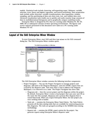
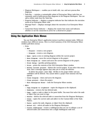
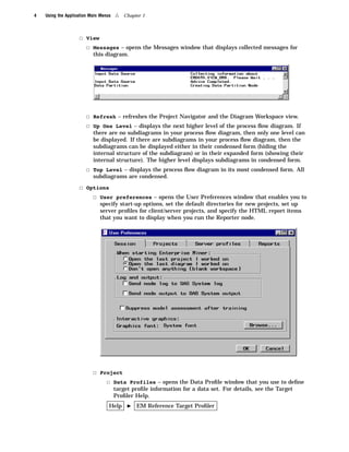
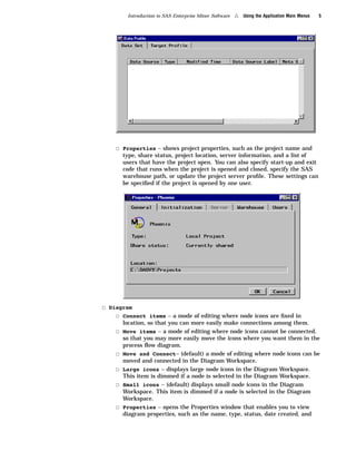
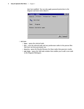
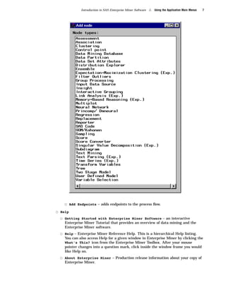
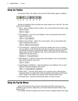
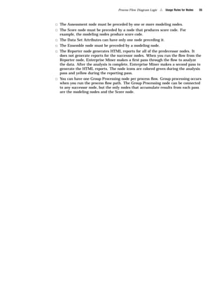
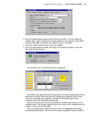
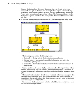
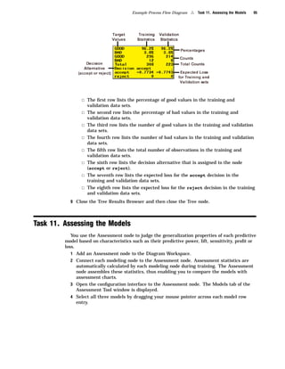
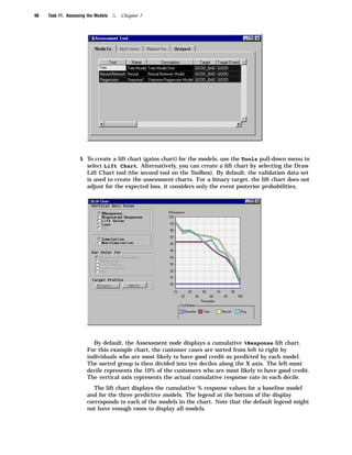
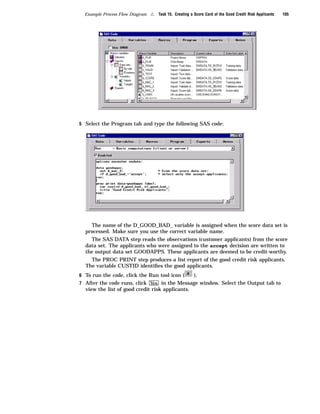
Getting Started with
SAS Enterprise Miner 4.3
® ™

The correct bibliographic citation for this manual is as follows: SAS Institute Inc. 2004.
Getting Started with SAS ® Enterprise Miner TM 4.3. Cary, NC: SAS Institute Inc.
Getting Started with SAS® Enterprise MinerTM 4.3
Copyright © 2004, SAS Institute Inc., Cary, NC, USA
ISBN 1-59047-231-4
All rights reserved. Produced in the United States of America. No part of this publication
may be reproduced, stored in a retrieval system, or transmitted, in any form or by any
means, electronic, mechanical, photocopying, or otherwise, without the prior written
permission of the publisher, SAS Institute Inc.
U.S. Government Restricted Rights Notice. Use, duplication, or disclosure of this
software and related documentation by the U.S. government is subject to the Agreement
with SAS Institute and the restrictions set forth in FAR 52.227–19 Commercial Computer
Software-Restricted Rights (June 1987).
SAS Institute Inc., SAS Campus Drive, Cary, North Carolina 27513.
1st printing, January 2004
SAS Publishing provides a complete selection of books and electronic products to help
customers use SAS software to its fullest potential. For more information about our
e-books, e-learning products, CDs, and hard-copy books, visit the SAS Publishing Web site
at support.sas.com/pubs or call 1-800-727-3228.
SAS® and all other SAS Institute Inc. product or service names are registered trademarks
or trademarks of SAS Institute Inc. in the USA and other countries. ® indicates USA
registration.
Other brand and product names are registered trademarks or trademarks of their
respective companies.

Contents

Chapter 1 4 Introduction to SAS Enterprise Miner Software 1
Data Mining Overview 1
Layout of the SAS Enterprise Miner Window 2
Using the Application Main Menus 3
Using the Toolbox 8
Using the Pop-Up Menus 8
Unavailable and Dimmed Items 9
Enterprise Miner Documentation 9

Chapter 2 4 Working with Projects 11
Project Overview 11
Project Directory Structure 12
Viewing and Specifying Project Properties 13
Creating a New Local Project 16
Creating a Client/Server Project 17
Opening a Process Flow Diagram 25
Opening an Existing Project 26
Saving a Project Diagram 27
Running a Project Diagram 27
Closing Projects and Diagrams 28
Creating a New Diagram 28
Deleting Projects and Diagrams 28
Project Troubleshooting Tips 29
Exporting Enterprise Miner 4.3 Projects 30
Opening Enterprise Miner Release 4.2 and Earlier Projects 30

Chapter 3 4 Building Process Flow Diagrams 33
Components Used to Build Process Flow Diagrams 33
Using the Diagram Workspace Pop-up Menu 35
Adding Nodes to a Diagram 35
Using the Node Pop-up Menu 36
Connecting Nodes in a Diagram 37
Cutting Connections in a Diagram 38
Deleting Nodes from a Diagram 39
Moving Nodes in a Diagram 40
Copying and Pasting a Node 40
Cloning a Node 40

Chapter 4 4 Process Flow Diagram Logic 43
Organization of Enterprise Miner Nodes 43
Sampling Nodes 44

iv

Exploring Nodes 45
Modifying Nodes 46
Modeling Nodes 47
Assessing Nodes 48
Scoring Nodes 48
Utility Nodes 49
Subdiagrams 50
Usage Rules for Nodes 54

Chapter 5 4 Common Features among Nodes 57
Functionality 57
Data Tab 57
Variables Tab 58
Notes Tab 60
Results Browser 60
Viewing and Setting Node Defaults 60

Chapter 6 4 Data Structure Examples 63
Types of Data Structures 63
Regression Data 64
Association Discovery Data 66

Chapter 7 4 Example Process Flow Diagram 69
Process Flow Diagram Scenario 69
Task 1. Creating a New Local Project 72
Task 2. Defining the Input Data Set 73
Task 3. Setting the Target Variable 74
Task 4. Defining a Target Profile for the GOOD_BAD Target Variable 74
Task 5. Examining Summary Statistics for the Interval and Class Variables 79
Task 6. Creating Training and Validation Data Sets 79
Task 7. Creating Variable Transformations 81
Task 8. Creating a Stepwise Logistic Regression Model 84
Task 9. Creating a Multilayer Perceptron Neural Network Model 87
Task 10. Creating a Tree Model 92
Task 11. Assessing the Models 95
Task 12. Defining the Score Data Set 98
Task 13. Scoring the Score Data Set 99
Task 14. Viewing the Expected Losses in the Score Data Set 100
Task 15. Creating a Score Card of the Good Credit Risk Applicants 104
Task 16. Closing the Diagram 106

Appendix 1 4 References 107
References 107

Appendix 2 4 Variable Layout for SAMPSIO.DMAGECR (German Credit Data Set) 109
SAMPSIO.DMAGECR (German Credit Data Set) 109

Appendix 3 4 Recommended Reading 111
Recommended Reading 111

Glossary 113
Index 123

1

CHAPTER

1
Introduction to SAS Enterprise
Miner Software

Data Mining Overview 1
Layout of the SAS Enterprise Miner Window 2
Using the Application Main Menus 3
Using the Toolbox 8
Using the Pop-Up Menus 8
Unavailable and Dimmed Items 9
Enterprise Miner Documentation 9

Data Mining Overview
SAS defines data mining as the process of uncovering hidden patterns in large
amounts of data. Many industries use data mining to address business problems and
opportunities such as fraud detection, risk and affinity analyses, database marketing,
householding, customer churn, bankruptcy prediction, and portfolio analysis.The SAS
data mining process is summarized in the acronym SEMMA, which stands for
sampling, exploring, modifying, modeling, and assessing data.
3 Sample the data by creating one or more data tables. The sample should be large
enough to contain the significant information, yet small enough to process.
3 Explore the data by searching for anticipated relationships, unanticipated trends,
and anomalies in order to gain understanding and ideas.
3 Modify the data by creating, selecting, and transforming the variables to focus the
model selection process.
3 Model the data by using the analytical tools to search for a combination of the
data that reliably predicts a desired outcome.
3 Assess the data by evaluating the usefulness and reliability of the findings from
the data mining process.
You might not include all of these steps in your analysis, and it might be necessary to
repeat one or more of the steps several times before you are satisfied with the results.
After you have completed the assessment phase of the SEMMA process, you apply the
scoring formula from one or more champion models to new data that might or might not
contain the target. The goal of most data mining tasks is to apply models that are
constructed using training and validation data to make accurate predictions about
observations of new, raw data.
The SEMMA data mining process is driven by a process flow diagram, which you can
modify and save. The GUI is designed in such a way that the business analyst who has
little statistical expertise can navigate through the data mining methodology, while the
quantitative expert can go “behind the scenes” to fine-tune the analytical process.
Enterprise Miner contains a collection of sophisticated analysis tools that have a
common user-friendly interface that you can use to create and compare multiple

2 Layout of the SAS Enterprise Miner Window 4 Chapter 1

models. Statistical tools include clustering, self-organizing maps / Kohonen, variable
selection, trees, linear and logistic regression, and neural networking. Data preparation
tools include outlier detection, variable transformations, data imputation, random
sampling, and the partitioning of data sets (into train, test, and validate data sets).
Advanced visualization tools enable you to quickly and easily examine large amounts of
data in multidimensional histograms and to graphically compare modeling results.
Enterprise Miner is designed for PCs that are running under Windows 95, 98, NT,
2000, XP, or subsequent releases of those operating environments. The figures and
screen captures presented in this document were taken on a PC running under
Windows NT 4.0.

Layout of the SAS Enterprise Miner Window
To start Enterprise Miner, start SAS and then type miner on the SAS command
dialog bar. The SAS Enterprise Miner window opens:

The SAS Enterprise Miner window contains the following interface components:
3 Project Navigator — You use the Project Navigator to manage projects and
diagrams, add tools to the Diagram Workspace, and view HTML reports that are
created by the Reporter node. Note that when a tool is added to the Diagram
Workspace, it is referred to as a node. The Project Navigator has three tabs:
3 Diagrams tab — lists the current project and the diagrams within the project.
By default, Enterprise Miner creates a local project that uses your user ID as
the name (for this example, Phoenix) and a process flow diagram that is
named Untitled. When you reopen Enterprise Miner, the last project you
were working with is loaded.
3 Tools tab — contains the Enterprise Miner Tools Palette. The Tools Palette
presents all the data mining tools that are available for constructing process
flow diagrams. The tools are grouped according to the SEMMA data mining
methodology.
3 Reports tab — contains the HTML report entries for the project. You
generate reports using Enterprise Miner’s Reporter node.

Introduction to SAS Enterprise Miner Software 4 Using the Application Main Menus 3

3 Diagram Workspace — enables you to build, edit, run, and save process flow
diagrams.
3 Tools Bar — contains a customizable subset of Enterpriser Miner tools that are
commonly used to build process flow diagrams in the Diagram Workspace. You can
add or delete tools from the Tools Bar.
3 Progress Indicator — displays a progress indicator bar that indicates the execution
status of an Enterprise Miner task.
3 Message Panel — displays messages about the execution of an Enterprise Miner
task.
3 Connection Status Indicator — displays the remote host name and indicates
whether or not the connection is active for a client/server project.

Using the Application Main Menus
You use Enterprise Miner’s application menus to perform common tasks. Different
windows have different menus. Here is a brief summary of the SAS Enterprise Miner
window pull-down menus:
3 File
3 New
3 Project – creates a new project.
3 Diagram – creates a new diagram.
3 Open – opens a new or existing diagram within the current project.
3 Save Diagram – saves the current diagram to the project.
3 Save Diagram as – names and saves the current diagram to the project.
3 Print Setup – specifies printing options.
3 Print – prints the contents of the SAS Enterprise Miner window.
3 Delete current project – deletes the current project. If you select this menu
item, then a message appears that asks you to verify the deletion.
To delete the project, select Yes . All files in the project folder and any
subfolders will be deleted. You cannot delete a project that someone else has
opened.
3 Close diagram – closes and saves the diagram.
3 Close project – closes the project.
3 Exit Enterprise Miner – ends the Enterprise Miner session.
3 Edit
3 Copy diagram to clipboard – copies the diagram to the clipboard.
3 Undelete – restores the last deleted node.
3 Copy – copies a node or object to the paste buffer. You must first select the node
or object that you want to copy.
3 Delete – deletes the selected node or connection from the Diagram Workspace.
3 Clone – copies the current node and adds it to the Custom folder of the Tools
Palette.
3 Paste – pastes the node, diagram, or object from the clipboard.
3 Select all – selects all nodes in the Diagram Workspace.
3 Create subdiagram – creates a subdiagram that you use to collapse a set of
selected nodes and connections into a single Subdiagram node icon.

4 Using the Application Main Menus 4 Chapter 1

3 View
3 Messages – opens the Messages window that displays collected messages for
this diagram.

3 Refresh – refreshes the Project Navigator and the Diagram Workspace view.
3 Up One Level – displays the next higher level of the process flow diagram. If
there are no subdiagrams in your process flow diagram, then only one level can
be displayed. If there are subdiagrams in your process flow diagram, then the
subdiagrams can be displayed either in their condensed form (hiding the
internal structure of the subdiagram) or in their expanded form (showing their
internal structure). The higher level displays subdiagrams in condensed form.
3 Top Level – displays the process flow diagram in its most condensed form. All
subdiagrams are condensed.
3 Options
3 User preferences – opens the User Preferences window that enables you to
specify start-up options, set the default directories for new projects, set up
server profiles for client/server projects, and specify the HTML report items
that you want to display when you run the Reporter node.

3 Project
3 Data Profiles – opens the Data Profile window that you use to define
target profile information for a data set. For details, see the Target
Profiler Help.
Help I EM Reference Target Profiler


3 Properties – shows project properties, such as the project name and
type, share status, project location, server information, and a list of
users that have the project open. You can also specify start-up and exit
code that runs when the project is opened and closed, specify the SAS
warehouse path, or update the project server profile. These settings can
be specified if the project is opened by one user.

3 Diagram
3 Connect items – a mode of editing where node icons are fixed in
location, so that you can more easily make connections among them.
3 Move items – a mode of editing where node icons cannot be connected,
so that you may more easily move the icons where you want them in the
process flow diagram.
3 Move and Connect– (default) a mode of editing where node icons can be
moved and connected in the Diagram Workspace.
3 Large icons – displays large node icons in the Diagram Workspace.
This item is dimmed if a node is selected in the Diagram Workspace.
3 Small icons – (default) displays small node icons in the Diagram
Workspace. This item is dimmed if a node is selected in the Diagram
Workspace.
3 Properties – opens the Properties window that enables you to view
diagram properties, such as the name, type, status, date created, and

6 Using the Application Main Menus 4 Chapter 1

date last modiﬁed. You can also apply password protection to the
diagram and store notes about it.

3 Actions
3 Open – opens the selected node.
3 Run – runs the selected node and any predecessor nodes in the process ﬂow
that have not been previously run.
3 Results– opens the Results Browser for those nodes that generate results.
3 Add Node – opens the Add node window that enables you to add a new node
to the Diagram Workspace.


3 Add Endpoints – adds endpoints to the process ﬂow.
3 Help
3 Getting Started with Enterprise Miner Software – an interactive
Enterprise Miner Tutorial that provides an overview of data mining and the
Enterprise Miner software.
3 Help – Enterprise Miner Reference Help. This is a hierarchical Help listing.
You can also access Help for a given window in Enterprise Miner by clicking the
What’s This? icon from the Enterprise Miner Toolbox. After your mouse
pointer changes into a question mark, click inside the window frame you would
like Help on.
3 About Enterprise Miner – Production release information about your copy of
Enterprise Miner.

8 Using the Toolbox 4 Chapter 1

Using the Toolbox
In Enterprise Miner, the toolbox at the top of the SAS window appears as follows:

Tool tips are displayed when you hold your mouse pointer over a tool icon. The icons
represent the following:
1 Open – opens a diagram within a project. You can also perform this task by using
the main menu:
File I Open

2 Save Diagram – saves the current diagram. You can also perform this task by
using the main menu
File I Save diagram

3 Delete Current Project – deletes the current project. You can also perform this
task by using the main menu:
File I Delete current project

4 User Preferences – opens the User Preferences window that you use to specify
start-up options, set the default directories for new projects, set up server proﬁles
for client/server projects, and specify the HTML report items that you want to
display when you run the Reporter node. You can also open the User Preferences
window from the main menu:
Options I User preferences

5 Print Diagram – prints the current process ﬂow diagram. You can also perform
this task by using the main menu:
File I Print

6 Copy Diagram to Clipboard – copies the diagram to the clipboard. You can also
perform this task by using the main menu:
Edit I Copy diagram to clipboard

7 What’s This? – turns the mouse pointer into a question mark, indicating that
Enterprise Miner is in Help mode. Click the question mark inside an Enterprise
Miner window to get Help on the contents of the selected window frame.
8 Getting Started – launches the Enterprise Miner 4.3 online tutorial.

Using the Pop-Up Menus
Many of the functions that are found in the Enterprise Miner main menus are
available in pop-up menus. Right-click a GUI object within Enterprise Miner to get
pop-up menus.
For example, instead of using the main menu to insert a diagram, follow these steps:

Introduction to SAS Enterprise Miner Software 4 Enterprise Miner Documentation 9

1 Select the Diagrams tab of the Project Navigator and right-click either the Project
folder, the diagram icon, or anywhere in the background of the tab. A pop-up
menu appears.
2 Select the New Diagram pop-up menu item. A new diagram is added to the project.

Unavailable and Dimmed Items
At times particular window objects and menu items are unavailable for use. When a
window object or menu item is unavailable, it appears dimmed and does not respond to
mouse clicks. When the data mining settings are changed so that the object’s use is
contextually appropriate, then the objects become active and will accept user input.
When you configure statistical settings within a node, dimmed objects prevent you
from selecting inappropriate option combinations. Selecting some options enables
additional option settings that you should specify to completely configure your data
mining node.

Enterprise Miner Documentation
For more information, see
3 Enterprise Miner Reference Help – describes how to use each Enterprise Miner
node as well as other features of Enterprise Miner, such as the Target Profiler.
Help is available through the Enterprise Miner main menu:
Help I EM Reference

Note: You can search for text strings in the EM Reference Help, using the menu
choices:
Edit I Find

and typing in a search string. 4
3 Frame Help – Enterprise Miner nodes have Help available at the window frame
level. For Help on a field or object that is contained in a particular window frame:
1 Click the What’s This? tool icon in the Enterprise Miner Toolbox. The
mouse pointer changes into a question mark.
2 Click inside the window that you would like help on.
3 Add-In Tools for SAS/Warehouse Administrator Software – To download
information about these tools, go to the SAS/Warehouse Administrator product
page: http://support.sas.com/rnd.
3 Data Mining Using SAS Enterprise Miner: A Case Study Approach, Second
Edition – provides simple directions about how to begin accessing data and how to
complete an analysis.

11

CHAPTER

2
Working with Projects

Project Overview 11
Project Directory Structure 12
Project Location 12
EMDATA Directory 13
EMPROJ Directory 13
REPORTS Directory 13
Viewing and Specifying Project Properties 13
Creating a New Local Project 16
Creating a Client/Server Project 17
Defining a New Server Profile 18
How to Create a Client/Server Project 22
Using a Server Profile in Batch Mode to Connect to a Server 25
Opening a Process Flow Diagram 25
Opening an Existing Project 26
Saving a Project Diagram 27
Running a Project Diagram 27
Closing Projects and Diagrams 28
Creating a New Diagram 28
Deleting Projects and Diagrams 28
Project Troubleshooting Tips 29
Exporting Enterprise Miner 4.3 Projects 30
Opening Enterprise Miner Release 4.2 and Earlier Projects 30

Project Overview
A project is a collection of Enterprise Miner process flow diagrams and information
that pertains to them. Projects are often differentiated by the type of data that you
intend to analyze. In other words, it is a good idea to create a separate project for each
major data mining problem that you intend to investigate. Local projects are useful
when the data is available locally on your machine. If you need to access databases on
a remote host or distribute the data-intensive processing to a more powerful remote
host, then you should create a client/server project.
Both local projects and client/server projects are shareable; that is, multiple users
can work on the same project simultaneously. In order for the project to be shareable,
all parties must access the same client files. The server.cfg client file uses the remote
server path to point to the server, allowing multiple users to work on the same project
on both the client and server side.
Although projects are shareable, only one user can open a diagram at a time. Users
can create, edit, and delete diagrams without affecting the work of others who are
sharing that project, because each diagram is an independent unit. Node clones and

12 Project Directory Structure 4 Chapter 2

target profiles that were created by one user may be shared by other users for use in
their own diagrams.
Updates to the project start-up or exit code, warehouse path, or server profile can be
made only when there is one and only one person using the project. To learn about how
to update these project settings, see “Viewing and Specifying Project Properties” on
page 13. In a shared environment, it may be necessary to request everyone to close that
project from within their own Enterprise Miner sessions, while an administrator makes
the required changes. The same applies to renaming or deleting a project.
In an Enterprise Miner client/server project, the server profile is stored with the
project, and is thus shared by all users of that project. Storing the profile with the
project facilitates profile maintenance in a shared project environment.

Project Directory Structure
For each project, Enterprise Miner dynamically creates a number of subdirectories
that have the following structure:

Note: To view your project files in a Windows file browser, select the Diagrams tab
of the Enterprise Miner Project Navigator, right-click a named project icon, and then
select Explore. 4
When you create a project, Enterprise Miner automatically assigns the EMDATA and
EMPROJ librefs to the EMDATA and EMPROJ subdirectories, respectively. Enterprise
Miner uses a standard directory structure and stores a given project’s files in the root of
the project directory. This enables you to back up or copy Enterprise Miner projects
simply by placing a copy of the project directory and its subdirectories in the new
location. Enterprise Miner does not limit the number of projects. There is a limit of
100,000 diagrams per project.

Project Location
The project location directory contains the .dmp file that corresponds to the project
definition, and the various .dmd files which represent the various diagrams that were
created within the project. The name of the .dmp file defines the name of the project.
The following display shows the directory layout for a project named Phoenix.

Working with Projects 4 Viewing and Specifying Project Properties 13

This project contains a diagram named My diagram.dmd.

EMDATA Directory
The EMDATA directory contains potentially large files that are created when you run
the process flows in your project. When you are running a project in client/server mode,
files are written to the server data directory instead. However, samples taken from the
remote location are stored in your EMDATA directory so you can continue to work when
a connection to the server is unavailable.

EMPROJ Directory
Project files that contain information for each diagram and its nodes, the target
profiler, and various registries are stored in the EMPROJ directory. Diagram lock (.lck)
files are also placed in the EMPROJ directory every time a diagram is opened. This
prevents two users from opening the same diagram at the same time. The name of the
lock file is always identical to the name of the diagram in question, except for the .lck
extension. For example, a diagram file that is named My diagram.dmd has a
corresponding My diagram.lck lock file.
The USERS subdirectory contains files that represent the users currently sharing the
project.

REPORTS Directory
HTML reports generated by the Reporter node are stored in this directory. Each
report has its own subdirectory. The name of the subdirectory defines the name of the
report.

Viewing and Specifying Project Properties
To view and customize properties for a project, use the main menu to select
Options I Project I Properties

The Properties window opens. The properties window contains five tabs:
3 General — displays the project name, type, share status, and location.

14 Viewing and Specifying Project Properties 4 Chapter 2

3 Initialization — speciﬁes whether to run start-up code (such as, assigning librefs
to data sources for the project or specifying the format search paths via the
FMTSEARCH option) when the project is opened, and exit code (such as clearing
libref assignments and resetting global SAS options) when the project is closed.

By default, start-up and exit code are enabled. To prevent either the start-up or
exit code from running, deselect the appropriate check box. These options appear
dimmed if the project is currently shared.
To deﬁne start-up or exit code, select Edit and type the code in the editor.

After entering your start-up code, close the window and save your changes.

Working with Projects 4 Viewing and Specifying Project Properties 15

3 Server — enables you to view and configure a default server profile. A server
profile contains all the configuration information that is necessary to establish a
connection on a remote server. You may edit the project server profile only when
no one else is using the project. For details about this task, see “Creating a Client/
Server Project” on page 17. Note that the Server tab is dimmed unless you are
viewing the properties for a client/server project.

3 Warehouse — enables you to type the warehouse path where the metadata sample
was created from the Enterprise Miner Add-ins to the SAS/Warehouse
Administrator. Alternatively, you can select Browse to find and set the warehouse
path via an explorer interface.

3 Users — lists the user ID and sign-on time for all of the users who currently have
the project open.

16 Creating a New Local Project 4 Chapter 2

After you have set the project properties, select OK in the Properties window or
select Cancel to cancel your settings.

Creating a New Local Project

To create a new local project:
1 From the File pull-down menu, select
New I Project

The Create New Project window opens:

Note: To reset the default directory for new projects, use the Options pull-down
menu to select User preferences. Select the Directory tab of the User
Preferences window and specify the default directory path for new projects.4
2 Type the location where you want the project to be stored in the Location ﬁeld.
You can also select Browse to browse through the folders on your machine and set
the project Location via an explorer interface.
3 Type the project name in the Name entry ﬁeld.

Working with Projects 4 Creating a Client/Server Project 17

4 To create the project, select OK . Enterprise Miner creates the project directories,
and then loads the project as the active project in the SAS Enterprise Miner
window. The project contains a default diagram named Untitled.

Creating a Client/Server Project
Enterprise Miner enables you to access data sources (such as SAS data sets or
database management systems) on a server to use with your local SAS Enterprise
Miner session. SAS/CONNECT is the cooperative processing software that establishes
the client/server connection between the remote and local hosts. For details, see the
SAS/CONNECT User’s Guide.
The client/server functionality provides the following advantages:
3 distributes data-intensive processing to the most appropriate machine
3 minimizes network traffic by processing the data on the server machine
3 minimizes data redundancy by maintaining one central data source
3 enables you to toggle between remote and local processing.
Defining a client/server project consists of two basic steps, which are accomplished
via a project wizard:
1 Define the client location for the project by providing the name and a location for
the project.
2 Provide a server profile. You can specify an existing profile or create a new profile.

18 Defining a New Server Profile 4 Chapter 2

Note: To use data sets that have user-defined formats on the server, you must
ensure that the formats are available both locally and on the server. At the client,
assign a format search path in a project’s start-up code. At the server, use the server
seed code to point to the format catalogs that reside on both the client and server. 4

Defining a New Server Profile
Before you define the location and name for the client/server project, you might want
to define a new server profile as part of your user preferences. A server profile contains
all of the information that is necessary to establish a connection to the remote server.
To define a new server profile, follow these steps:
1 Use the Options pull-down menu from the SAS Enterprise Miner window to select
the User Preferences item.
The User Preferences window opens. You define the server profile in the Server
profiles tab. This tab lists the current server profile directory and all of the profiles
that are stored in this directory. By default, server profiles are stored in the
SASUSER folder where Enterprise Miner was installed. To set the profile
directory, select Browse to find and set the directory.

2 To create a new profile, select New profile . A new profile entry that is named
Untitled is added to the list of server profiles. You can highlight the new profile
to select it and type in a new name, such as Gold Digger.

Working with Projects 4 Defining a New Server Profile 19

Note: To edit an existing profile, click Edit . To rename a profile, right-click on
the server profile in the list and select Rename. Type the profile name. To delete a
4
profile, click Delete .
3 Type a more descriptive profile name.
4 Click Edit . The Edit a Server Profile window opens.

Note: To load the profile settings from an existing profile, select Load profile .
Select the *.srv file that contains the profile settings for the existing server. 4
5 Type the remote host address name. The Host can be the machine name (for
example, golddigger.pc.sas.com) or its numeric IP address (123.321.12.99). The
address name for a NETBIOS network can contain a maximum of eight characters.
6 Select the drop-down arrow to set the Comamid parameter. The Comamid
parameter identifies the communication access method that is used to connect to
the remote host.
7 If a spawner is necessary to establish the remote connection, then type the share
port that the agent spawner runs on. You can type either the service name (for
example , shr3) or the port number (for example, 5012). The Port field is required
if you are running a Windows NT server where the agent spawner has been set up
to run on the share port. It is not required on other platforms.
8 Type the Default remote data path where Enterprise Miner will store large
intermediate files on the server. The path should be specified according to the host
machine’s naming convention. The server must be able to reference this location,

20 Defining a New Server Profile 4 Chapter 2

and you must have write access to this path. Files in this path are accessed via
remote library services when needed; they are not moved to the client.

9 Set the sign on script file. If Comamid is set to TCP, then you must set the script
file that is used to initiate and terminate the remote session. A script file is an
external file on the local system that contains special SAS statements that control
the connection. To set the script file, follow these steps:
a Select Signon script . The Signon Script window opens. At this stage, you can
open an existing script, or create a new one.
b To open an existing script, use the main menu commands:

File I Open

Alternatively, you can select the Open tool icon (third tool icon on the
toolbox). Find and select the script (.scr) file in the Open window and then
click Open . The script file is copied to the Signon Script window.
c To create a new script file, type the script file statements in the Signon Script
window or modify an existing script file. Save the script file by using the
File pull-down menu to select Save As.

d After you have set the script file, close the Signon Script window to return to
the Edit a Server Profile window.
10 If you need to enter start-up code that runs when the server is initialized, select
Start-up Code . The Start-up Code window opens. Type the start-up code in the
Start-up Code window. You do not need to enclose the statements in an RSUBMIT

Working with Projects 4 Defining a New Server Profile 21

block. You might want to use this feature to assign a libref to a remote directory
that contains SAS data sets via a LIBNAME statement or assign the SAS format
search path via the FMTSEARCH option. When you have finished entering your
start-up code, close the window. Your code is saved, and you return to the Edit a
Server Profile window.

11 To test the server profile, select Test signon .

The Test Result window opens, indicating whether Enterprise Miner was able to
establish a connection to the server.

If the connection failed, review the above steps to determine where you might
have incorrectly configured the server profile. You might want to consult your
systems administrator.
After you have configured the server profile, close the Edit a Server Profile window.
A message window opens that prompts you to save your changes to the server profile.
Select Yes to save your changes. Select No to prevent your changes from being saved
and to return to the SAS Enterprise Miner window. Select Cancel to return to the Edit
a Server Profile window.

22 How to Create a Client/Server Project 4 Chapter 2

How to Create a Client/Server Project
To create a client/server project, follow these steps:
1 Use the main menu to select

File I New I Project

The Create New Project window opens:

2 Type a name in for the project and select the Client/server project box. Use
the Location field to specify the path where you want to store your project files.
The path that you specify becomes the root of your project directory structure.

3 Select Create . The Client/server project window opens.
4 Specify an existing Server profile or create a new one.
3 To specify an existing server profile (a .srv file), use Browse to find and set
the server profile or type the server profile pathname. You can also define a
server profile in advance as part of the user preferences.

Working with Projects 4 How to Create a Client/Server Project 23

3 To create a new server profile, select New . Follow the steps outlined in
“Defining a New Server Profile” on page 18.

5 After you have defined the server profile, select OK to create the client/server
project.
6 A message window opens asking you if you want to connect to the server.

Select Yes to connect to the server or select No to run the project locally. The
project is automatically loaded as the active project in the SAS Enterprise Miner
window. The connection status indicator at the lower-right corner of the window
indicates whether the project is connected to the server.

To disconnect from the server, right-click on the project folder in the Project
Navigator and select Disconnect from server from the pop-up menu.

24 How to Create a Client/Server Project 4 Chapter 2

To connect to the server, right-click on the project folder in the Project Navigator and
select Connect to server from the pop-up menu.

Select Yes in the confirmation prompt window.

Note: You can also double-click on the connection status indicator to connect to the
server. 4
If you have an application that launches Enterprise Miner, but establishes a
connection beforehand, you can ensure that Enterprise Miner uses the existing
connection by editing the server.cfg file in your project’s EMPROJ subdirectory.

Type the CONID for the existing connection. For example, if your application
connects to a server using CONID=myhost, then you would type this value for the
CONID option in your server.cfg file. When you make these changes, Enterprise Miner
will not try to make a connection when opening the project if a connection already

Working with Projects 4 Opening a Process Flow Diagram 25

exists. If Enterprise Miner opens a project and uses an existing connection instead of
creating one, the connection is not terminated when you close the project.

Using a Server Profile in Batch Mode to Connect to a Server
You can use your server profile in batch mode to connect to the server by submitting
the following code from the SAS Program Editor window:
%let profile=c:profilesmy server.srv;
proc display c=sashelp.dmcon.connect.scl;
run;

Note: The code assumes that your server profile is named ’my server.srv’ and is
stored in c:profiles. You should modify those parameters to match the server profile
name and storage path with those on your installation. 4

Opening a Process Flow Diagram
To open a process flow diagram within the project:
1 Select the Diagrams tab of the Project Navigator if it is not already active.

2 Double-click on the diagram icon or label that you want to open. Alternatively, you
can right-click on the diagram label and select Open from the pop-up menu.

When a selected diagram is opened, the Diagram Workspace becomes active, and the
diagram can be edited, run, and saved. A diagram contains the data mining process
flow that you build interactively. You can think of a diagram as a type of graphical
computer program. For details about building process flow diagrams, see Chapter 3,
“Building Process Flow Diagrams,” on page 33.

Note: The fraud detection project contains one diagram named Untitled. You can
have more than one diagram for each project. 4

26 Opening an Existing Project 4 Chapter 2

Opening an Existing Project

To open an existing project or a diagram within that project, follow these steps:

File I Open

or you can just click the Open tool icon in the toolbox.
In the Open window, browse through the folders on your machine to find the
project .dmp file or the diagram .dmd file.

2 Select the project .dmp file or the diagram .dmd file that you want to open. If you
select a diagram .dmd file that is already opened by another user, then a message
window appears and indicates that the diagram is locked.
Select OK to open the project.
After you have opened a project, you must work with an existing diagram in the
project, create a new diagram, or wait until a locked diagram becomes available.
Note: Multiple users can open the same project (.dmp file) but not the same
diagram (.dmd file) within the project. 4
If the project is a client/server project, then a message window appears and asks if
you want to connect to the server.

Select Yes to establish a connection to the server or select No to run the project
locally.

Working with Projects 4 Running a Project Diagram 27

Saving a Project Diagram
To save a project diagram, first close any open nodes in the Diagram Workspace.
Then, use the File pull-down menu to select Save diagram.
File I Save diagram

Note that you can also perform this function by selecting the Save Diagram tool icon on
the Tools Bar.
To save the current diagram to a different name, use the File menu to select Save
diagram as. The Save Diagram As window opens. Type the diagram name in the Save
as field and then select OK .

Running a Project Diagram
To generate results from a process flow diagram, you must run the process flow path
to execute the code that is associated with each node. The paths can be run in several
ways:
3 When the node in the Diagram Workspace is closed and selected (a dotted line
surrounds selected nodes), you can use the main menu:
Actions I Run

3 Also if the node in the Diagram Workspace is closed, you can
1 Right-click the node to open a pop-up menu.
2 Select Run from the pop-up menu.
3 Many nodes, including all of the modeling nodes, can be run when the nodes’
tabbed configuration window is open. To run an open modeling node, select the
Run icon on the toolbox or use the main menu:
Tools I Train Model

For non-modeling nodes, select from the main menu
Tools I Run <Node Name>

You must run the predecessor nodes in your process flow diagram before you
can run an open node.
When a node in a process flow diagram is run, a green box surrounds each node icon
in succession as information is passed from node to node in the process flow. When you
run a process flow diagram that contains a Group Processing node, a blue box
surrounds the Group Processing node icon to indicate the beginning of each loop
iteration. If the process flow diagram contains a Reporter node, yellow boxes surround
the predecessor nodes to indicate that the HTML reports are being generated. Red
boxes surround nodes that fail when executed. To determine the error condition that is
associated with a failed node, use the main menu
View I Messages

In most cases, if you have not run the predecessor nodes in the process flow, then
these nodes automatically run when you run the selected successor node. If you have
already run the predecessor nodes in the process flow, and you have not changed any of
the node settings in the interim, then they do not run when you run the selected
successor node. Any nodes that follow the selected node are not run.

28 Closing Projects and Diagrams 4 Chapter 2

When the path has executed, a message dialog box appears and states that the task
is completed.
Select Yes to close the message dialog box.

You can view the results for nodes that generate results by right–clicking the node
icon in the process ﬂow diagram and selecting Results from the pop-up menu.
Alternatively, use the main menu:
Actions I Results

Closing Projects and Diagrams
To close a project that is open, right-click the project folder in the Project Navigator
and select Close. You can also use the main menu:
File I Close project

Both methods automatically save your changes to the project.
To close a diagram, use the main menu:
File I Close diagram

Creating a New Diagram
To create a new diagram, follow these steps:
1 Open the project that will contain the new diagram.
2 Right-click anywhere in the Diagram tab of the Project Navigator and select the
New Diagram.
3 By default, a new diagram named Untitled is added to the project. An n
subscript is added to the diagram name to distinguish untitled diagrams.
Alternatively, you can use the main menu:
File I New I Diagram

The diagram becomes active in the Diagram Workspace. To rename the diagram,
right-click on the diagram label in the Project Navigator and select Rename.

Deleting Projects and Diagrams
To delete a project, ﬁrst open the project to be deleted, then right-click on the project
name in the Project Navigator and select Delete current project.

Working with Projects 4 Project Troubleshooting Tips 29

Alternately, you could select the project name in the Project Navigator and use the
main menu:
File I Delete current project

A dialog box prompts you to verify the deletion.

CAUTION:
If you placed your own files within the project’s directory tree structure (for example, a
SAS data set), then these files are also deleted when you delete the project. All files
within the project folder are deleted! 4
Other ways to delete a project include the following:
3 Delete the root project directory from outside Enterprise Miner by using another
tool, such as Windows Explorer. In order to delete it from outside Enterprise Miner,
the project must not be open. You can delete only local projects with this method.

You can delete a project only if you are the sole user.
If you delete a client/server project when you have a connection to the server, then all
of the project files are deleted — including those on the remote host. If you have no
connection to the server, and choose not to reconnect, then only the local project files
are deleted. A local “kill” file named “projectname_kill.sas” is written to the project root
directory. When you submit this kill file from the SAS Program Editor window, a
connection is established to the server and then the project remote files are deleted.
To delete a diagram, right-click on the diagram name in the Project Navigator and
then select the Delete pop-up menu item. A dialog box prompts you to verify the
deletion.

Project Troubleshooting Tips
If an Enterprise Miner program fails or halts, then the .lck file for the diagram is not
usually deleted. The file will prevent you from reopening the diagram in a new

30 Exporting Enterprise Miner 4.3 Projects 4 Chapter 2

Enterprise Miner session, because you will hold a lock on the diagram. If this occurs,
follow these steps:
1 Close your Enterprise Miner session.
2 Use Windows Explorer or another file utility to locate and open the EMPROJ
subfolder for the project.
3 Find the .lck file that matches the diagram that you were working on and delete it.
4 Restart Enterprise Miner and open the diagram.

If you restart Enterprise Miner and the Project Properties window indicates the
project is currently being shared, but you know that you are the only person using the
project, then Enterprise Miner was also probably not shut down properly. In this case,
follow these steps:
1 Close all Enterprise Miner sessions.
2 Make sure that no one else is using the project.
3 Use Windows Explorer or another file utility to open the EMPROJ folder for the
project.
4 Open the USERS folder and delete its contents, but not delete the USERS folder.
5 Restart Enterprise Miner and reopen the project.

If you try to open a project and are informed by a message window that the project
libraries could not be assigned, then either the EMPROJ or EMDATA library is still in
use. A few reasons why the EMPROJ or EMDATA library is still in use include the
following:
3 An FSVIEW window for a data set in either library could be open.
3 A CATALOG window is open.
3 A data set or some other SAS file was not closed properly by Enterprise Miner.
You should first try to find and close the window that is using the data set or file. If
you are still unable to open the project, you should close and then restart Enterprise
Miner. If this step fails as well, then close and restart SAS.

Exporting Enterprise Miner 4.3 Projects
In Enterprise Miner 4.3, the project export wizard has been removed. Since
Enterprise Miner 3.x and 4.x projects are self-contained in the project root directory,
exporting a project simply involves copying or moving the entire project to the desired
target location using an external application such as Windows Explorer. You might also
want to use a third-party application such as Winzip to archive the project before
exporting it to a new location. You can unzip the project in your new directory.
For Enterprise Miner 3.x and 4.x client/server projects, you should archive the server
files separately from the client files.

Opening Enterprise Miner Release 4.2 and Earlier Projects
Enterprise Miner 4.3 runs on SAS 9.1, but can still open most Enterprise Miner
projects that were created in versions of Enterprise Miner that used SAS Versions 7
and 8. To open a project that was saved in Enterprise Miner 3.x, 4.0, 4.1, or 4.2, you
must convert the project files for use with SAS System 9.

Working with Projects 4 Opening Enterprise Miner Release 4.2 and Earlier Projects 31

CAUTION:
You should ALWAYS back up your legacy Enterprise Miner projects and data files before
attempting to convert them to Enterprise Miner 4.3 format! After you have converted your
Enterprise Miner projects to comply with SAS 9.1, you will not be able to reopen them in
earlier versions of Enterprise Miner. 4
To open a project from an Enterprise Miner 3.x, 4.1, or 4.2 release, follow these steps:
1 Back up the project file that you are preparing to convert and put it in a safe
location.
2 Invoke Enterprise Miner 4.3 and from the main menu, select
File I Open

3 Use the interface to locate the *.dmp project file from the prior release or version of
Enterprise Miner. In the legacy project directory, select the project and click Open .
4 A Conversion to SAS V9 Required window opens.

Note: Do not revisit converted project files using SAS Release 6.12, SAS
Versions 7 or 8 after the conversion. Attempts to add and delete diagrams will
corrupt the project file. If you want to use separate versions of Enterprise Miner
on the same project, you should make a copy of the project files to use with your
legacy version of Enterprise Miner, and use a different copy for conversion and use
in Enterprise Miner 4.3. 4
5 Select Yes and OK to proceed with the conversion.

33

CHAPTER

3
Building Process Flow Diagrams

Components Used to Build Process Flow Diagrams 33
The Tools Palette 34
The Tools Bar 34
The Messages Window 34
Using the Diagram Workspace Pop-up Menu 35
Adding Nodes to a Diagram 35
Using the Node Pop-up Menu 36
Connecting Nodes in a Diagram 37
Cutting Connections in a Diagram 38
Deleting Nodes from a Diagram 39
Moving Nodes in a Diagram 40
Copying and Pasting a Node 40
Cloning a Node 40

Components Used to Build Process Flow Diagrams
After opening a project diagram, you use the Diagram Workspace, the Tools Palette
of the Project Navigator, and the Tools Bar to edit and modify the diagram; that is, you
can add nodes, connect nodes, cut connections, and delete nodes.

The Tools Bar and the application main menus at the top of the SAS Enterprise
Miner window also contain useful items for constructing process ﬂow diagrams. For
details about using the Main Menus, see “Using the Application Main Menus” on page 3.

34 The Tools Palette 4 Chapter 3

The Tools Palette
The Tools Palette in the Project Navigator displays all of the data mining tools that
are available for constructing process flow diagrams. The tools are grouped according to
the phase of the SEMMA data mining process. You drag nodes from the Tools Palette
onto the Diagram Workspace.
To view the properties of a node, right-click on the tool icon and select the
Properties pop-up menu item. For details about this task, see “Viewing and Setting
Node Defaults” on page 60.
For a description of the nodes, see “Organization of Enterprise Miner Nodes” on page
43.

The Tools Bar
By default, the Tools Bar contains a subset of Enterprise Miner tools that are
commonly used to build process flow diagrams in the Diagram Workspace. You can also
drag tools from the Tools Bar onto the Diagram Workspace. To display tool tips, move
your mouse pointer slowly over the icons on the Tools Bar.
To reposition a tool on the Tools Bar, drag the tool icon to the desired location.
To add a node from the Tools Palette to the Tools Bar, drag the tool icon from the
Tools Palette to the Tools Bar.
To remove a tool from the Tools Bar, right-click on the tool icon and select Remove
from tool bar.
To view the properties for a tool, right-click on a tool icon and select Tool
Properties.

The Messages Window
The Messages window displays messages that are generated by the creation or
execution of a process flow diagram. The Messages window is useful for detecting errors
that might have occurred when you were running a node or a process flow path. To
display the Messages window, use the View pull-down menu to select Messages. The
Messages window appears. You must close the Messages window to continue working
with the process flow diagram.

Building Process Flow Diagrams 4 Adding Nodes to a Diagram 35

The messages are stored as part of the diagram. They can be cleared from within the
Messages window by selecting from the main menu:
Edit I Clear Text

Note: Messages are also displayed in the message panel when you create or execute
a process flow diagram. 4

Using the Diagram Workspace Pop-up Menu
You can use the Diagram Workspace pop-up menus to perform many tasks. To open
the pop-up menu, right-click in an open area of the Diagram Workspace. (Note that you
can also perform many of these tasks by using the pull-down menus.) The pop-up menu
contains the following items:
3 Add node — accesses the Add Node window.
3 Add endpoints — adds enter and exit endpoints to a subdiagram.
3 Paste — pastes a node from the clipboard to the Diagram Workspace.
3 Undelete — undeletes the last deleted node.
3 Delete — deletes the selected node.
3 Select All — selects all nodes in the process flow diagram.
3 Create subdiagram — creates a subdiagram (see “Subdiagrams” on page 50). To
create a subdiagram, you must first select the nodes and connections that are to be
included in the subdiagram.
3 Refresh — refreshes the image that is displayed in the Enterprise Miner window.
3 Up one level — collapses a subdiagram.
3 Top level — moves to the top level of the process flow diagram. At the top level,
all subdiagrams are condensed.
3 Connect items — a mode of editing in which node icons are fixed in one location
so that it is easier to connect nodes.
3 Move items — a mode of editing in which node icons cannot be connected so that
it is easier to move nodes.
3 Move and connect — the default mode of editing in which node icons can be
moved and connected.

Adding Nodes to a Diagram
You add nodes to the Diagram Workspace to create a process flow. Nodes should be
connected in a logical order that represents the desired components of the sample,
explore, modify, model, and assess (SEMMA) methodology.
You can add nodes to a process flow diagram in several ways:
3 Drag node icons from the Tools Palette of the Project Navigator to the Diagram
Workspace.
3 Drag node icons from the Tools Bar to the Diagram Workspace. This task is
accomplished the same way that you drag nodes from the Tools Palette.
3 Use the Diagram Workspace pop-up menu. Right-click on an open area in the
Diagram Workspace, and select Add node. The Add Node window appears.

36 Using the Node Pop-up Menu 4 Chapter 3

Select a node from the list. The node appears in the Diagram Workspace.
3 Double-click an open area in the Diagram Workspace to display the Add Node
window.
3 Use the Actions main menu to select the Add Node menu item. This action opens
the Add Node window.

Using the Node Pop-up Menu
To open a node pop-up menu, right-click on a node icon in the Diagram Workspace.
The node pop-up menu contains the following items:
3 Open — opens the node.
3 Run — runs both the selected node and all predecessor nodes in the process ﬂow
diagram that have not been run.
3 Results — opens the node Results Browser for those nodes that generate results.
You must run the node before you can open the Results Browser.
3 Copy — copies the node to the paste buffer.
Note: To paste the node onto the Diagram Workspace, use the Edit pull-down
menu to select the Paste menu item.

Building Process Flow Diagrams 4 Connecting Nodes in a Diagram 37

3 Delete — deletes the node.
3 Clone — clones a node.
3 About — displays node properties in the About window.
3 Connect items — a mode of editing in which node icons are fixed in location so
that it is easier to connect nodes.
3 Move items — a mode of editing in which node icons cannot be connected so that
it is easier to move nodes.
3 Move and connect — the default mode of editing in which node icons can be
moved and connected.

Connecting Nodes in a Diagram
You connect nodes in the Diagram Workspace to create a logical process flow. When
you create a process flow, you should follow the Sample, Explore, Modify, Model, and
Assess (SEMMA) data mining methodology. Information flows from node to node in the
direction that the connecting arrows point.

There are three editing modes available in the Diagram Workspace. You can right-click
on a node to access these modes.
3 Connect items — Create connections between nodes. In this editing mode, the
nodes are fixed in location, so that you can more easily make connections.
3 Move items — Move nodes from one location to another within the Diagram
Workspace. In this editing mode, you cannot make connections.
3 Move and connect — Move and Connect is the default mode for moving and
connecting items.
As an exercise in connecting nodes, connect the Input Data Source node to the
Sampling node. If the Input Data Source node is located to the left of the Sampling
node, the steps to create a connection are
1 Move the mouse pointer to the right edge of the Input Data Source icon. The
mouse pointer changes from an arrow to a cross.
2 Select and hold the left mouse button down, drag the mouse pointer to the left
edge of the Sampling node icon, and release the mouse button. A successful
connection results in a line segment that joins the two nodes.

38 Cutting Connections in a Diagram 4 Chapter 3

Note that if the Input Data Source icon moves (instead of making a connection),
then you should right-click on the node icon and select the Connect items pop-up
menu item. You can also move the mouse pointer away from the icons and
single-click the left mouse button, and then attempt to make the connection.
3 Move the mouse pointer away from the node icons, and click a blank area. The
line segment that connects the tool icon becomes an arrow, coming from the Input
Data Source node icon and pointing at the Sampling node icon. The direction of
the arrow is important because it indicates the direction of the information flow
from one node to the next. In this example, the Input Data Source node is the
predecessor node, and the Sampling node is the successor node in the process flow.

You use this same technique to connect additional nodes. Most nodes can have
multiple predecessor and successor nodes. See “Usage Rules for Nodes” on page 54 for
more information.

Cutting Connections in a Diagram
To cut a connection between two nodes:
1 Select the arrow that connects the nodes. The arrow changes to a line segment.

2 Allow the mouse pointer to remain on the line segment, and then right-click to
open a pop-up menu.
3 Select the Delete pop-up menu item. The line segment disappears from the
Diagram Workspace, and the nodes are no longer connected. Cutting the
connection between node icons cuts the information flow between those nodes.

Building Process Flow Diagrams 4 Deleting Nodes from a Diagram 39

Deleting Nodes from a Diagram
To delete a node from a process flow diagram:
1 Right-click on the node icon to open a pop-up menu.
2 Select the Delete pop-up menu item. A verification window appears that asks you
to verify that you want to delete this node. If you select OK , then the node is
removed from the process flow diagram. If you select Cancel , then the node
remains in the process flow diagram.
Note: This task can also be performed by selecting the node and using the Delete
tool icon from the toolbox. 4
To restore the deleted node, right-click in an open area of the Diagram Workspace
area and select the Undelete pop-up menu item. The node is copied to the Diagram
Workspace, but any previous connections are lost. You must redraw your node
connections.
To delete multiple nodes:
1 Select a node icon that you want to delete, and then SHIFT-click or CTRL-click
the remaining node icons that you want to delete. The selected nodes become
highlighted. Alternatively, you can select multiple nodes by dragging your mouse
pointer around the nodes that you want to delete. A box appears around the
selected node icons. This technique is referred to as “rubber banding” nodes.
2 Allow the mouse pointer to remain on the selected icons, and then right–click to
open a pop-up menu.
3 Select the Delete pop-up menu item. A verification window appears that asks you
to verify that you want to delete these nodes. If you select OK , then the nodes
and their connections are removed from the process flow diagram. If you select
Cancel , then the nodes remain in the process flow diagram.

To delete all nodes in the process flow diagram:
1 From the main menu, select
Edit I Select all

2 After all the nodes are selected, from the main menu select
Edit I Delete

or click the Delete icon from the toolbox.
Note: You cannot restore a multiple-node deletion. 4
When you delete a predecessor node in a process flow diagram, the results are still
available in the successor node or nodes. It is important to note that the results may
not be reliable or accurate. For example, assume that you defined the following process
flow diagram and ran the flow from the Regression node:

You then decide to delete the existing Data Partition node and add a new Data
Partition node to the flow. The Regression node will still store the results from the first

40 Moving Nodes in a Diagram 4 Chapter 3

run of the flow. To obtain the updated regression results, you need to re-run the entire
process flow diagram.

Moving Nodes in a Diagram
To move a node within a process flow diagram:
1 Use the mouse pointer to drag the node that you want to move. A box appears
around the icon to indicate that it has been selected.
2 Drag the node icon to a new position in the Diagram Workspace. Note that when
you drag the node icon, the mouse pointer becomes the shape of a hand. The
connection arrows will typically bend or stretch (or both) to accommodate the move.
Note: To move multiple nodes, select them all by using keyboard and mouse
combinations. CTRL-click to select multiple individual nodes that you want to move as
a group. 4

Copying and Pasting a Node
You can copy an existing node to memory and paste it in the Diagram Workspace.
The same node attributes that you copy are used in the new node. You can copy a node
from one diagram and paste it to another diagram if you want. However, you cannot
copy a node from one project to another project. To copy an existing node:
1 Right-click on the node that you want to copy in the Diagram Workspace. Select
the Copy pop-up menu item.
2 Right-click on the location where you want to paste the node. Select the Paste
pop-up menu item.
Because a Subdiagram node can represent multiple nodes in a diagram, you can use
the Subdiagram node to copy multiple nodes at one time.

Cloning a Node
You may want to clone a node if you plan to use the node repeatedly in a project. For
example, assume that you have defined an input data set in an Input Data Source node.
If you want to use the same input data set in the current diagram or in another
diagram of the project, then you can clone the existing Input Data Source node. When
you clone a node, it is added as a new node on the Tools Palette in the Custom section.
When you want to use the node, you simply drag it from the Tools Palette onto the
Diagram Workspace. The information that is contained in the original (parent) node is
included in the cloned node; for example, the target variable, the roles and
measurement levels for other variables and for the metadata sample are the same. You
can also redefine the attributes of the cloned node.
If you did not clone the node, you would have to add a new Input Data Source node
to the Diagram Workspace, set the node options, and create the metadata sample. If
you are going to use the same data set often in the project, then cloning an existing
node will save time.
Note: If you are going to use the same data set in several projects or diagrams, you
can use the SAS/Warehouse Administrator to set up the data sets, and use the

Building Process Flow Diagrams 4 Cloning a Node 41

Enterprise Miner add-in tools for applying whatever measurement levels and roles you
want in your data. Any users who use this data will pick up the metadata sample,
along with the roles and measurement levels that are already assigned. 4
To clone multiple nodes, condense the nodes into a subdiagram node (see
“Subdiagrams” on page 50) and then clone the subdiagram node.
To clone a node:
1 Select the node that you want to clone (the parent node) in the Diagram
Workspace.
2 Right–click the node and select the Clone pop-menu item.
The Clone Current Node window opens.

The Clone Current Node window lists the selected node and the following new
tool (node) information:
3 Cloned data — the SAS entry that contains the new node information.
3 Cloned class — the catalog entry that identiﬁes the parent node.
3 Description — the name of the cloned node. By default, the description is set
to Clone of node-name. You can type a new description in the entry ﬁeld if
you want.
3 Image — the icon that is used for the cloned node on the Tools Palette, Tools
Bar, and the Diagram Workspace. By default, the parent node icon is used as
the clone node icon. To change the icon image, select the arrow and then
select an icon from the list.
3 Type a node description. This example uses the default description Clone of
SAMPSIO.DMAGECR.
4 Select the Image arrow and then select a new icon.
5 Select OK to return to the Diagram Workspace.

The node is added as Clone of SAMPSIO.DMAGECR under the folder named Custom
in the Tools Palette of the Project Navigator.

42 Cloning a Node 4 Chapter 3

The cloned node (for this example, SAMPSIO.DMAGECR) can be used just like any
other node on the Tools Palette. It can be redefined and/or connected to other nodes in a
process flow, deleted, copied to the Tools Bar, and used in other process flow diagrams of
the project.
Note: If you are working in a shared project environment, you should periodically
refresh the Tools Palette in order to see and use clones that might have been created by
other users. 4

43

CHAPTER

4
Process Flow Diagram Logic

Organization of Enterprise Miner Nodes 43
Sampling Nodes 44
Exploring Nodes 45
Modifying Nodes 46
Modeling Nodes 47
Assessing Nodes 48
Scoring Nodes 48
Utility Nodes 49
Subdiagrams 50
Subdiagram Example 1 50
Subdiagram Example 2 52
Usage Rules for Nodes 54

Organization of Enterprise Miner Nodes
The nodes of Enterprise Miner are organized into categories of the Sample, Explore,
Modify, Model, and Assess (SEMMA) data mining methodology. In addition, there are
also Scoring and Utility node tools. You use the Scoring node tools to score your data
models and to create freestanding code. You use the Utility node tools to submit SAS
programming statements, to create data mining databases, to perform group processing,
to deﬁne control points in the process ﬂow diagram, and to create subdiagrams.
All of the Enterprise Miner nodes are listed in a set of folders that are located on the
Tools tab of the Enterprise Miner Project Navigator. The nodes are listed under the
folder that corresponds to their data mining functions.

44 Sampling Nodes 4 Chapter 4

Remember that in a data mining project, repeating parts of the data mining process
can offer advantages. For example, you may want to explore data and plot data at
several intervals throughout your project. It may be advantageous to fit models, assess
the models, and then refit the models and then assess them again.

Sampling Nodes

3 Use the Input Data Source node to access SAS data sets and other types of data.
This node reads data sources and defines their attributes for processing by
Enterprise Miner. Meta information (the metadata sample) is automatically
created for each variable when you import a data set with the Input Data Source

Process Flow Diagram Logic 4 Exploring Nodes 45

node. Initial values are set for the measurement level and the model role for each
variable. You can change these values if you are not satisfied with the automatic
selections that the node makes. Summary statistics are displayed for interval and
class variables.
3 Use the Sampling node to take random, stratified random samples, and to take
cluster samples of data sets. Sampling is recommended for extremely large
databases because it can significantly decrease model training time. If the random
sample sufficiently represents the source data set, then data relationships that
Enterprise Miner finds in the sample can be extrapolated upon the complete
source data set.The Sampling node writes the sampled observations to an output
data set and saves the seed values that are used to generate the random numbers
for the samples so that you may replicate the samples.
3 Use the Data Partition node to partition data sets into training, test, and
validation data sets. The training data set is used for preliminary model fitting.
The test data set is an additional hold-out data set that you can use for model
assessment. The validation data set is used to monitor and tune the model
weights during estimation and is also used for model assessment. This node uses
simple random sampling, stratified random sampling, or user defined partitions to
create partitioned data sets.

Exploring Nodes

3 The Distribution Explorer node is an advanced visualization tool that enables you
to quickly and easily explore large volumes of data in multidimensional
histograms. You can view the distribution of up to three variables at a time with
this node. When the variable is binary, nominal, or ordinal, you can select specific
values to exclude from the chart. To exclude extreme values for interval variables,
you can set a range cutoff. The node also generates summary statistics for the
charting variables.
3 The Multiplot node is another visualization tool that enables you to explore larger
volumes of data graphically. Unlike the Insight or Distribution Explorer nodes, the
Multiplot node automatically creates bar charts and scatter plots for the input and
target variables without requiring you to make several menu or window item
selections. The code that is created by this node can be used to create graphs in a
batch environment, whereas the Insight and Distribution Explorer nodes must be
run interactively.
3 Use the Insight node to open a SAS/INSIGHT session. SAS/INSIGHT software is
an interactive tool for data exploration and analysis. With it, you explore data
through graphs and analyses that are linked across multiple windows. You can
analyze univariate distributions, investigate multivariate distributions, and fit
explanatory models by using generalized linear models.
3 Use the Association node to identify association relationships within the data. For
example, if a customer buys a loaf of bread, how likely is the customer to also buy
a gallon of milk? You also use the Association node to perform sequence discovery
if a time stamp variable (a sequence variable) is present in the data set. Binary
sequences are constructed automatically, but you can use the Event Chain
Handler to construct longer sequences that are based on the patterns that the
algorithm discovered.
3 You use the Variable Selection node to evaluate the importance of input variables
in predicting or classifying the target variable. To preselect the important inputs,
the Variable Selection node uses either an R-Square or a Chi-Square selection

46 Modifying Nodes 4 Chapter 4

(tree based) criterion. You can use the R-Square criterion to remove variables in
hierarchies, remove variables that have large percentages of missing values, and
remove class variables that are based on the number of unique values. The
variables that are not related to the target are set to a status of rejected.
Although rejected variables are passed to subsequent nodes in the process flow
diagram, these variables are not used as model inputs by a more detailed modeling
node, such as the Neural Network and Tree nodes. You can reassign the status of
the input model variables to rejected in the Variable Selection node.
3 Use the Link Analysis node to transform data from differing sources into a data
model that can be graphed. The data model supports simple statistical measures,
presents a simple interactive graph for basic analytical exploration, and generates
cluster scores from raw data that can be used for data reduction and segmentation.

Modifying Nodes

3 Use the Data Set Attributes node to modify data set attributes, such as data set
names, descriptions, and roles. You can also use the Data Set Attributes node to
modify the metadata sample that is associated with a data set, and to specify
target profiles for a target. An example of a useful Data Set Attributes application
is to generate a data set in the SAS Code node and then modify its metadata
sample with this node.
3 Use the Transform Variables node to transform variables. For example, you can
transform variables by taking the square root of a variable or by taking its natural
logarithm. Additionally, the Transform Variables node supports user-defined
formulas for transformations and provides a visual interface for grouping
interval-valued variables into buckets or quantiles. Transforming variables to
similar scale and variability may improve the fit of models, and subsequently, the
classification and prediction precision of fitted models.
3 Use the Filter Outliers node to identify and remove outliers or “noise” from data
sets. Checking for outliers is recommended as outliers may greatly affect modeling
results and, subsequently, the classification and prediction precision of fitted
models.
3 Use the Replacement node to impute (fill in) values for observations that have
missing values. You can replace missing values for interval variables with the
mean, median, midrange, or mid-minimum spacing, or with a distribution-based
replacement. Alternatively, you can use a replacement M-estimator such as Tukey’s
biweight, Huber’s, or Andrew’s Wave. You can also estimate the replacement
values for each interval input by using a tree-based imputation method. Missing
values for class variables can be replaced with the most frequently occurring
value, distribution-based replacement, tree-based imputation, or a constant.
3 Use the Clustering node to segment your data so that you can identify data
observations that are similar in some way. When displayed in a plot, observations
that are similar tend to be in the same cluster, and observations that are different
tend to be in different clusters. The cluster identifier for each observation can be
passed to other nodes for use as an input, ID, or target variable. It can also be
passed as a group variable that enables you to automatically construct separate
models for each group.
3 Use the SOM/Kohonen node to generate self-organizing maps, Kohonen networks,
and vector quantization networks. The SOM/Kohonen node performs unsupervised
learning in which it attempts to learn the structure of the data. As with the
Clustering node, after the network maps have been created, the characteristics can

Process Flow Diagram Logic 4 Modeling Nodes 47

be examined graphically by using the SOM/Kohonen Results Browser. The SOM/
Kohonen node provides the analysis results in the form of an interactive map that
illustrates the characteristics of the clusters. Furthermore, the SOM/Kohonen node
Results Browser provides a report that indicates the importance of each variable.
3 The Time Series experimental node converts transactional data to time series
data, and performs seasonal and trend analysis on an interval target variable.
3 Use the Interactive Grouping node to interactively group variable values into
classes. The Interactive Grouping functionality is required to create a specific type
of predictive model that is called a score card. Statistical and plotted information
can be interactively rearranged as you explore various variable groupings. Score
card models are frequently used for application and behavioral scoring in the
credit scoring industry.

Modeling Nodes

3 Use the Regression node to fit both linear and logistic regression models to your
data. You can use continuous, ordinal, and binary target variables. You can use
both continuous and discrete variables as inputs. The node supports the stepwise,
forward, and backward selection methods. A point-and-click interaction builder
enables you to create higher-order modeling terms.
3 Use the Tree node to fit decision tree models to your data. The implementation
includes features that are found in a variety of popular decision tree algorithms
(for example, CHAID, CART, C4.5, and C5.0.) The Tree node supports both
automatic and interactive training. When you run the Tree node in automatic
mode, it automatically ranks the input variables based on the strength of their
contribution to the tree. This ranking may be used to select variables for use in
subsequent modeling. You may override any automatic step with the option to
define a splitting rule and delete explicit nodes or subtrees. Interactive training
enables you to explore and evaluate a large set of trees as you develop them.
3 Use the Neural Network node to construct, train, and validate multilayer
feedforward neural networks. By default, the Neural Network node constructs
multilayer feedforward networks that have one hidden layer that contains three
neurons. In general, each input is fully connected to the first hidden layer, each
hidden layer is fully connected to the next hidden layer, and the last hidden layer
is fully connected to the output. The Neural Network node supports many
variations of this general form.
3 Use the Princomp/Dmneural node to fit an additive nonlinear model that uses the
bucketed principal components as inputs to predict a binary or an interval target
variable. The Princomp/Dmneural node also performs a principal components
analysis and passes the scored principal components to the successor nodes.
3 Use the User Defined Model node to generate assessment statistics using
predicted values from a model that you built with the SAS Code node (for example,
a logistic model using the SAS/STAT LOGISTIC procedure) or the Variable
Selection node. The predicted values can also be saved to a SAS data set and then
imported into the process flow with the Input Data Source node.
3 Use the Ensemble node to create a new model by averaging the posterior
probabilities (for class targets) or the predicted values (for interval targets) from
multiple models. The new model is then used to score new data. One common
ensemble approach is to resample the training data and fit a separate model for
each sample. The component models are then integrated by the Ensemble node to
form a potentially stronger solution.

48 Assessing Nodes 4 Chapter 4

3 The Memory-Based Reasoning experimental node uses a k-nearest neighbor
algorithm to categorize or predict observations.
3 The Two Stage Model node computes a two-stage model to predict a class target
and an interval target. The interval target variable is usually the value that is
associated with a level of the class target variable.
Note: These modeling nodes use a directory table facility, called the Model Manager,
in which you can store and assess models on demand. The modeling nodes also enable
you to modify the target profile(s) for a target variable. 4

Assessing Nodes

3 The Assessment node provides a common framework for comparing models and
predictions from any of the modeling nodes (Regression, Tree, Neural Network,
and User Defined Model nodes). The comparison is based on the expected and
actual profits or losses that would result from implementing the model. The node
produces the following charts that help to describe the usefulness of the model:
lift, profit, return on investment, receiver operating curves, diagnostic charts, and
threshold-based charts.
3 The Reporter node assembles the results from a process flow analysis into an
HTML report that can be viewed with your favorite Web browser. Each report
contains header information, an image of the process flow diagram, and a separate
subreport for each node in the flow. Reports are managed in the Reports tab of the
Project Navigator.

Scoring Nodes

3 The Score node enables you to generate and manage predicted values from a
trained model. Scoring formulas are created for both assessment and prediction.
Enterprise Miner generates and manages scoring formulas in the form of SAS
DATA step code, which can be used in most SAS environments with or without
Enterprise Miner.
3 Use the Score Converter node to translate the SAS DATA step score code that is
produced by predecessor nodes in a process flow diagram into the C and Java
programming languages. It is an open-ended tool that is intended for use by
experienced C and Java programmers.
The Score Converter node supports input from the following Enterprise Miner
nodes:
3 Sampling Nodes:
3 Input Data Source
3 Sampling
3 Data Partition
3 Exploring Nodes:
3 Distribution Explorer

Process Flow Diagram Logic 4 Utility Nodes 49

3 Multiplot
3 Insight
3 Association
3 Variable Selection
3 Link Analysis
3 Modifying Nodes:
3 Data Set Attributes
3 Transform Variables
3 Filter Outliers
3 Replacement
3 Clustering
3 SOM/Kohonen
3 Interactive Grouping
3 Modeling Nodes:
3 Regression
3 Tree
3 Neural Networking
3 User Deﬁned Model
3 Ensemble
3 Two Stage Model
3 Assessing Nodes:
3 Assessment
3 Reporter
3 Scoring Nodes:
3 Score
3 Utility Nodes:
3 Group Processing
3 Data Mining Database
3 Control Point
3 Subdiagram

Utility Nodes

3 The Group Processing node enables you to perform group BY processing for class
variables such as GENDER. You can also use this node to analyze multiple
targets, and you can process the same data source repeatedly by setting the group
processing mode to index.
3 The Data Mining Database node enables you to create data mining databases
(DMDBs) for batch processing. For non-batch processing, DMDBs are
automatically created as they are needed.
3 Use the SAS Code node to incorporate new or existing SAS code into process ﬂow
diagrams. The ability to write SAS code enables you to include additional SAS
procedures into your data mining analysis. You can also use a SAS DATA step to

50 Subdiagrams 4 Chapter 4

create customized scoring code, to conditionally process data, and to concatenate or
to merge existing data sets. The node provides a macro facility to dynamically
reference data sets used for training, validation, testing, or scoring and variables,
such as input, target, and predict variables. After you run the SAS Code node, the
results and the data sets can then be exported for use by subsequent nodes in the
diagram.
3 Use the Control Point node to establish a control point to reduce the number of
connections that are made in process flow diagrams. For example, suppose three
Input Data Source nodes are to be connected to three modeling nodes. If no
Control Point node is used, then nine connections are required to connect all of the
Input Data Source nodes to all of the modeling nodes. However, if a Control Point
node is used, only six connections are required.
3 Use the Subdiagram node to group or condense a portion of a process flow diagram
into a subdiagram. For complex process flow diagrams, you may want to create
subdiagrams to better design and control the process flow.

Subdiagrams
Some process flow diagrams may be quite complex. To help control the process flow,
you can create subdiagrams and collapse a set of nodes and connections into a single
node icon. Subdiagrams can be opened to display the complete structure of the process
flow diagram.
Note: You cannot uncondense the nodes in a subdiagram. 4
There are two major approaches to creating subdiagrams:
3 You know in advance that you will use a subdiagram. First, you add a Subdiagram
node, and then add nodes within the subdiagram. See “Subdiagram Example 1” on
page 50.
3 You realize later that if a particular set of nodes were condensed into a
subdiagram, then the process flow would be much easier to control. See
“Subdiagram Example 2” on page 52.

Subdiagram Example 1
Suppose you want a process flow diagram to contain a subdiagram for the following
nodes: Sampling, Data Partition, Filter Outliers, and Transform Variables.
To create a subdiagram for these nodes, follow these steps:
1 Add and define any predecessor nodes from the Tools Palette that you do not want
as part of the subdiagram to the Diagram Workspace.
2 Add a Subdiagram node to the process flow diagram.

3 Connect the predecessor node to the Subdiagram node and then open the
Subdiagram node by double-clicking the node icon. Alternatively, you can
right-click the node icon and select Open.

Process Flow Diagram Logic 4 Subdiagram Example 1 51

Within the Subdiagram node are Enter and Exit nodes, which by default are
connected.

4 Cut the connection between the Enter and Exit nodes by right-clicking the
connection arrow and selecting the Delete pop-up menu item.
Note: The Enter and Exit nodes are connected to allow for independent
subdiagrams. 4
5 Move the Enter and Exit nodes to the appropriate locations in the process flow
diagram, and then add and connect the desired nodes.

6 Condense the subdiagram, by using the View pull-down menu (or the pop-up
menu) to select Up One Level.

Note: When a subdiagram has been defined, a keyhole appears beside the
Subdiagram node. To open the subdiagram, you can select the keyhole or you can
double-click the node icon.4
7 Position the Subdiagram node in the appropriate location within the process flow
diagram, and then connect the Subdiagram node to the appropriate nodes.

52 Subdiagram Example 2 4 Chapter 4

This example process flow diagram has an Input Data Source node that is
connected to the Subdiagram node, which in turn connects to a Neural Network
node and a Regression node. The resulting models are compared and assessed in
an Assessment node.

Note: You can clone a node if you need to use it often in the project. See
“Cloning a Node” on page 40 for an example. 4

Subdiagram Example 2
In this example, you are developing a process flow diagram:

You realize that you could create a subdiagram to contain the following nodes:
Sampling, Data Partition, Filter Outliers, and Transform Variables. By condensing
these nodes into a subdiagram, you can more easily view other portions of the complete
process flow diagram. To create a subdiagram for these nodes, follow these steps:
1 Select the first node to be included in the subdiagram. A box appears around the
selected node (for this example, the Sampling node).

2 Place the mouse pointer on the arrow that connects the node that you selected in
step 1 and the second node to be included in the subdiagram, then CTRL-click or
SHIFT-click on the arrow. The selected arrow changes from an arrow to a line
segment.
3 CTRL-click or SHIFT-click on the second node that you want to include in the
subdiagram.
4 Repeat steps 2 and 3 until all nodes and arrows that you want to place in the
subdiagram are selected. Note that for large process flow diagrams that contain
many nodes only the nodes and arrows that are selected are used to create the
subdiagram.
Note: As an alternative to steps 1 through 4, you can select all the multiple nodes
and arrows at one time. That is, place the mouse pointer in the process flow
diagram near the nodes to be included in the subdiagram (where “near” is on one
side of the set of node icons and either above or below the node icons), click and
hold the left mouse button, and stretch the dotted box around the appropriate
node icons.

Process Flow Diagram Logic 4 Subdiagram Example 2 53

4

Edit I Create subdiagram

A dialog box appears that asks you to verify that the currently selected nodes and
arrows are to be condensed into a subdiagram.

If you click Cancel , then the subdiagram is not created. If you click OK , then
the subdiagram is created, and a subdiagram node icon replaces the selected nodes
and arrows.

6 To open the Subdiagram node, double-click on the node icon or select the keyhole.

7 Add endpoints (a pair of nodes that consist of an Enter node and an Exit node) to
the subdiagram to indicate where information enters the subdiagram and where it

54 Usage Rules for Nodes 4 Chapter 4

exits the subdiagram. To add endpoints, right-click on an open area of the
Diagram Workspace and select Add endpoints. By default, the Enter node is
connected to the Exit node. Cut the connection between the Enter and Exit nodes,
and then position the Enter node to the left of the subdiagram (so that it precedes
the subdiagram) and the Exit node to the right of the subdiagram (so that it
follows the subdiagram). Connect the Enter node to the subdiagram (the
connection arrow should point to the subdiagram), and connect the subdiagram to
the Exit node (the connection arrow should point to the Exit node).

8 Condense the subdiagram by using the View pull-down menu (or the pop-up menu)
to select Up One Level.
9 Connect the Subdiagram node to the appropriate nodes. In this example, an Input
Data Source node passes information to the Subdiagram node, which passes
information to the Regression and Neural Network nodes, which in turn pass
information to the Assessment node.

You cannot uncondense the nodes in a subdiagram. There is no restriction on how
many Subdiagram nodes you can nest in the process flow diagram.

Usage Rules for Nodes
Here are some general rules that govern the placement of nodes in a process flow
diagram:
3 The Input Data Source node cannot be preceded by any other nodes.
3 All nodes except the Input Data Source and SAS Code nodes must be preceded by
a node that exports a data set.
3 The SAS Code node can be defined in any stage of the process flow diagram. It
does not require an input data set that is defined in the Input Data Source node. If
you create a SAS data set with code you write in the SAS Code node (for example,
a data set that contains target and predict variables), you can use a successor Data
Set Attributes node to assign model roles to the variables in the SAS data set.

Process Flow Diagram Logic 4 Usage Rules for Nodes 55

3 The Assessment node must be preceded by one or more modeling nodes.
3 The Score node must be preceded by a node that produces score code. For
example, the modeling nodes produce score code.
3 The Data Set Attributes can have only one node preceding it.
3 The Ensemble node must be preceded by a modeling node.
3 The Reporter node generates HTML reports for all of the predecessor nodes. It
does not generate reports for the successor nodes. When you run the flow from the
Reporter node, Enterprise Miner makes a first pass through the flow to analyze
the data. After the analysis is complete, Enterprise Miner makes a second pass to
generate the HTML reports. The node icons are colored green during the analysis
pass and yellow during the reporting pass.
3 You can have one Group Processing node per process flow. Group processing occurs
when you run the process flow path. The Group Processing node can be connected
to any successor node, but the only nodes that accumulate results from each pass
are the modeling nodes and the Score node.

57

CHAPTER

5
Common Features among Nodes

Functionality 57
Data Tab 57
Variables Tab 58
Notes Tab 60
Results Browser 60
Viewing and Setting Node Defaults 60

Functionality

The following functionalities are common to all or most nodes.
3 If you make changes to a node and then close it, the following message window
appears. The message window does not appear if you did not make any changes to
the node settings.

3 When a node is run, information flows through the process flow diagram. A green
box appears around each node as it processes the incoming information. If a node
cannot process the information, then a red box appears around it, and you should
check the Message Panel, the message window, or the Log window and adjust the
settings as necessary.
3 When the analysis for the selected node has run, a message window prompts you
to view the results. Select Yes to close the message window and open the Results
Browser. Select No to close the message window and return to the Diagram
Workspace.

Data Tab
Most node configuration interfaces use a Data tab. The Data tab displays the names
of the available predecessor data sets, which can include some or all of the training,
validation, test, and score data sets. You can select a predecessor data set from this list.

58 Variables Tab 4 Chapter 5

By default, Enterprise Miner exports the data set that precedes the current node. To
substitute another data set, click Select . Use the file utility window to find and select
another data set. The Select button is dimmed and remains unavailable if only one
node that exports a data set precedes the current node.
Note: Many nodes contain training, test, validation, and score buttons on the tab.
You can use these to assign a specific data set to each data set role. 4
Click Properties on the Data tab to view administrative information about the data
set. The administrative information includes the data set name, label, type, date
created, date last modified, number of columns, number of rows, and number of deleted
rows.

To see a table view of the data, select the Table View tab.

Variables Tab
Most Enterprise Miner nodes have a Variables tab. Typically, the Variables tab
displays variable attribute information, such as
3 the names of the variables in the input data set. The values that are displayed in
the Name column of most Variable tabs are protected.
3 the status of the variables, which can be use or don’t use. You can change the
status of a variable in one of the sampling or modeling nodes. For most explore
nodes, you cannot change the variable’s status. To change the status of a variable,
follow these steps:

Common Features among Nodes 4 Variables Tab 59

1 Right-click on the appropriate cell of the Status column.
2 Select Set Status.
3 Select the appropriate status (either don’t use or use).
Note: The Variables tab of the Input Data Source node does not contain a
Status column. To assign the rejected model role to a variable, right-click on the
appropriate cell of the Model Role column to open a pop-up menu. Select Set
Model Role and then select rejected. You use this same protocol to assign the
rejected role to variables in the Manual Selection tab of the Variable Selection
node. 4
This example shows the Variables tab of the Data Partition node:

In this node, the Variables tab contains the following columns:
3 Name — the variable name.
3 Model Role — the variable model role. Examples of model roles include cost, freq,
ID, input, predict, rejected, sequence, target, and trial. The role of a variable is
automatically assigned in the Input Data Source node based on the information in
the metadata sample. You can change the role that is automatically assigned to a
variable by right-clicking on the appropriate role cell.
3 Measurement — the measurement type of the variable. Examples of measurement
types include binary, interval, ordinal, and nominal. The measurement type of
variables is automatically assigned in the Input Data Source node based on the
information in the metadata sample.
3 Type — either character (char) or numeric (num). The variable type is displayed
in the Input Data Source node, but it cannot be changed (the values in this column
are protected).
3 Format — the format of the variable. Examples of formats include $18. (18
characters) and BEST12. (12-digit numeric). The variable formats are assigned in
the Input Data Source node.
3 Label — the descriptive variable label, which is assigned in the Input Data Source
node. To change the label for a variable, type a new value in the appropriate cell
of the Label column.
You can sort by clicking the column header. Successive clicks on the header toggle
the sort between ascending and descending order.
Subsetting (displaying a subset of the variables) can be performed for the variable
attributes of status, model role, measurement, and type:
1 Right-click in any row of the attribute that you want to subset.
2 Select Subset by <attribute> from the menu. A selection list box appears that
contains the set of attribute values that are available for subsetting.

60 Notes Tab 4 Chapter 5

3 Select the appropriate attribute values for subsetting.
4 To accept the selections and display the subsetting, click OK . To cancel the
subsetting dialog box, click Cancel .
To find a value within a column:
1 Right-click on the column heading or a cell within the column and select Find
column name. The Find column name window opens, which is modeled after the
Find dialog box in Internet Explorer.
2 Type the text that you want to find.
3 Specify the search direction (up or down) and whether you want the text to match
the whole field.
4 Click OK .
If Enterprise Miner finds the text that you are searching for in the column and
direction that you specified, it moves the row that contains the text to the top of the
table. If it does not, it displays No match detected at the bottom of the screen and
issues a beep signal.

Notes Tab
You use the Notes tab to type and store notes such as those about the project, the
analysis, and the results. When you run a process flow diagram that contains a
Reporter node, the notes are printed in the resulting HTML report.

Results Browser
Enterprise Miner nodes that produce output generally use a Results Browser to
display and graphically manipulate the data mining results. To open the Results
Browser of an Enterprise Miner node
3 If the node is closed,
1 right–click on the node icon and select Results.
2 from the main menu, select

Actions I Results

3 If the node is open,
1 select the Results Browser tool icon on the Toolbox.
2 from the main menu, select

Tools I Results Browser
Note: After you run particular nodes, such as the Tree or the Data Partition node, a
message window appears that asks you if you want to view the results. Click Yes to
open the Results Browser for that node. 4

Viewing and Setting Node Defaults
To view the properties for any node, right-click on the node icon in the Tools Palette
of the Project Navigator, or click the Tools Bar at the top of the SAS Enterprise Miner

Common Features among Nodes 4 Viewing and Setting Node Defaults 61

window, and select Properties. The Properties Node Name window opens, which
summarizes the node properties.

Note: The Reset button is dimmed if the node is set to the defaults. 4
You can customize the default settings for the following nodes:
3 Data Partition
3 Sampling
3 Multiplot
3 Insight
3 Association
3 Variable Selection
3 Replacement
3 Clustering
3 SOM/Kohonen
3 Time Series
3 Regression
3 Tree
3 Neural Network
3 Princomp /DMNeural
3 Two Stage Model
3 Assessment
3 Score
3 Score Converter
3 Group Processing

62 Viewing and Setting Node Defaults 4 Chapter 5

To customize the default node settings, select Edit defaults in the Properties Node
Name window and make the desired selections in the tabs of the Defaults window:

After you have set the node defaults, close the Defaults window to return to the
Properties window.
To reset the node to the defaults, click Reset .

63

CHAPTER

6
Data Structure Examples

Types of Data Structures 63
Regression Data 64
Association Discovery Data 66

Types of Data Structures
Data structures for data mining data sets and data marts include
3 Regression Data (see “Regression Data” on page 64), which has the following
characteristics:
3 one observation per customer.
3 a binary target (dependent) variable, a continuous (interval) target variable,
or both. Often only one target variable is modeled per run, but you can use a
Group Processing node to model multiple targets. An example of a binary
target variable is Purchase or No-purchase, which is useful for modeling
customer profiles. An example of a continuous (interval) target variable is
Value of Purchase, which is useful for modeling the best customers for
particular products, catalogs, or sales campaigns.
3 many or few input variables, such as ID (identification) variables,
demographic data, and history or previous purchases.
3 cross-sectional data, which is data that is collected across multiple customers,
products, geographic regions, but that typically is not collected across
multiple time periods.
3 Association Discovery Data (see “Association Discovery Data” on page 66), also
called basket analysis data, which is a common data structure of online
transaction processing systems (OLTPs). Such data structures have the following
characteristics:
3 multiple observations per customer. The data set must contain a separate
observation for each transaction.
3 a target (dependent) variable – often a class variable that has a level for each
product.
3 one or more ID variables to identify the customers.
3 a sequence variable if you are performing a sequence discovery. The sequence
variable identifies the ordering of the purchases.
3 Time Series data analysis, which is more fully supported in SAS/ETS (econometric
and time series) software. Analyses that use SAS/ETS procedures can be
submitted in the SAS Code node.

64 Regression Data 4 Chapter 6

3 Time Series Cross-Sectional (panel) data analysis, which is more fully supported in
the SAS/ETS and SAS/STAT products. Analyses that use SAS/ETS and SAS/STAT
procedures can be submitted in the SAS Code node.

Regression Data
Here is an example of the regression data.

Note: Some of the variables in the example data set are hidden in this
SAS/INSIGHT display. 4

Following are all of the variables in the example data set:
3 CUST_NUM, customer number, an ID (identiﬁcation) variable.
3 LASTNAME, the customer’s last name.
3 FIRSTNAM, the customer’s ﬁrst name.
3 PUR_YN, a binary variable where “0” indicates no purchase, and “1” indicates
purchase.
3 PUR_AMT, a continuous variable that contains the amount of purchase.
3 CAP, a continuous variable that contains the number of baseball caps purchased.
3 T_SHIRT, a continuous variable that contains the number of t-shirts purchased.
3 SW_SHIRT, a continuous variable that contains the number of sweatshirts
purchased.
3 MARRIED, a binary variable where “0” indicates the customer is not currently
married, and “1” indicates that the customer is married.
3 CHILDREN, a binary variable where “0” indicates the customer has no children,
and “1” indicates that the customer has children.
3 SALARY, a continuous variable that contains the customer’s annual salary in
thousands.
3 OWN_RENT, a binary variable where “0” indicates that the customer rents a
home, and “1” indicates that the customer owns a home.
3 PREV_PUR, a binary variable where “0” indicates the customer has not made
previous purchases, and “1” indicates that the customer has made previous
purchases.

Data Structure Examples 4 Regression Data 65

For a regression model that uses PUR_AMT as the target variable and MARRIED,
CHILDREN, SALARY, OWN_RENT, and PREV_PUR as input variables, the Variables
tab of the Input Data Source node would appear as follows:

Note that the binary variable PUR_YN has been excluded from the analysis along
with six other variables.
The process ﬂow diagram might be as follows:

After you run the process ﬂow diagram, you can view the regression results by
right-clicking the Regression node icon and selecting Results.

You can also open the Assessment node to create assessment charts that indicate the
usefulness of the model.

66 Association Discovery Data 4 Chapter 6

Association Discovery Data
Here is an example of association discovery data.

This output contains the following variables:
3 CUST_NUM, customer number, an ID (identification) variable.
3 LASTNAME, the customer’s last name.
3 FIRSTNAM, the customer’s first name.
3 PRODUCT, a nominal (class) variable that contains the product purchased.
For an association discovery analysis (basket analysis) that uses PRODUCT as the
target variable and CUST_NUM as the ID (identification) variable, the Variables tab of
the Input Data Source node would appear as follows:

Note: The values in the Name and Type columns are dimmed and unavailable
because they are protected fields. 4

Data Structure Examples 4 Association Discovery Data 67

The process ﬂow diagram appears as follows:

You can also use the Association node to perform sequence discovery. Sequence
discovery goes one step further than association discovery by taking into account the
ordering of the relationship among items. For example sequence discovery asks, “Of
those customers who purchase a new computer, 25% of them will purchase a laser
printer in the next quarter.” To perform sequence discovery, you must also assign a
sequence model role to a time stamp variable. For information about sequence
discovery, see the online documentation for the Association node.

69

CHAPTER

7
Example Process Flow Diagram

Process Flow Diagram Scenario 69
Task 1. Creating a New Local Project 72
Task 2. Defining the Input Data Set 73
Task 3. Setting the Target Variable 74
Task 4. Defining a Target Profile for the GOOD_BAD Target Variable 74
Task 5. Examining Summary Statistics for the Interval and Class Variables 79
Task 6. Creating Training and Validation Data Sets 79
Task 7. Creating Variable Transformations 81
Task 8. Creating a Stepwise Logistic Regression Model 84
Task 9. Creating a Multilayer Perceptron Neural Network Model 87
Task 10. Creating a Tree Model 92
Task 11. Assessing the Models 95
Task 12. Defining the Score Data Set 98
Task 13. Scoring the Score Data Set 99
Task 14. Viewing the Expected Losses in the Score Data Set 100
Task 15. Creating a Score Card of the Good Credit Risk Applicants 104
Task 16. Closing the Diagram 106

Process Flow Diagram Scenario
This section shows you how to arrange various Enterprise Miner nodes into a data
mining diagram. Several key components of the Enterprise Miner process flow diagram
are covered:
3 input data set
3 target profile for the target
3 partitioned data sets
3 variable transformation
3 supervised modeling, including logistic regression, tree, and neural network
models.
3 model comparison and assessment
3 new data scoring.
For more information about the nodes used in this example, see the Enterprise Miner
online reference documentation,
Help I EM Reference

or attend one of the data mining courses that the SAS Education Division offers.
In the following scenario, you want to build models that predict the credit status of
credit applicants. You will use the champion model, or score card, to determine whether

70 Process Flow Diagram Scenario 4 Chapter 7

to extend credit to new applicants. The aim is to anticipate and reduce charge-offs and
defaults, which management has deemed are too high.
The input data set that you will use to train the models is named
SAMPSIO.DMAGECR (the German Credit benchmark data set). This data set is stored
in the SAS Sample Library that is included with Enterprise Miner software. It consists
of 1,000 past applicants and their resulting credit rating (“GOOD” or “BAD”). The binary
target (dependent, response variable) is named GOOD_BAD. The other 20 variables in
the data set will serve as model inputs (independent, explanatory variables).

VARIABLE ROLE LEVEL DESCRIPTION

CHECKING input ordinal Checking account status
DURATION input interval Duration in months

HISTORY input ordinal Credit history

PURPOSE input nominal Purpose

AMOUNT input interval Credit amount

SAVINGS input ordinal Savings account/bonds
EMPLOYED input ordinal Present employment since

INSTALLP input interval Installment rate as % of disposable
income

MARITAL input nominal Personal status and gender
COAPP input nominal Other debtors/guarantors

RESIDENT input interval Present residence since

PROPERTY input nominal Property

AGE input interval Age in years
OTHER input nominal Other installment plans

HOUSING input nominal Housing

EXISTCR input interval Number of existing credits at this
bank

JOB input ordinal Job title
DEPENDS input interval Number of dependents

TELEPHON input binary Telephone

FOREIGN input binary Foreign worker

GOOD_BAD target binary Good or bad credit rating

Sixty percent of the data in the SAMPSIO.DMAGECR data set will be employed to
train the models (the training data). The remainder of the data will be used to adjust
the models for overfitting with regard to the training data and to compare the models
(the validation data). The models will be judged primarily on their assessed
profitability and accuracy and secondarily on their interpretability.
Each of the modeling nodes can make a decision for each case in the data to be
scored, based on numerical consequences that you can specify via a decision matrix and
cost variables or constant costs. In Enterprise Miner, a decision matrix is defined as
part of the target profile for the target. For this example flow, you want to define a loss

Example Process Flow Diagram 4 Process Flow Diagram Scenario 71

matrix that adjusts the models for the expected losses for each decision (accept or reject
an applicant). Michie, Spiegelhalter, and Taylor (1994, p. 153) propose the following
loss matrix for the SAMPSIO.DMAGECR data set:

Decisions:

Target Values Accept Reject

Good $0 $1

Bad $5 $0

The rows of the matrix represent the target values, and the columns represent the
decisions. For the loss matrix, accepting a bad credit risk is five times worse than
rejecting a good credit risk. However, this loss matrix also says that you cannot make
any money no matter what you do, so the results may be difficult to interpret. In fact, if
you accept a good credit risk, you will make money, that is, you will have a negative
loss. And if you reject an applicant (good or bad), there will be no profit or loss aside
from the cost of processing the application, which will be ignored. Hence it would be
more realistic to subtract one from the first row of the matrix to give a more realistic
loss matrix:

Decisions:

Target Values Accept Reject

Good $-1 0

Bad $5 0

This loss matrix will yield the same decisions and the same model selections as the
first matrix, but the summary statistics for the second matrix will be easier to interpret.
For a categorical target, such as GOOD_BAD, each modeling node can estimate
posterior probabilities for each class, which are defined as conditional probabilities of
the classes, given the input variables. By default, Enterprise Miner computes the
posterior probabilities under the assumption that the prior probabilities are
proportional to the frequencies of the classes in the training data set. For this example,
you need to specify the correct prior probabilities in the decision data set, because the
sample proportions of the classes in the training data set differ substantially from the
proportions in the operational data set to be scored. The training data set that you will
use for modeling contains 70% good credit risk applicants and 30% bad credit risk
applicants, respectively. The actual assumed proportion of good-to-bad credit risk
applicants in the score data set is 90% and 10%, respectively. If you specify the correct
priors in the target profile for GOOD_BAD, the posterior probabilities will be correctly
adjusted no matter what the proportions are in the training data set.
When the most appropriate model for screening bad credit applicants is determined,
the scoring code will be deployed to a fictitious score data set that is named
SAMPSIO.DMAGESCR. It contains 75 new applicants. This data set is also stored in
the SAS Sample Library. Scoring new data that does not contain the target is the end
result of most data mining applications.

72 Task 1. Creating a New Local Project 4 Chapter 7

Follow these steps to create this process flow diagram:

Note: Example results may differ. Enterprise Miner nodes and their statistical
methods may incrementally change between successive releases. Your process flow
diagram results may differ slightly from the results shown in this example. However,
the overall scope of the analysis will be the same. 4

Task 1. Creating a New Local Project
1 To start Enterprise Miner, you must first have a session of SAS running. You open
Enterprise Miner from within SAS by typing miner in the command bar (found in
the upper left corner) in an open SAS session. Enterprise Miner should start and
load itself inside the main SAS window.
2 Use the File pull-down menu from the SAS Enterprise Miner window to select
New I Project

The Create New Project window opens.

3 Type the project name in the Name text box.
4 A project location will be suggested. You can type a different location for storing
the project, or use the Browse button to search for a location.
5 After setting your project location, select Create . Enterprise Miner creates the
project, which contains a default diagram labeled “Untitled.”

Example Process Flow Diagram 4 Task 2. Defining the Input Data Set 73

6 To rename the diagram, right-click on the diagram icon or label in the Diagrams
tab of the Project Navigator and select Rename. Type a new diagram name.

Task 2. Defining the Input Data Set
1 Drag an Input Data Source node from the Tools Palette of the Project Navigator or
from the toolbox onto the Diagram Workspace.
2 Double-click on the Input Data Source node icon in the Diagram Workspace to
open the node’s configuration interface. The Input Data Source node opens to the
Data tab.
3 Type SAMPSIO.DMAGECR in the Source Data text box, and then press the
ENTER key. Alternatively, you can click Select to find and set
SAMPSIO.DMAGECR as the input data source.

The node automatically creates the metadata sample, which is used in several
Enterprise Miner nodes to determine metadata information about the analysis data set.

74 Task 3. Setting the Target Variable 4 Chapter 7

By default, the metadata sample consists of a random sample of 2,000 cases. Because
there are only 1,000 customer cases in this data set, the metadata sample contains all
the customer cases in the SAMPSIO.DMAGECR data set. Enterprise Miner assigns a
model role and measurement level to each variable that is listed in the Variables tab
based on the metadata sample. You can reassign the model role or measurement level
for a variable. The summary statistics for interval and class variables are also
calculated from the metadata sample.
You can control the size of the metadata sample by selecting Change in the Data tab.
Note: The SAMPSIO.DMAGECR credit data set is small relative to many data
marts, which often contain gigabytes or even terabytes of data. Therefore, there is no
need to sample this data set with a Sampling node prior to creating the partitioned
data sets with the Data Partition node. 4

Task 3. Setting the Target Variable
You must assign the target role to the appropriate variables in the input data source.
If you have multiple targets, you can use a Group Processing node to generate separate
models for each target variable in one run of the process flow diagram. For this
example, there is one target variable that is named GOOD_BAD.
To assign the target model role to GOOD_BAD, follow these steps:
1 Select the Variables tab.
2 Scroll down (or page down) the Input Data Source window to display the variable
GOOD_BAD.
3 Right-click in the Model Role cell of the row that contains the GOOD_BAD
variable and select Set Model Role. Another pop-up menu opens.
4 Select target. Do not close the Input Data Source node.

Task 4. Defining a Target Profile for the GOOD_BAD Target Variable
A target profile contains information for the target, such as the event level for binary
targets, decision matrices, and prior probabilities. The active target profile information
is read downstream in the process flow by the modeling nodes and the Assessment
node. Although you can define and edit a target profile in any of the modeling nodes, it
is often convenient to define this information early in the process flow when you set the
target variable in the Input Data Source node.

Example Process Flow Diagram 4 Task 4. Defining a Target Profile for the GOOD_BAD Target Variable 75

In this section, you will set the target event level, specify the loss matrix, and define
the prior vector for the target GOOD_BAD. Follow these steps to define the target
profile for GOOD_BAD:
1 Open the Target Profiler by right-clicking in any cell of the GOOD_BAD target
variable row of the Variables tab, and select Edit target profile. The Target
Profiles for the GOOD_BAD window opens.

By default, the Target Profiles for the GOOD_BAD window contains a
predefined profile. The asterisk beside the profile name indicates that it is the
active target profile. You can create new target profiles, but for this example, you
will modify the existing profile.
2 Set the Target Event Level:
Select the Target tab. By default, the Input Data Source node sets the Order
value to Descending for binary targets. Because the order is set to
descending by default, good is the target event level. You will model the
probability that a customer has good credit. The Assessment node is
dependent on the event level when calculating assessment statistics, such as
expected profit or loss. If you wanted to model the probability that a
customer has bad credit, you would need to set the event level to bad. You
can accomplish this by setting the Order value for GOOD_BAD to Ascending
in the Class Variables tab of the Input Data Source window.

3 Define the Loss Matrix for the Target GOOD_BAD:

a Use the Assessment Information tab to define decision matrices, and set the
assessment objective for each matrix to either maximize profit, maximize profit
with costs (revenue), or minimize loss. For binary targets, the Assessment
Information tab contains four predefined decision matrices. These matrices
cannot be redefined and are not suitable for this example. Here, you want to
define the realistic loss matrix that was described in the overview of the process
flow.

76 Task 4. Defining a Target Profile for the GOOD_BAD Target Variable 4 Chapter 7

b Add a new loss matrix that you can modify by copying the Default Loss
matrix (right-click on the Default Loss matrix and then select Copy). A new
decision matrix that is named Profit matrix is added to the list box.
Alternatively, you can add a new decision matrix by right-clicking an open area
of the list box, and selecting Add. This matrix will always also be a copy of the
Default profit matrix.
c Only one matrix can have a status of use. To set the status of the new matrix to
use, select the Profit matrix entry, right-click on the entry, and select the Set
to use menu item. An asterisk appears besides the matrix name indicating
that it is now the active decision matrix that will be read downstream in the
process flow by the modeling and Assessment nodes.

d To rename the matrix, delete the existing name in the Name text box, type a new
name, and then press the ENTER key. In this example, the matrix has been
renamed Realistic Loss.

Example Process Flow Diagram 4 Task 4. Defining a Target Profile for the GOOD_BAD Target Variable 77

Note: The values in the matrix are still the same as the predefined Default
Loss matrix that you copied. You use this matrix to obtain the correct
misclassification rate for the good and bad credit risk applicants. 4
e By default, the decision column names are set to the target levels (good and
bad). To rename the decision column names to accept and reject, click
Edit Decisions . Then type accept in place of the decision that is named good,
and reject in place of the decision that is named bad.

Note: You can also use the Decisions and Utilities tab to set the assessment
objective for the matrix to either Maximize profit, Maximize profit with
costs (revenue), or Minimize loss. Because you copied the predefined
Default loss matrix, the assessment objective is already correctly set to
Minimize loss. If you set the assessment objective to Maximize profit with
costs, you can assign a cost variable or a constant cost to each decision. To
assign a cost variable to a decision, the cost model role must have been assigned
to the appropriate variables in the Variables tab of the Input Data Source
node. 4
f Close the Editing Decisions and Utilities window and follow the prompts to save
your changes. Click Yes to return to the Assessment Information tab.
g Type the following values in the loss matrix:

Each of the modeling nodes will use this loss matrix to calculate the expected
losses.
h To specify the true operational priors for the data that you intend to score,
select the Prior tab.

78 Task 4. Defining a Target Profile for the GOOD_BAD Target Variable 4 Chapter 7

By default, there are three predefined prior vectors. The Equal probability
vector contains equal probabilities for the target levels. The Proportional to
data vector contains priors that are proportional to those in the input data set.
Note that the input data set contains 70% good risk applicants and 30% bad
risk applicants. The actual probabilities in the score data set are believed to be
90% and 10% for good and bad credit risk applicants, respectively. The active
None prior vector computes the posterior probabilities under the assumption
that the prior probabilities are proportional to the frequencies of the classes in
the training data set.
i To add a new prior vector, right-click in an open area of the list box and select
Add. A new Prior vector is added that contains prior values that are also
proportional to those in the input data set.
j To set the status of the vector to use, right-click on the Prior vector and
select Set to Use.
k Type the following values in the vector matrix:

The prior probabilities will be used to adjust the relative contribution of each
class when computing the total and average loss.
l Close the window and follow the prompts to save your changes to the target
profile. You are returned to the Variables tab of the Input Data Source node. Do
not close the Input Data Source node.

Example Process Flow Diagram 4 Task 6. Creating Training and Validation Data Sets 79

Task 5. Examining Summary Statistics for the Interval and Class
Variables
It is advisable to examine the summary statistics for the interval and class variables
prior to modeling. Interval variables that are heavily skewed and that have large
kurtosis values may need to be filtered or transformed (or both) prior to modeling. It is
also important to identify the class and interval variables that have missing values.
The entire customer case is excluded from the regression or neural network analysis
when a variable attribute for a customer is missing. Although it is usual to collect
much information about customers, missing values are common in most data mining
data marts. If variables have missing values, you may want to consider imputing these
variables with the Replacement node.
1 To view summary statistics for the interval variables, select the Interval Variables
tab. The variable AMOUNT has the largest skewness statistic. The skewness
statistic is 0 for a symmetric distribution. Note that there are no missing values
for the interval variables.

2 To view summary statistics for the class variables, select the Class Variables tab.
Note that also there are no missing values for the class variables.
3 Close the Input Data Source node and save all changes when prompted.
Note: You can view the distribution of any variable by right-clicking in a cell in the
variable row and selecting View Distribution of <variable name>. 4

Task 6. Creating Training and Validation Data Sets
In data mining, one strategy for assessing model generalization is to partition the
input data source. A portion of the data, called the training data, is used for model
fitting. The rest is held out for empirical validation. The hold-out sample itself is often
split into two parts: validation data and test data. The validation data is used to help
prevent a modeling node from overfitting the training data (model fine-tuning), and to
compare prediction models. The test data set is used for a final assessment of the
chosen model.
Because there are only 1,000 customer cases in the input data source, only training
and validation data sets will be created. The validation data set will be used to choose
the champion model for screening new credit applicants based on the model that

80 Task 6. Creating Training and Validation Data Sets 4 Chapter 7

minimizes loss. Ideally, you would want to create a test data set to obtain a final,
unbiased estimate of the generalization error of each model.
To create the training and validation data sets:
1 Add a Data Partition node to the Diagram Workspace.

2 Connect the Input Data Source node to the Data Partition node.

3 Open the configuration interface to the Data Partition node. When the node opens,
the Partition tab is displayed.
4 Allocate 60% of the input data to the training data set and 40% of the input data
to the validation data set (type 0 in the Test text box). To replicate the results of
this example flow, use the default Random Seed value of 12345.

5 Create the partitioned data sets using a sample that is stratified by the target
GOOD_BAD. A stratified sample helps to preserve the initial ratio of good to bad
credit applicants in both the training and validation data sets. Stratification is
often important when one of the target event levels is rare.

a Select Stratified under Method in the Partition tab.
b Select the Stratification tab.
c Scroll down to the bottom of the window to display the GOOD_BAD variable.
d Right-click in the Status cell of the GOOD_BAD variable row and select Set
Status. Another pop-up menu appears.
e Select use.

6 Close the Data Partition node. Select Yes in the Message window to save the
node settings.

Example Process Flow Diagram 4 Task 7. Creating Variable Transformations 81

Task 7. Creating Variable Transformations
Now that you have partitioned the data, you might want to explore the data with
exploratory nodes and perhaps modify the data with modification nodes. For brevity, in
this section you will use the Transform Variables node to create transformations of
existing variables. The data is often useful in its original form, but transformations
may help to maximize the information content that you can retrieve. Transformations
are useful when you want to improve the fit of a model to the data. For example,
transformations can be used to stabilize variance, remove nonlinearity, improve
additivity, and correct nonnormality.
1 Add a Transform Variables node to the Diagram Workspace.
2 Connect the Data Partition node to the Transform Variables node.

3 Open the configuration interface to the Transform Variables node. The Variables
tab is displayed.
4 View the distribution of AMOUNT:

a Right-click in any cell of the AMOUNT variable row and select View
Distribution of AMOUNT. A histogram of AMOUNT is displayed in the
Variable Histogram window.

Note: Notice that the distribution for AMOUNT is skewed heavily to one
side. The extreme values may cause imprecision in the parameter
estimates. 4
b Close the window to return to the Variables tab of the Transform Variables
window.
5 Create a new input variable that maximizes the normality of AMOUNT:

a Right-click in any cell of the row that contains the variable AMOUNT and
select Transform. Another pop-up menu opens.
b Select the Maximize Normality power transformation to create the
transformation and return to the Variables tab of the Transform Variables
window. Maximize Normality chooses the transformation from a set of best
power transformations that yields sample quantiles that are closest to the
theoretical quantiles of a normal distribution.

82 Task 7. Creating Variable Transformations 4 Chapter 7

A new variable has been created (for this example, AMOU_ONV), which is
the log of AMOUNT. If you scroll to the right, the Formula column lists the
formula for the transformation. The skewness statistic has been reduced
from 1.95 for AMOUNT to 0.13 for the transformed variable AMOU_ONV.
The Keep status column identiﬁes variables that will be kept and passed to
subsequent modeling nodes (Yes) and those that will not be (No). The keep
status for the original input AMOUNT is automatically set to No when you
apply a transformation.

c View the distribution for the log of AMOUNT (for this example, AMOU_ONV).

Example Process Flow Diagram 4 Task 7. Creating Variable Transformations 83

Note: Notice that the distribution for the log of AMOUNT is fairly
symmetrical. 4
d Close the window to return to the Variables tab of the Transform Variables
window.
6 Create an ordinal grouping variable from an interval variable:
Using the Transformation node, you can easily transform an interval variable
into a group variable. Because you are interested in the credit worthiness of
particular age groups, create an ordinal grouping variable from the interval input
variable AGE.
a Right-click in any cell of the AGE variable row and select Transform.
Another pop-up menu opens.
b Select Bucket. This selection opens the Input Number window, which is used
to deﬁne the number of buckets (groups) that you want to create. By default,
the node creates four buckets.

c Select Close to create the default four buckets. The Select values window
opens. It displays the position of each bucket.

To reposition a bin (bucket), drag the slider bar for the bin to a new
location. You can also set the bin position by selecting the bin number that
you want to modify from the Bin drop-down arrow and entering a new bin
value in the Value text box.
d For this example, close the Select Values window to use the default bin
positions and to return to the Variables tab. The new bucket variable is
added as a variable entry in the Variables tab. The keep status of the
original input variable AGE is set to No.
7 Close the Transform Variables node. Click Yes in the Message window to save
your changes.

84 Task 8. Creating a Stepwise Logistic Regression Model 4 Chapter 7

Task 8. Creating a Stepwise Logistic Regression Model
You can use Enterprise Miner to develop predictive models with the Regression,
Neural Network, and Tree nodes. You can also import a model that you developed
outside Enterprise Miner with a User Defined Model node, or you can write SAS code in
a SAS Code node to create a predictive model. It is also possible to predetermine the
important inputs (reduce the data dimension) with the Variable Selection node before
modeling with one of the intensive modeling nodes. For more information about
predictive modeling, see the Predictive Modeling section in the Enterprise Miner online
reference documentation,
Help I EM Reference I Predictive Modeling

Many credit organizations use logistic regression to model a binary target, such as
GOOD_BAD. For this reason, a regression model will be the first trained.
1 Add a Regression node to the Diagram Workspace.
2 Connect the Transform Variables node to the Regression node.
3 Open the configuration interface to the Regression node. The Variables tab lists
the input variables and the target. All of the input variables have a status of use,
indicating they will be used for training. If you know that an input is not
important in predicting the target, you might want to set the status of that
variable to don’t use (right-click in the Status cell for that input, select Set
Status, and then select don’t use). For this example, all variable inputs will be
used to train the model.
4 For this example, use a stepwise regression to build the model. Stepwise
regression systematically adds and deletes variables from the model based on the
Entry and Stay significance levels (defaults of 0.05). Select the Selection Method
tab and then click the Method drop-down arrow to select Stepwise.
5 By default, the Regression node chooses the model with the smallest negative log
likelihood. For this example, the node should automatically set the value for
Criteria to Profit/loss. Profit/loss chooses the model that minimizes the
expected loss for each decision using the validation data set. Because the
validation data set will be used to fine-tune the model and to assess the model,
ideally you would want to withhold a test data set to perform an unbiased
assessment of the model.

6 Select the Model Options tab. Notice that Type (of regression) is set to Logistic
in the Regression subtab. If the target was an interval variable, such as average
daily balance, then the type would automatically be set to Linear.

Example Process Flow Diagram 4 Task 8. Creating a Stepwise Logistic Regression Model 85

7 Select the Target Definition subtab of the Model Options tab. Notice that the event
level is set to GOOD. If you wanted to model the probability that a customer has
bad credit, you would need to reset the event level in the target profile. You can
edit the target profile by right-clicking any cell of the target variable row in the
Variables tab and selecting Edit profile.
8 Save the model by using the File menu to select Save Model As. Type a model
name and description in the respective text boxes and then click OK . When you
run the node, the model is saved as entry in the Model Manager. By default, the
model is named “Untitled.”

9 Close the Regression node.
10 Train the model by right-clicking the Regression node icon in the Diagram
Workspace and selecting Run. Because you did not run the predecessor nodes in
the process flow, they execute before the Regression node begins training. In
general, when a node is run, all predecessor nodes need to run in order to pass
information through the process flow. You can run the Regression node when it is
open, but only if you have first run the predecessor nodes in the process flow.
11 Click Yes in the Message window to view the results.

12 When the Regression Results Browser opens, the Estimates tab is displayed.

86 Task 8. Creating a Stepwise Logistic Regression Model 4 Chapter 7

Note: The initial bar chart frame may not have room to display all of the bar
effects. To view all of the effect estimates, use the Format menu and select
Rescale Axes. 4
The scores are ordered by decreasing value in the chart. The color density
legend indicates the size of the score for a bar. The legend also displays the
minimum and maximum score to the left and right of the legend, respectively.
CHECKING, DURATION, and HISTORY are the most important model predictors.
To display a text box that contains summary statistics for a bar, select the View
Info tool ( ), then select the bar that you want to investigate, and hold the
mouse button down to see the statistics.

You can use the Move and Resize Legend tool icon ( ) on the toolbox to
reposition and increase the size of the legend.
To see a chart of the raw parameter estimates, click Estimates to display the
parameter estimates plot. An advantage of effect T-scores over the raw parameter
estimates is that their size can be compared directly to show the relative strengths
of several explanatory variables for the same target. This eliminates the effect of
differences in measurement scale for the different explanatory variables.
None of the transformations that you created in the Transform Variables node
have large absolute effect T-scores. You should work on the exploratory and
modiﬁcation phases of the SEMMA methodology before training models. You can
also try different Regression node settings to obtain a better ﬁtting model.

Example Process Flow Diagram 4 Task 9. Creating a Multilayer Perceptron Neural Network Model 87

13 Select the Statistics tab to display statistics, such as Akaike’s Information
Criterion, the average squared error, and the average expected loss for the
training and validation data sets. The average loss for the cases in the validation
data set is about -54 cents (a 54-cent profit), adjusted for the prior probabilities
that you specified in the prior vector of the target profile.

14 Select the Output tab to view the DMREG procedure output. PROC DMREG is
the underlying Enterprise Miner procedure that is used to generate the results.
The Output tab lists background information about the fitting of the logistic
model, a response profile table, and a summary of the stepwise selection process.
At each step, odd ratio estimates are provided. Odd ratios are often used to make
summary statements about standard logistic regression models. By subtracting
one from the odds ratio and multiplying by 100, you can state the percentage in
odds for the response for each unit change in a model input. For nominal and
binary inputs, odds ratios are presented versus the last level of the input.

15 Close the Results Browser.

Task 9. Creating a Multilayer Perceptron Neural Network Model
The attraction of a standard regression model is its simplicity. Unfortunately, the
structure of the standard model does not allow for nonlinear associations between the

88 Task 9. Creating a Multilayer Perceptron Neural Network Model 4 Chapter 7

inputs and the target. If such associations exist, both the predicted response
probabilities and any interpretations of the modeling results will be inaccurate.
By adding polynomial and interaction terms to the standard model, nonlinear
associations can be incorporated into the logistic regression. For more information
about this task, see the Regression node section in the Enterpriser Miner online
reference documentation.
Help I EM Reference I Regression Node

You can also use a different modeling tool, such as the Neural Network node. You
can use the Neural Network node to fit nonlinear models like a multilayer perceptron
(MLP). Neural networks are flexible classification methods that, when carefully tuned,
often provide optimal performance in classification problems such as this one.
Unfortunately, it is difficult to assess the importance of individual inputs on the
classification. For this reason, MLPs have come to be known as “black box” predictive
modeling tools. To create an MLP model:
1 Add a Neural Network node to the Diagram Workspace.
2 Connect the Transform Variables node to the Neural Network node. (Now, both
the Neural Network node and the Regression node should be connected to the
Transform Variables node.)
3 Open the configuration interface to the Neural Network node. The Variables tab
lists the input variables and the target. All of the input variables have a status of
use, indicating that they will be used to train the network. If you know that an
input is not important in predicting the target, you might want to set the status of
that variable to don’t use (right-click in the Status cell for that variable input,
select Set Status, and then select don’t use). For this example, all variable
inputs will be used to train the network.
4 The Neural Network node provides a basic (default) and an advanced user
interface for configuring the network. The basic interface contains a set of
easy-to-use templates for configuring the network. The advanced user interface
enables you to have more control over configuring the network. For example, you
can change the objective function in the advance interface, but not in the basic
interface. If you are not familiar with neural networks, you might want to first
experiment with different basic network configurations. To configure the network
in the advanced interface, you must first select the Advanced user interface
check box in the General tab. For this example, you will use the advanced
interface to see a schematic representation of the network.
5 Because you defined a loss matrix for the GOOD_BAD target, the node
automatically sets the model selection criteria to Profit/Loss. The node will
select the model that minimizes the expected loss for the cases in the validation
data set.
6 Select the Advance user interface check box. The Advanced tab becomes active
and the Basic tab becomes dimmed and unavailable when you select this check box.


7 To display a schematic representation of the network, select the Advanced tab.

The layer on the left represents the input layer that consists of all the interval,
nominal, and ordinal inputs. The middle layer is the hidden layer, which has three
hidden units (neurons). The layer on the right is the output layer, which
corresponds to the target (GOOD_BAD). When you train the Neural Network node,
linear combinations of the inputs are transformed by the hidden units and are
recombined to form an estimate of the predicted probability of having bad credit.
8 Save the model by using the File menu to select Save New Model. Type a model
name and description and then click OK . The model is added as an entry in the
Model Manager. By default, the model is saved as “Untitled.”

9 Train the model by clicking the Run tool icon at the top of the application.

90 Task 9. Creating a Multilayer Perceptron Neural Network Model 4 Chapter 7

Note: Because you have already run the predecessor nodes in the process ﬂow,
you can run the Neural Network node while it is open. 4
10 When the node is running, the Neural Network Monitor window displays the error
evolution for the training and validation data sets during optimization.

11 After the node ﬁnishes training, click Yes in the message window to view the
results. By default, the node will complete 100 iterations. You can stop training at
any time by clicking Stop . Click Continue to continue training. Click Close to
stop training altogether and close the monitor.
12 When the node has completed training, click Yes in the message window to open
the Results Browser.
13 Select the Plot tab of the Neural Network Results Browser. By default, the plot
shows the average squared error for each iteration of the training and validation
data sets.

For this example, the optimal average error was achieved at the 35th iteration.
Beyond the 35th iteration, overtraining occurs with respect to the validation data


set. The network is being trained to the noise in the training data set instead of
the underlying patterns in the data. Note how the training and validation lines
diverge beyond the 35th iteration. The message indicator panel at the bottom of
the window lists the optimal run, step, iteration, and the average square error for
the training and validation data sets.
Note: Each time that you open the Neural Network node, a new random seed is
created and used to generate starting values for training the network. Therefore,
your results may differ slightly from the results that are displayed in this
document. 4
14 To view the average loss for each iteration, right-click on the plot and select Loss.

The average expected loss is minimized at the 35th iteration. To access a dialog
box that displays the average loss for this iteration, right-click on the plot, select
Enable pop-up info, and then select the vertical, white reference line.

The average profit for the cases in the validation data set is 58 cents. Note that
the expected loss of -58 cents is adjusted for the prior probabilities that you
specified in the prior vector of the target profile for GOOD_BAD.
15 Close the Neural Network Results Browser and the Neural Network node.

92 Task 10. Creating a Tree Model 4 Chapter 7

Task 10. Creating a Tree Model
An empirical tree represents segmentation of the data that is created by applying a
series of simple rules. Each rule assigns an observation to a segment based on the
value of one input. One rule is applied after another rule, resulting in a hierarchy of
segments within segments. The hierarchy is called a tree, and each segment is called a
node. The original segment contains the entire data set and is called the root node of
the tree. A node and all its successors form a branch of the node that created it. The
final nodes are called leaves. For each leaf, a decision is made and applied to all
observations in the leaf. The type of decision depends on the context. In predictive
modeling, as in this example, the decision is simply the predicted value.
Tree models readily accommodate nonlinear associations between the input variables
and the target. They offer easy interpretability, and they handle missing values without
using imputation.
1 Add a Tree node to the Diagram Workspace.
2 Connect the Transform Variables node to the Tree node.
3 Open the Tree node. For binary targets, the node uses a chi-square test that has a
significance level of 0.200 as the default splitting criterion for binary targets.

For brevity, use the default Basic tab settings of the Tree node to fit the model.
4 Select the Advanced tab. Because the Tree node recognizes that an active loss
matrix has been defined, it automatically sets the model assessment measure to
Average loss. The best tree will be created, based on minimizing the expected
loss for the cases in the validation data set.

Example Process Flow Diagram 4 Task 10. Creating a Tree Model 93

5 Save the model using the Save tool icon from the toolbox. The Save Model As
window opens. Type a model name and description in the respective entry fields
and then click OK . By default, the model is saved as “Untitled.”
6 Train the node by using the Run icon in the Toolbox.
7 After the node finishes training, click Yes in the Message window to view the
Tree node Results Browser.

The All tab of the Tree Results Browser is displayed:

The table in the upper-left corner summarizes the overall classification process.
Below this is another table that lists the training and validation expected loss
values for increasing tree complexity. The plot at the bottom-right corner
represents this same information graphically.
The tree that has only two leaves provides the smallest expected loss for the
validation data. The average expected loss for the cases in the validation data set
is about -12 cents (a 12-cent profit).
The tree ring provides a quick overview of the tree complexity, split balance,
and discriminatory power. The center of the ring corresponds to the root node of

94 Task 10. Creating a Tree Model 4 Chapter 7

the tree: the farther from the center, the deeper the tree. A split in the ring
corresponds to a split in the tree. The arc length of the regions within each ring
corresponds to the sample sizes of the nodes. Darker colors represent node purity
(“pure” nodes have minimal expected loss values). The Assessment Colors window
displays the segment color hues that correspond to the expected loss values in the
tree ring.
8 To view the more traditional tree diagram, click the View menu and select Tree.

The tree diagram contains the following items:
3 Root node — the top node in the tree that contains all cases.
3 Internal nodes — nonterminal nodes (also includes the root node) that
contain the splitting rule.
3 Leaf nodes — terminal nodes that contain the final classification for a set of
observations.
You can use the scroll bars to display additional nodes. The expected loss values
are used to recursively partition the data in homogeneous groups. The method is
recursive because each subgroup results from splitting a subgroup from a previous
split.
The numeric labels that are directly above each node indicate at which point the
Tree node found significant splits. The character labels that are in the center of
each split are the variable names. For the credit data, the only input variable that
resulted in a split was CHECKING.
When you use the loss assessment criterion to build the tree, each row of a node
contains the following statistics:

Example Process Flow Diagram 4 Task 11. Assessing the Models 95

3 The first row lists the percentage of good values in the training and
validation data sets.
3 The second row lists the percentage of bad values in the training and
3 The third row lists the number of good values in the training and validation
data sets.
3 The fourth row lists the number of bad values in the training and validation
data sets.
3 The fifth row lists the total number of observations in the training and
3 The sixth row lists the decision alternative that is assigned to the node
(accept or reject).
3 The seventh row lists the expected loss for the accept decision in the
training and validation data sets.
3 The eighth row lists the expected loss for the reject decision in the training
and validation data sets.
9 Close the Tree Results Browser and then close the Tree node.

Task 11. Assessing the Models
You use the Assessment node to judge the generalization properties of each predictive
model based on characteristics such as their predictive power, lift, sensitivity, profit or
loss.
1 Add an Assessment node to the Diagram Workspace.
2 Connect each modeling node to the Assessment node. Assessment statistics are
automatically calculated by each modeling node during training. The Assessment
node assembles these statistics, thus enabling you to compare the models with
assessment charts.
3 Open the configuration interface to the Assessment node. The Models tab of the
Assessment Tool window is displayed.
4 Select all three models by dragging your mouse pointer across each model row
entry.

96 Task 11. Assessing the Models 4 Chapter 7

5 To create a lift chart (gains chart) for the models, use the Tools pull-down menu to
select Lift Chart. Alternatively, you can create a lift chart by selecting the Draw
Lift Chart tool (the second tool on the Toolbox). By default, the validation data set
is used to create the assessment charts. For a binary target, the lift chart does not
adjust for the expected loss, it considers only the event posterior probabilities.

By default, the Assessment node displays a cumulative %Response lift chart.
For this example chart, the customer cases are sorted from left to right by
individuals who are most likely to have good credit as predicted by each model.
The sorted group is then divided into ten deciles along the X axis. The left-most
decile represents the 10% of the customers who are most likely to have good credit.
The vertical axis represents the actual cumulative response rate in each decile.
The lift chart displays the cumulative % response values for a baseline model
and for the three predictive models. The legend at the bottom of the display
corresponds to each of the models in the chart. Note that the default legend might
not have enough room to display all models.

Example Process Flow Diagram 4 Task 11. Assessing the Models 97

To resize the legend, select the Move and Resize Legend tool icon ( ), click
and hold the mouse pointer on the legend resize handles, and then drag the legend
to obtain the desired size.
You measure the performance of each model by determining how well the
models capture the good credit risk applicants across the various deciles. To
display a text box that shows the % response for a point, select the View Info tool
( ), and then click and hold on a point. For the regression model, the second
decile contains 97.92% good credit risk applicants.

The regression model captures a few more good applicants in the second decile
than the neural network model. For the other deciles, the performance of the
neural network model is as good as or better than the regression model.
For this data, the tree model does not perform quite as well as the regression
and neural network models. Note that since a different random seed is used to
generate the starting values for training the neural network, your results may
differ slightly from the neural network results that are displayed in this lift chart.
6 To create a loss chart, select Loss.

98 Task 12. Defining the Score Data Set 4 Chapter 7

The loss chart shows the expected loss across all deciles for each model and for
the baseline model. In the first and second deciles, the regression model provides
minimal expected loss values of about –70 and –64 cents, respectively (remember
that you can use the View Info tool to probe a point on the loss chart). In the
remaining deciles, the neural network model provides smaller expected loss values
than does the regression model. The performance of the tree model is not as good
as the neural model or the regression model in the earlier deciles. The regression
model becomes the poorest performing model beyond the fifth decile. In fact,
beyond the seventh decile, the regression model yields positive loss values.
There does not seem to be a clear-cut champion model to use for subsequent
scoring. Actually, the German credit data set is a highly random data set, which
makes it difficult to develop a really good model. This is typical of data mining
problems. The selection of the champion model for scoring ultimately depends on
how many applicants you intend to target. For this example, you will use the
neural network model to score the SAMPSIO.DMAGESCR data set.
7 Select the model for subsequent scoring. To export the neural network model to
subsequent nodes in the process flow (for example, to the Score node), follow these
steps:
a Select the Output tab.
b Click on the Neural Network entry in the Highlight Model for Output list
box.

8 Close the Assessment node.

Task 12. Defining the Score Data Set
The purpose of predictive modeling is to apply the model to new data. If you are
satisfied with the performance of the neural network model, then you can use this
model to screen (score) the credit applicants. If you are not satisfied with this model,
review the desired components of the sample, explore, modify, model, and assess
methodology to try to obtain a better predictive model.
For this example, SAMPSIO.DMAGESCR is the name of the score data set. It is also
stored in the sample library.
Follow these steps to set SAMPSIO.DMAGESCR as the score data set:
1 Add a second Input Data Source node to the data mining workspace.
2 Open the configuration interface to the Input Data Source node.

Example Process Flow Diagram 4 Task 13. Scoring the Score Data Set 99

3 Click the down arrow beside Role and select Score.
4 Type SAMPSIO.DMAGESCR in the Source Data text box and press the ENTER
key.

5 Select the Variables tab. Notice that the target variable GOOD_BAD does not
appear in this data set. You want to estimate the expected loss for the applicants
by applying the scoring formula from the neural network model to this data set.
6 Close the Input Data Source node and save changes.

Task 13. Scoring the Score Data Set
The Score node generates and manages scoring code that is generated by the nodes
in the process ﬂow diagram. The code is encapsulated in the form of a single SAS DATA
step, which can be used in most SAS environments even without the presence of
Enterprise Miner.
1 Connect the Assessment node to the Score node.
2 Connect the Input Data Source node that contains the score data set to the Score
node.
3 Open the conﬁguration interface to the Score node. The Settings tab is displayed.
Set the action to Apply training data score code to score data set.

100 Task 14. Viewing the Expected Losses in the Score Data Set 4 Chapter 7

4 Select the Score Code tab to see the current imports. Because you explicitly
selected the neural network model in the Output tab of the Assessment node, the
Assessment import contains the scoring code for the neural network model. To
view the scoring code, double-click the Assessment current import entry. The code
is displayed in the list box to the right.

Note: The score data set is often much larger than the data set from this
example, making it more difficult to score within Enterprise Miner. For this
reason, many companies often store the score data set (applicant database) on a
mainframe computer. You could save and transport this scoring formula to the
target mainframe and score the applicant database on the more powerful
mainframe. The code contains the entire instructions for scoring. Only base SAS
software is required to run the code. 4
5 Close the Score node. Click Yes in the message window to save your changes.
6 To score the SAMPSIO.DMAGESCR data set, right-click the node icon and then
select Run. When scoring is completed, click Yes in the message window.

Task 14. Viewing the Expected Losses in the Score Data Set
1 Add a Distribution Explorer node to the Diagram Workspace.
2 Connect the Score node to the Distribution Explorer node.
3 Open the configuration interface to the Distribution Explorer node and select the
Data tab. The Score node exports the training, validation, and score data sets to
the Distribution Explorer node. By default, the Distribution Explorer node selects
the training data set as the active data set. To view the distribution of the expected
loss values, you must first set the score data set as the active data set. In the Data
tab, click Select , and then find and select the score data set in the Imports Map
window. The score data set name contains the prefix “SD_”. Click OK .

Example Process Flow Diagram 4 Task 14. Viewing the Expected Losses in the Score Data Set 101

4 Select the Variables tab. When you scored SAMPSIO.DMAGESCR, Enterprise
Miner automatically created several score variables, such as predicted values,
residuals, and classiﬁcations. Two important variables that you will plot are
3 EL_GOOD_BAD_ — contains the expected loss values for making the good
decision.
3 D_GOOD_BAD_ — assigns either the accept or reject decision status to an
applicant in the score data set.
Note: For a complete listing of the variable names that are written to the
scored data sets see the Predictive Modeling section in the Enterprise Miner
online reference documentation. 4
Help I EM Reference I Predictive Modeling

5 To assign EL_GOOD_BAD_ as the X-axis variable, right-click in the Axis cell for
this variable, select Set Axis, and then select X. Repeat these steps to assign
D_GOOD_BAD_ as the Y-axis variable. You will use the D_GOOD_BAD_ variable
in code that you write in the SAS Code node. Write down the name of this variable
for future reference.

6 To view a histogram of the expected losses for making the good decision, select the
X Axis tab.

102 Task 14. Viewing the Expected Losses in the Score Data Set 4 Chapter 7

Note: The metadata sample is used to create the histogram in the X axis tab and
the bar chart in the Y axis tab. For this example, there are only 75 applicants in
the score data set. If the scored data set contains more observations than the
metadata sample, then you should examine the histogram that is created when
you run the node. The node uses all of the observations in the score data set to
generate the graphs that are shown in the Results Browser. 4
Applicants who have negative expected loss values (the yellow bars) represent
the customers who pose a good credit risk. All of these customers are assigned to
the accept decision (D_GOOD_BAD_=accept). The orange and red bars represent
the applicants that pose a bad credit risk. Because these applicants have positive
expected loss values, they are assigned to the reject decision
(D_GOOD_BAD_=reject).
7 To view a bar chart of the accepted and rejected customers in the score data set,
select the Y Axis tab.

Note: The data in both charts is based on the metadata sample. 4
To determine the percentage of accepted and rejected customers in the score
data set, use the Probe tool icon and click on a bar: the screen shows that 68% of

Example Process Flow Diagram 4 Task 14. Viewing the Expected Losses in the Score Data Set 103

the applicants were assigned to the accept decision, and 32% of the applicants
were assigned to the reject decision.
You can use the SAS Code node to create a data set that contains only those
customers who pose a good credit risk (accept status). Alternatively, you could use
the Filter Outliers node to create a data set that contains only the good credit
applicants.
8 To create a three-dimensional histogram of the expected losses for the accepted and
rejected applicants, use the Tools menu to select Run Distribution Explorer.

9 After the node runs, click Yes in the message window to display the histogram.
To display frequencies on the vertical axis, use the View menu to select
Axes Statistics I Response Axis I Frequency

104 Task 15. Creating a Score Card of the Good Credit Risk Applicants 4 Chapter 7

10 Close the Results Browser and then close the Distribution Explorer node.

Task 15. Creating a Score Card of the Good Credit Risk Applicants
You can use a SAS Code node to create a score card of the good credit risk applicants.
The SAS Code node enables you to incorporate new or existing SAS code into process
ﬂows.
1 Add a SAS Code node to the data mining workspace.
2 Connect the Distribution Explorer node to the SAS Code node.
3 Open the conﬁguration interface to the SAS Code node.
4 The SAS Code node provides a macro facility to dynamically reference the data sets
and variables. Before you write code to screen for (score) the bad credit applicants,
determine the name of the macro variable that references the score data set:
a Select the Macros tab.
b Notice that the name of the macro variable that references the score data set
is &_MAC_3.

Example Process Flow Diagram 4 Task 15. Creating a Score Card of the Good Credit Risk Applicants 105

5 Select the Program tab and type the following SAS code:

The name of the D_GOOD_BAD_ variable is assigned when the score data set is
processed. Make sure you use the correct variable name.
The SAS DATA step reads the observations (customer applicants) from the score
data set. The applicants who were assigned to the accept decision are written to
the output data set GOODAPPS. These applicants are deemed to be credit-worthy.
The PROC PRINT step produces a list report of the good credit risk applicants.
The variable CUSTID identiﬁes the good applicants.
6 To run the code, click the Run tool icon ( ).
7 After the code runs, click Yes in the Message window. Select the Output tab to
view the list of good credit risk applicants.

106 Task 16. Closing the Diagram 4 Chapter 7

8 Close the SAS Code node.

Task 16. Closing the Diagram
When you close the Diagram Workspace, the diagram is automatically saved to the
project. You can reopen the diagram and make revisions.
As you apply the production model, you should record and track the results of the
model. (Each node contains a Notes tab where you can type and store notes.) At some
point, as you track the model results, you might decide that you need to use additional
data and recalibrate the model to improve its predictive ability.

107

APPENDIX

1
References

References 107

References

Adriaans, P., and D. Zantinge. 1996. Data Mining. Edinburgh Gate, England:
Addison Wesley Longman.
Berry, M. J. A., and G. Linoff. 1997. Data Mining Techniques for Marketing, Sales,
and Customer Support. New York: John Wiley & Sons, Inc.
Bigus, J. P. 1996. Data Mining with Neural Networks: Solving Business Problems
from Application Development to Decision Support. New York: McGraw-Hill
Companies.
Bishop, C. M. 1995. Neural Networks for Pattern Recognition. New York: Oxford
University Press.
Breiman, L., et al. 1984. Classification and Regression Trees. Belmont, CA:
Wadsworth International Group.
CART: Tree-Structured Non-Parametric Data Analysis. Salford Systems, San Diego,
CA.
Hand, D. J. 1997. Construction and Assessment of Classification Rules. New York:
John Wiley & Sons, Inc.
Hoaglin, D. C., F. Mosteller, and J. W. Tukey. 1983. Understanding Robust and
Exploratory Data Analysis. New York: John Wiley & Sons, Inc.
Little, R. J. A. 1992. “Regression with Missing X’s: A Review,” Journal of the
American Statistical Association 87: 1227–1237.
Little, R. J. A., and D. B. Rubin. 1987. Statistical Analysis with Missing Data. New
York: John Wiley & Sons, Inc.
Michie, D., D. J. Spiegelhalter, and C. C. Taylor. 1994. Machine Learning, Neural
and Statistical Classification. New York: Ellis Horwood.
Ripley, B. D., and N. L. Hjort. 1996. Pattern Recognition and Neural Networks. New
York: Cambridge University Press.
Sarle, W. S. 1994a, “Neural Network Implementation in SAS Software.” Proceedings
of the Nineteenth Annual SAS Users Group International Conference, Dallas, TX,
1550-1573.
Sarle, W. S. 1994b. “Neural Networks and Statistical Models.” Proceedings of the
Nineteenth Annual SAS Users Group International Conference, Dallas, TX,
1538–1550.

108 References 4 Appendix 1

Sarle, W. S. 1995. “Stopped Training and Other Remedies for Overfitting.”
Proceedings of the 27th Symposium on the Interface. Statistics and Manufacturing
with Subthemes in Environmental Statistics, Graphics, and Imaging, Pittsburgh,
PA, 352–60.
SAS Institute Inc. Data Mining Using Enterprise Miner Software: A Case Study
Approach. Cary, NC: SAS Institute Inc.
SAS Institute Inc. Logistic Regression Examples Using the SAS System. Cary, NC:
SAS Institute Inc.
SAS Institute Inc. SAS Language Reference: Concepts. Cary, NC: SAS Institute Inc.
SAS Institute Inc. SAS Language Reference: Dictionary. Cary, NC: SAS Institute Inc.
SAS Institute Inc. SAS Procedures Guide. Cary, NC: SAS Institute Inc.
SAS Institute Inc. SAS/INSIGHT User’s Guide. Cary, NC: SAS Institute Inc.
SAS Institute Inc. SAS/STAT User’s Guide. Cary, NC: SAS Institute Inc.
Small, R. D. “Debunking Data Mining Myths.” Information Week, January 20, 1997:
http://www.twocrows.com/iwk9701.htm.
Smith, M. 1993. Neural Networks for Statistical Modeling. New York: Van Nostrand
Reinhold.
Weiss, S. M., and N. Indurkhya. 1997. Predictive Data Mining: A Practical Guide.
San Francisco, CA: Morgan Kaufmann.
Weiss, S. M., and C. A. Kulikowski. 1992. Computer Systems That Learn:
Classification and Prediction Methods from Statistics, Neural Nets, Machine
Learning, and Expert Systems. San Mateo, CA: Morgan Kaufmann.
Note: White papers about related topics are often available on the Web at
support.sas.com/documentation. 4
SAS Publishing provides a complete selection of books and electronic products to help
customers use SAS software to its fullest potential. For more information about our
e-books, e-learning products, CDs, and hard-copy books, visit the SAS Publishing Web
site at support.sas.com/publishing or call 1–800–727–3228.
Customers outside the U.S. should contact their local SAS office.

109

APPENDIX

2 Variable Layout for
SAMPSIO.DMAGECR (German
Credit Data Set)

SAMPSIO.DMAGECR (German Credit Data Set) 109

SAMPSIO.DMAGECR (German Credit Data Set)
3 CHECKING: Status of existing checking account
3 1: < 0 DM
3 2: 0 to <200 DM
3 3: >=200 DM/ salary assignments for at least 1 year
3 4: no checking account
3 DURATION: Duration in months
3 HISTORY: Credit history
3 0: no credits taken/all credits paid back duly
3 1: all credits at this bank paid back duly
3 2: existing credits paid back duly till now
3 3: delay in paying off in the past
3 4: critical account/other credits existing (not at this bank)
3 PURPOSE: Purpose
3 0: car (new)
3 1: car (used)
3 2: furniture/equipment
3 3: radio/television
3 4: domestic appliances
3 5: repairs
3 6: education
3 7: vacation
3 8: retraining
3 9: business
3 X: others
3 AMOUNT: Credit amount
3 SAVINGS: Savings account/bonds
3 1: < 100 DM
3 2: 100 to < 500 DM
3 3: 500 to < 1000 DM

110 SAMPSIO.DMAGECR (German Credit Data Set) 4 Appendix 2

3 4: >= 1000 DM
3 5: unknown/no savings account
3 EMPLOYED: Present employment since
3 1: unemployed
3 2: < 1 year
3 3: 1 to < 4 years
3 4: 4 to < 7 years
3 5: >= 7 years
3 INSTALLP: Installment rate in percentage of disposable income
3 MARITAL: Personal status and gender
3 1: male: divorced/separated
3 2: female: divorced/separated/married
3 3: male: single
3 4: male: married/widowed
3 5: female: single
3 COAPP: Other debtors/guarantors
3 1: none
3 2: co-applicant
3 3: guarantor
3 RESIDENT: Date beginning permanent residence
3 PROPERTY: Property
3 1: real estate
3 2: if not 1: building society savings agreement/life insurance
3 3: if not 1/2: car or other, not in attribute 6
3 4: unknown/no property
3 AGE: Age in years
3 OTHER: Other installment plans
3 1: bank
3 2: stores
3 3: none
3 HOUSING: Housing
3 1: rent
3 2: own
3 3: for free
3 EXISTCR: Number of existing credits at this bank
3 JOB: Job
3 1: unemployed/unskilled - nonresident
3 2: unskilled - resident
3 3: skilled employee/official
3 4: management/self-employed/highly qualified employee/officer
3 DEPENDS: Number of dependents
3 TELEPHON: Telephone
3 1: none
3 2: yes, registered under the customer’s name
3 FOREIGN: foreign worker
3 1: yes
3 2: no

111

APPENDIX

3
Recommended Reading

Recommended Reading 111

Recommended Reading

Here is the recommended reading list for this title:
3 Data Mining Using SAS Enterprise Miner: A Case Study Approach
3 SAS/CONNECT User’s Guide
3 SAS/ETS User’s Guide
3 SAS/STAT User’s Guide
For a complete list of SAS publications, see the current SAS Publishing Catalog. To
order the most current publications or to receive a free copy of the catalog, contact a
SAS representative at

SAS Publishing Sales
SAS Campus Drive
Cary, NC 27513
Telephone: (800) 727-3228*
Fax: (919) 677-8166
E-mail: sasbook@sas.com
Web address: support.sas.com/pubs
* For other SAS Institute business, call (919) 677-8000.

Customers outside the United States should contact their local SAS ofﬁce.

113

Glossary

activation
a mathematical transformation of a neuron’s net input to yield the neuron’s output.
activation function
in a neural network, a mathematical transformation of the net input that will yield
the output of a neuron.
assessment
the process of determining how well a model computes good outputs from input data
that is not used during training. Assessment statistics are automatically computed
when you train a model with a modeling node. By default, assessment statistics are
calculated from the validation data set.
association analysis
the identiﬁcation of items that occur together in a particular event or record.
Association analysis rules are based on frequency counts of the number of times
items occur alone and in combination in a database. See also association discovery.
association analysis rule
in association analyses, an association between two or more items. An association
analysis rule should not be interpreted as a direct causation. An association analysis
rule is expressed as follows: If item A is part of an event, then item B is also part of
the event X percent of the time.
association discovery
the process of identifying items that occur together in a particular event or record.
This technique is also known as market basket analysis. Association discovery rules
are based on frequency counts of the number of times items occur alone and in
combination in the database.
back propagation
the computation of derivatives for a multilayer perceptron. See also multilayer
perceptron (MLP).
binary variable
a variable that contains two discrete values (for example, PURCHASE: Yes and No).
branch
a subtree that is rooted in one of the initial divisions of a segment of a tree. For
example, if a rule splits a segment into seven subsets, then seven branches grow
from the segment.

114 Glossary

case
a collection of information about one of many entities that are represented in a data
set. A case is an observation in the data set.
character variable
a variable whose values can consist of alphabetic characters and special characters
as well as numeric characters.
cluster sampling
the process of selecting a sample of groups or clusters from a population. The sample
contains all of the members of each selected group or cluster.
clustering
the process of dividing a data set into mutually exclusive groups such that the
observations for each group are as close as possible to one another, and different
groups are as far as possible from one another.
combination function
a function that is applied both to inputs and to hidden layers and which computes
the net input to a hidden neuron or to an output neuron.
competitive network
a two-layer neural network that is trained over time by tracking and predicting
input-output responses. Over time, output nodes become associated with input vector
patterns from the input data set. The weight vector for an output node can be
approximated. The approximated weight vector is the average of the input data
vectors that are in the vector pattern that is associated with an output node.
confidence
in association analyses, a measure of the strength of the association. In the rule A –>
B, confidence is the percentage of times that event B occurs after event A occurs. See
also association analysis rule.
cost variable
a variable that is used to track cost in a data mining analysis.
data mining database (DMDB)
a SAS data set that is designed to optimize the performance of the modeling nodes.
DMDBs enhance performance by reducing the number of passes that the analytical
engine needs to make through the data. Each DMDB contains a meta catalog, which
includes summary statistics for numeric variables and factor-level information for
categorical variables.
data subdirectory
a subdirectory within the Enterprise Miner project location. The data subdirectory
contains files that are created when you run process flow diagrams in an Enterprise
Miner project.
DataSources folder
a folder in the project subdirectory for an Enterprise Miner project. The DataSources
folder contains all of the data sources that have been created, configured, and
associated with a data mining project. See also project subdirectory.
decile
any of the nine points that divide the values of a variable into ten groups of equal
frequency, or any of those groups.
dependent variable
a variable whose value is determined by the value of another variable or by the
values of a set of variables.

Glossary 115

depth
the number of successive hierarchical partitions of the data in a tree. The initial,
undivided segment has a depth of 0.
diagram lock file
a temporary lock (.lck) file that is created when an Enterprise Miner process flow
diagram is opened and that is deleted when the diagram is closed. The lock file
prevents more than one user from modifying an Enterprise Miner process flow
diagram at one time. Diagram lock files are created in the Workspaces folder, one
level beneath the project subdirectory. See also project subdirectory.
error function
a function that measures how well a neural network or other model fits the training
data. The error function is also called a Lyapunov function or an estimation criterion.
estimation criterion
another term for error function. See error function.
expected confidence
in association analyses, the number of consequent transactions divided by the total
number of transactions. For example, suppose that 100 transactions of item B were
made, and that the data set includes a total of 10,000 transactions. Given the rule
A–>B, the expected confidence for item B is 100 divided by 10,000, or one percent.
format
a pattern or set of instructions that SAS uses to determine how the values of a
variable (or column) should be written or displayed. SAS provides a set of standard
formats and also enables you to define your own formats.
frequency variable (freq variable)
a variable that represents the frequency of occurrence for other values in each
observation in a data mining analysis. Unlike some variables that are used by SAS
procedures, a frequency variable can contain noninteger values and can be used for
weighting observations.
generalization
the computation of accurate outputs, using input data that was not used during
training.
Gini index
a measure of the total leaf impurity in a decision tree.
hidden layer
in a neural network, a layer between input and output to which one or more
activation functions are applied. Hidden layers are typically used to introduce
nonlinearity.
hidden neuron
in a feed-forward, multilayer neural network, a neuron that is in one or more of the
hidden layers that exist between the input and output neuron layers. The size of a
neural network depends largely on the number of layers and on the number of
hidden units per layer. See also hidden layer.
imputation
the computation of replacement values for missing input values.
informat
a pattern or set of instructions that SAS uses to determine how data values in an
input file should be interpreted. SAS provides a set of standard informats and also
enables you to define your own informats.

116 Glossary

input variable
a variable that is used in a data mining process to predict the value of one or more
target variables.
internal node
in a tree, a segment that has been further segmented. See also node.
interval variable
a continuous variable that contains values across a range. For example, a continuous
variable called Temperature could have values such as 0, 32, 34, 36, 43.5, 44, 56, 80,
99, 99.9, and 100.
Kass adjustment
a p-value adjustment that multiplies the p-value by a Bonferroni factor that depends
on the number of branches and chi-square target values, and sometimes on the
number of distinct input values. The Kass adjustment is used in the Tree node.
Kohonen network
any of several types of competitive networks that were invented by Teuvo Kohonen.
Kohonen vector quantization networks and self-organizing maps (SOMs) are two
types of Kohonen network that are commonly used in data mining. See also Kohonen
vector quantization network, SOM (self-organizing map).
Kohonen vector quantization network
a type of competitive network that can be viewed either as an unsupervised density
estimator or as an autoassociator. The Kohonen vector quantization algorithm is
closely related to the k-means cluster analysis algorithm. See also Kohonen network.
leaf
in a tree diagram, any segment that is not further segmented. The final leaves in a
tree are called terminal nodes.
level
a successive hierarchical partition of data in a tree. The first level represents the
entire unpartitioned data set. The second level represents the first partition of the
data into segments, and so on.
libref (library reference)
a name that is temporarily associated with a SAS library. The complete name of a
SAS file consists of two words, separated by a period. The libref, which is the first
word, indicates the library. The second word is the name of the specific SAS file. For
example, in VLIB.NEWBDAY, the libref VLIB tells SAS which library contains the
file NEWBDAY. You assign a libref with a LIBNAME statement or with an operating
system command.
lift
in association analyses and sequence analyses, a calculation that is equal to the
confidence factor divided by the expected confidence. See also confidence, expected
confidence.
logistic regression
a form of regression analysis in which the target variable (response variable)
represents a binary-level or ordinal-level response.
Lyapunov function
another term for error function. See error function.
macro variable
a variable that is part of the SAS macro programming language. The value of a
macro variable is a string that remains constant until you change it. Macro variables
are sometimes referred to as symbolic variables.

Glossary 117

measurement
the process of assigning numbers to an object in order to quantify, rank, or scale an
attribute of the object.

measurement level
a classification that describes the type of data that a variable contains. The most
common measurement levels for variables are nominal, ordinal, interval, log-interval,
ratio, and absolute. See also interval variable, nominal variable, ordinal variable.

metadata
a description or definition of data or information.

metadata sample
a sample of the input data source that is downloaded to the client and that is used
throughout SAS Enterprise Miner to determine meta information about the data,
such as number of variables, variable roles, variable status, variable level, variable
type, and variable label.

model
a formula or algorithm that computes outputs from inputs. A data mining model
includes information about the conditional distribution of the target variables, given
the input variables.

multilayer perceptron (MLP)
a neural network that has one or more hidden layers, each of which has a linear
combination function and executes a nonlinear activation function on the input to
that layer. See also hidden layer.

neural networks
a class of flexible nonlinear regression models, discriminant models, data reduction
models, and nonlinear dynamic systems that often consist of a large number of
neurons. These neurons are usually interconnected in complex ways and are often
organized into layers. See also neuron.

neuron
a linear or nonlinear computing element in a neural network. Neurons accept one or
more inputs. They apply functions to the inputs, and they can send the results to one
or more other neurons. Neurons are also called nodes or units.

node
(1) in the SAS Enterprise Miner user interface, a graphical object that represents a
data mining task in a process flow diagram. The statistical tools that perform the
data mining tasks are called nodes when they are placed on a data mining process
flow diagram. Each node performs a mathematical or graphical operation as a
component of an analytical and predictive data model. (2) in a neural network, a
linear or nonlinear computing element that accepts one or more inputs, computes a
function of the inputs, and optionally directs the result to one or more other neurons.
Nodes are also known as neurons or units. (3) a leaf in a tree diagram. The terms
leaf, node, and segment are closely related and sometimes refer to the same part of a
tree. See also process flow diagram, internal node.

nominal variable
a variable that contains discrete values that do not have a logical order. For example,
a nominal variable called Vehicle could have values such as car, truck, bus, and train.

numeric variable
a variable that contains only numeric values and related symbols, such as decimal
points, plus signs, and minus signs.

118 Glossary

observation
a row in a SAS data set. All of the data values in an observation are associated with
a single entity such as a customer or a state. Each observation contains one data
value for each variable.
ordinal variable
a variable that contains discrete values that have a logical order. For example, a
variable called Rank could have values such as 1, 2, 3, 4, and 5.
output variable
in a data mining process, a variable that is computed from the input variables as a
prediction of the value of a target variable.
overfit
to train a model to the random variation in the sample data. Overfit models contain
too many parameters (weights), and they do not generalize well. See also underfit.
partition
to divide available data into training, validation, and test data sets.
perceptron
a linear or nonlinear neural network with or without one or more hidden layers.
predicted value
in a regression model, the value of a dependent variable that is calculated by
evaluating the estimated regression equation for a specified set of values of the
explanatory variables.
prediction variable
a variable that contains predicted values (outputs) for a target variable.
process flow diagram
a graphical representation of the various data mining tasks that are performed by
individual Enterprise Miner nodes during a data mining analysis. A process flow
diagram consists of two or more individual nodes that are connected in the order in
which the data miner wants the corresponding statistical operations to be performed.
profit matrix
a table of expected revenues and expected costs for each decision alternative for each
level of a target variable.
project
a collection of Enterprise Miner process flow diagrams. See also process flow diagram.
project subdirectory
a subdirectory that is used for storing Enterprise Miner project files. The project
subdirectory contains folders for data sources, process flow diagram workspaces,
target profiles, and statistical results that are associated with a project. The project
subdirectory also contains the temporary diagram lock (.lck) files that are created
whenever a process flow diagram is opened. See also diagram lock file, DataSources
folder, Workspaces folder, Results folder.
rejected variable
a variable that is excluded from a data mining analysis. Variables can be rejected
manually during data configuration, or data mining nodes can reject a variable that
does not meet some specified criterion.
Reports subdirectory
a subdirectory that is used for storing HTML reports that are generated by the
Reporter node. Each report has its own subdirectory. The name of the subdirectory is
the same as the name of the corresponding report.

Glossary 119

Results folder
a folder in the project subdirectory of an Enterprise Miner project. The Results folder
contains the result files that are generated by process flow diagrams in the project.
See also project subdirectory.
root node
the initial segment of a tree. The root node represents the entire data set that is
submitted to the tree, before any splits are made.
rule
See association analysis rule, sequence analysis rule, tree splitting rule.
sampling
the process of subsetting a population into n cases. The reason for sampling is to
decrease the time required for fitting a model.
SAS data set
a file whose contents are in one of the native SAS file formats. There are two types of
SAS data sets: SAS data files and SAS data views. SAS data files contain data
values in addition to descriptor information that is associated with the data. SAS
data views contain only the descriptor information plus other information that is
required for retrieving data values from other SAS data sets or from files whose
contents are in other software vendors’ file formats.
SAS data view
a type of SAS data set that retrieves data values from other files. A SAS data view
contains only descriptor information such as the data types and lengths of the
variables (columns), plus other information that is required for retrieving data values
from other SAS data sets or from files that are stored in other software vendors’ file
formats. SAS data views can be created by the ACCESS and SQL procedures, as well
as by the SAS DATA step.
scoring
the process of applying a model to new data in order to compute outputs. Scoring is
the last process that is performed in data mining.
seed
an initial value from which a random number function or CALL routine calculates a
random value.
segmentation
the process of dividing a population into sub-populations of similar individuals.
Segmentation can be done in a supervisory mode (using a target variable and various
techniques, including decision trees) or without supervision (using clustering or a
Kohonen network). See also Kohonen network.
self-organizing map
See SOM (self-organizing map).
SEMMA
the data mining process that is used by Enterprise Miner. SEMMA stands for
Sample, Explore, Modify, Model, and Assess.
sequence analysis rule
in sequence discovery, an association between two or more items, taking a time
element into account. For example, the sequence analysis rule A –> B implies that
event B occurs after event A occurs.
sequence variable
a variable whose value is a time stamp that is used to determine the sequence in
which two or more events occurred.

120 Glossary

simple random sample
a sample in which each item in the population has an equal chance of being selected.
SOM (self-organizing map)
a competitive learning neural network that is used for clustering, visualization, and
abstraction. A SOM classifies the parameter space into multiple clusters, while at
the same time organizing the clusters into a map that is based on the relative
distances between clusters. See also Kohonen network.
standard deviation
a statistical measure of the variability of a group of data values. This measure,
which is the most widely used measure of the dispersion of a frequency distribution,
is equal to the positive square root of the variance.
stratified random sample
a sample obtained by dividing a population into nonoverlapping parts, called strata,
and randomly selecting items from each stratum.
subdiagram
in a process flow diagram, a collection of nodes that are compressed into a single
node. The use of subdiagrams can improve your control of the information flow in the
diagram.
target variable
a variable whose values are known in one or more data sets that are available (in
training data, for example) but whose values are unknown in one or more future data
sets (in a score data set, for example). Data mining models use data from known
variables to predict the values of target variables.
test data
currently available data that contains input values and target values that are not
used during training, but which instead are used for generalization and to compare
models.
training
the process of computing good values for the weights in a model.
training data
currently available data that contains input values and target values that are used
for model training.
transformation
the process of applying a function to a variable in order to adjust the variable’s
range, variability, or both.
tree
the complete set of rules that are used to split data into a hierarchy of successive
segments. A tree consists of branches and leaves, in which each set of leaves
represents an optimal segmentation of the branches above them according to a
statistical measure.
tree diagram
a graphical representation of part or all of a tree. The tree diagram can include
segment statistics, the names of the variables that were used to split the segments,
and the values of the variables.
tree splitting rule
in decision trees, a conditional mathematical statement that specifies how to split
segments of a tree’s data into subsegments.

Glossary 121

trial variable
a variable that contains count data for a binomial target. For example, the number
of individuals who responded to a mailing would be a trial variable. Some of the
trials are classified as events, and the others are classified as non-events.
unary variable
a variable that contains a single, discrete value.
underfit
to train a model to only part of the actual patterns in the sample data. Underfit
models contain too few parameters (weights), and they do not generalize well. See
also overfit.
validation data
data that is used to validate the suitability of a data model that was developed using
training data. Both training data sets and validation data sets contain target
variable values. Target variable values in the training data are used to train the
model. Target variable values in the validation data set are used to compare the
training model’s predictions to the known target values, assessing the model’s fit
before using the model to score new data.
variable
a column in a SAS data set or in a SAS data view. The data values for each variable
describe a single characteristic for all observations. Each SAS variable can have the
following attributes: name, data type (character or numeric), length, format,
informat, and label. See also SAS data set, SAS data view, macro variable.
variable attributes
the name, label, format, informat, data type, and length that are associated with a
particular variable.
weight
a constant that is used in a model for which the constant values are unknown or
unspecified prior to the analysis.
Workspaces folder
a folder in the project subdirectory for an Enterprise Miner project. One workspace
named Emwsnn is created in the Workspaces folder for every process flow diagram
that is created in the data mining project, where nn is the ordinal for the diagram’s
creation. The Workspaces folder contains a process flow diagram, a subfolder for each
node in the diagram, and target profile descriptor tables, as well as Reports and
Results subfolders that are associated with the diagram. See also project subdirectory.

Index 123

Index

A connecting nodes 37 EMPROJ directory 13
cutting connections 38 project location 12
Actions menu 6 reducing number of connections 50 REPORTS directory 13
additive nonlinear models 47 Connection Status Indicator 3 Distribution Explorer node 45, 100
application menus 3 Control Point node 50
DMDBs
Assessing nodes 48 copying nodes 40
for batch processing 49
Assessment node 48, 55, 95 credit risk applicants 104
DMREG procedure 87
Reporter node 27, 48, 55, 60
Assessment node 48, 55, 95 documentation 9
association discovery data 63, 66 D
Association node 45, 67
data mining 1 E
Data Mining Database node 49
Data Partition node 45 Edit menu 3
B Data Set Attributes node 46, 54, 55 EMDATA directory 13
bar charts 45 data sets EMDATA library 30
basket analysis data 63, 66 attributes 46 EMPROJ directory 13
batch input data set 73 EMPROJ library 30
data mining databases for batch processing 49 partitioning 45, 79 endpoints 53
graphs in batch environment 45 test data set 45
Ensemble node 47, 55
server profile in batch mode 25 training data set 45, 79
Enter node 53
bucketed principal components 47 validation data set 45, 79
data sources Enterprise Miner 1
building process flow diagrams 33
reading and processing 44 documentation 9
BY processing
data structures 63 exporting Release 4.3 projects 30
for class variables 49
association discovery data 63, 66 Release 4.2 and earlier projects 30
regression data 63, 64 starting 2
time series cross-sectional (panel) data analy- Enterprise Miner window
C sis 64 layout 2
time series data analysis 63
C language 48 menus 3
Data tab 57
categorizing observations 48 Event Chain Handler 45
decision tree models 47, 92
charts 45, 48 exit code 14
deleting
class targets client/server projects 29 Exit node 53
predicting 48 nodes 39 explanatory models 45
class variables project diagrams 28 Exploring nodes 45
group BY processing for 49 projects 28 Association node 45, 67
summary statistics for 79 diagram lock files 13, 29 Distribution Explorer node 45, 100
client/server projects 11 Diagram menu 5 Insight node 45
creating 17, 22 Diagram tab 2
defining server profile 18 Link Analysis node 46
Diagram Workspace 3
deleting 29 Multiplot node 45
adding nodes to 35
server data directory 13 connecting nodes in 37 Variable Selection node 45
server profile in batch mode 25 pop-up menu 35 exporting Release 4.3 projects 30
storing the server profile 12 diagrams
cloning nodes 40 See process flow diagrams
cluster samples 45 See project diagrams F
cluster scores 46 dimmed menu items 9
Clustering node 46 directory structure 12 File menu 3
CONID 24 EMDATA directory 13 Filter Outliers node 46

124 Index

G M N
generalized linear models 45 maps, self-organizing 46 Neural Network node 47
graphs 45, 48 Memory-Based Reasoning node 48 multilayer perceptrons 87
in batch 45 menus node pop-up menu 36
group BY processing Actions menu 6 nodes 2
for class variables 49 application menus 3 adding to process flow diagrams 35
Group Processing node 49, 55 Diagram menu 5 Assessing nodes 48
running project diagrams 27 Diagram Workspace pop-up 35 Assessment node 48, 55, 95
setting a target variable 74 dimmed items 9 Association node 45, 67
grouping variables interactively 47 Edit menu 3 changes to 57
Enterprise Miner window 3 cloning 40
File menu 3 Clustering node 46
Help menu 7 connecting 37
H node pop-up menu 36 connections, cutting 38
Options menu 4 connections, reducing number of 50
halts 29
pop-up 8, 35, 36 Control Point node 50
Help menu 7
pull-down 3 copying 40
histograms, multidimensional 45
View menu 4 Data Mining Database node 49
HTML reports 13, 48, 55
Message Panel 3 Data Partition node 45
messages Data Set Attributes node 46, 54, 55
about nodes 57 Data tab 57
I Messages window 34 default settings 60
metadata sample 44, 46 deleting 39
initialization 14 missing values Distribution Explorer node 45, 100
input data set replacing 46 endpoints 53
defining 73 MLPs (multilayer perceptrons) 87 Ensemble node 47, 55
Input Data Source node 44, 54 Model Manager 48 Enter node 53
example 73 Modeling nodes 47 Exit node 53
Variables tab 59 comparing models and predictions 48 Exploring nodes 45
input variables 45 Ensemble node 47, 55 Filter Outliers node 46
Insight node 45 Memory-Based Reasoning node 48 functionalities 57
Interactive Grouping node 47 Model Manager 48 Group Processing node 27, 49, 55, 74
interface 2 Neural Network node 47, 87 Input Data Source node 44, 54, 59, 73
interval targets Princomp/Dmneural node 47 Insight node 45
predicting 48 Regression node 47 Interactive Grouping node 47
interval variables Tree node 47, 92 Link Analysis node 46
summary statistics for 79 Two Stage Model node 48 Memory-Based Reasoning node 48
User Defined Model node 47 messages about 57
models Modeling nodes 47
additive nonlinear models 47 Modifying nodes 46
J assessing 48, 95 moving 40
Java language 48 comparing 48 Multiplot node 45
decision tree models 47, 92 Neural Network node 47, 87
explanatory models 45 Notes tab 60
generalized linear models 45 organization of 43
K linear regression models 47 pasting 40
logistic regression models 47 placement in process flow diagrams 54
k-nearest neighbor algorithm 48
Model Manager 48 Princomp/Dmneural node 47
kill file 29
predictive modeling 84 properties 60
Kohonen networks 46
stepwise logistic regression model 84 properties, viewing 34
storing 48 Regression node 47
user-defined 47 Replacement node 46
L Modifying nodes 46 Reporter node 27, 48, 55, 60
Clustering node 46 Results Browser 57, 60
large files 13 Data Set Attributes node 46, 54, 55 running project diagrams and 27
.lck files 13, 29 Filter Outliers node 46 Sampling node 45
legacy projects and files 30 Interactive Grouping node 47 Sampling nodes 44
libraries not assigned 30 Replacement node 46 SAS Code node 49, 54, 104
linear regression models 47 SOM/Kohonen node 46 Score Converter node 48
Link Analysis node 46 Time Series node 47 Score node 48, 55, 99
local projects 11 Transform Variables node 46, 81 Scoring nodes 48
creating 16 moving nodes 40 SOM/Kohonen node 46
example 72 multidimensional histograms 45 Subdiagram node 50
lock files 13, 29 multilayer perceptrons (MLPs) 87 Time Series node 47
logistic regression models 47 Multiplot node 45 Transform Variables node 46, 81
stepwise 84 multivariate distributions 45 Tree node 47, 92

Index 125

Two Stage Model node 48 Tools Palette 2, 34 S
undeleting 39 profiles
usage rules for 54 See server profile Sampling node 45
User Defined Model node 47 See target profiles Sampling nodes 44
Utility nodes 49 Progress Indicator 3 Data Partition node 45
Variable Selection node 45 project diagrams 27 Input Data Source node 44, 54, 59, 73
Variables tab 58 Sampling node 45
See also process flow diagrams
Notes tab 60 SAS Code node 49, 54
closing 28
creating score cards 104
creating 28
SAS/CONNECT software 17
deleting 28 SAS/ETS software 63, 64
O running 27 SAS/INSIGHT software 45
saving 27 SAS/STAT software 64
observations
project files saving project diagrams 27
categorizing 48
viewing 12 scatter plots 45
predicting 48
OLTPs (online transaction processing sys- project location directory 12 score cards 47, 104
tems) 63 Project Navigator 2 Score Converter node 48
Options menu 4 Diagram tab 2 Score node 48, 55, 99
outliers 46 Reports tab 2 scoring 47, 98, 99
Tools Palette 2, 34 scoring formulas 48
Tools tab 2, 43 Scoring nodes 48
Score Converter node 48
projects 11
P Score node 48, 55, 99
See also client/server projects
script files 20
panel data analysis 64 See also local projects
seasonal and trend analysis 47
partitioning data sets 45, 79 closing 28 seed values 45
pasting nodes 40 deleting 28 segmenting data 46
plots 45 directory structure 12 self-organizing maps 46
pop-up menus 8 exporting Release 4.3 projects 30 SEMMA data mining process 1, 43
Diagram Workspace 35 input data set 73 sequence discovery 45, 67
node pop-up 36 libraries not assigned 30 server data dictionary 13
posterior probabilities location directory 12 server profile 15
averaging 47 batch mode 25
opening 26
predicted values defining 18
opening Release 4.2 and earlier projects 30
averaging 47 storing 12
properties 13
from a trained model 48 shareable projects 11, 30
shareable projects 11, 30
predictions sign-on time 15
class targets 48 troubleshooting 29
SOM/Kohonen node 46
comparing 48 updating settings 12
spawners 19
interval targets 48 viewing project files 12
start-up code 14, 20
observations 48 properties
starting Enterprise Miner 2
predictive modeling 84 nodes 34, 60 statistical settings
principal components analysis 47 projects 13 configuring 9
Princomp/Dmneural node 47 Properties window 13 statistics
process flow diagrams 1 pull-down menus 3 summary statistics 79
See also project diagrams stepwise logistic regression model 84
adding nodes to 35 stratification 80
building 33 Subdiagram node 50
cloning nodes 40
R
subdiagrams 50
closing 106 R-Square criterion 45 endpoints 53
connecting nodes 37 random samples 45 examples 50, 52
copying nodes 40 regression data 63, 64 summary statistics 79
cutting node connections 38 Regression node 47
deleting nodes 39 rejected variables 45
Diagram Workspace 3, 35
example 69
Release 4.2 and earlier projects T
opening 30
generating results from 27 target profiles 46
Release 4.3 projects
Messages window 34 example 74
exporting 30
moving nodes 40 for target variables 48
node placement in 54 Replacement node 46
target variables 45
node pop-up menu 36 Reporter node 48, 55
setting 74
opening 25 notes 60 target profiles for 48
pasting nodes 40 running project diagrams 27 test data set 45
reducing number of connections 50 REPORTS directory 13 time series cross-sectional (panel) data analy-
SAS code in 49 Reports tab 2 sis 64
subdiagrams 50 Results Browser 57, 60 time series data
Tools Bar 3, 34 running project diagrams 27 converting transactional data to 47

126 Index

time series data analysis 63 univariate distributions 45 variables
Time Series node 47 updating project settings 12 class variables 49, 79
toolbox 8
User Deﬁned Model node 47 grouping interactively 47
Tools Bar 3, 34
Tools Palette 2, 34 userid and sign-on time 15 input variables 45
Tools tab 2, 43 Utility nodes 49 interval variables 79
training data set 45 Control Point node 50 rejected variables 45
creating 79
Data Mining Database node 49 target variables 45, 48, 74
transactional data
converting to time series data 47 Group Processing node 27, 49, 55, 74 transforming 46, 81
Transform Variables node 46, 81 SAS Code node 49, 54, 104 Variables tab 58
transforming variables 46, 81 Subdiagram node 50 vector quantization networks 46
Tree node 47, 92
View menu 4
trend analysis 47
troubleshooting projects 29 viewing project ﬁles 12
Two Stage Model node 48 V visualization tools 45
validation data set 45
creating 79
U Variable Selection node 45
W
undeleting nodes 39 variable transformations 46, 81 warehouse path 15

Your Turn

If you have comments or suggestions about Getting Started with SAS® Enterprise
MinerTM 4.3, please send them to us on a photocopy of this page, or send us electronic
mail.
For comments about this book, please return the photocopy to
SAS Publishing
SAS Campus Drive
Cary, NC 27513
email: yourturn@sas.com
For suggestions about the software, please return the photocopy to
SAS Institute, Inc.
Technical Support Division
SAS Campus Drive
Cary, NC 27513
email: suggest@sas.com

E miner

More Related Content

What's hot

Similar to E miner

More from OUM SAOKOSAL

E miner