Downloaded 148 times
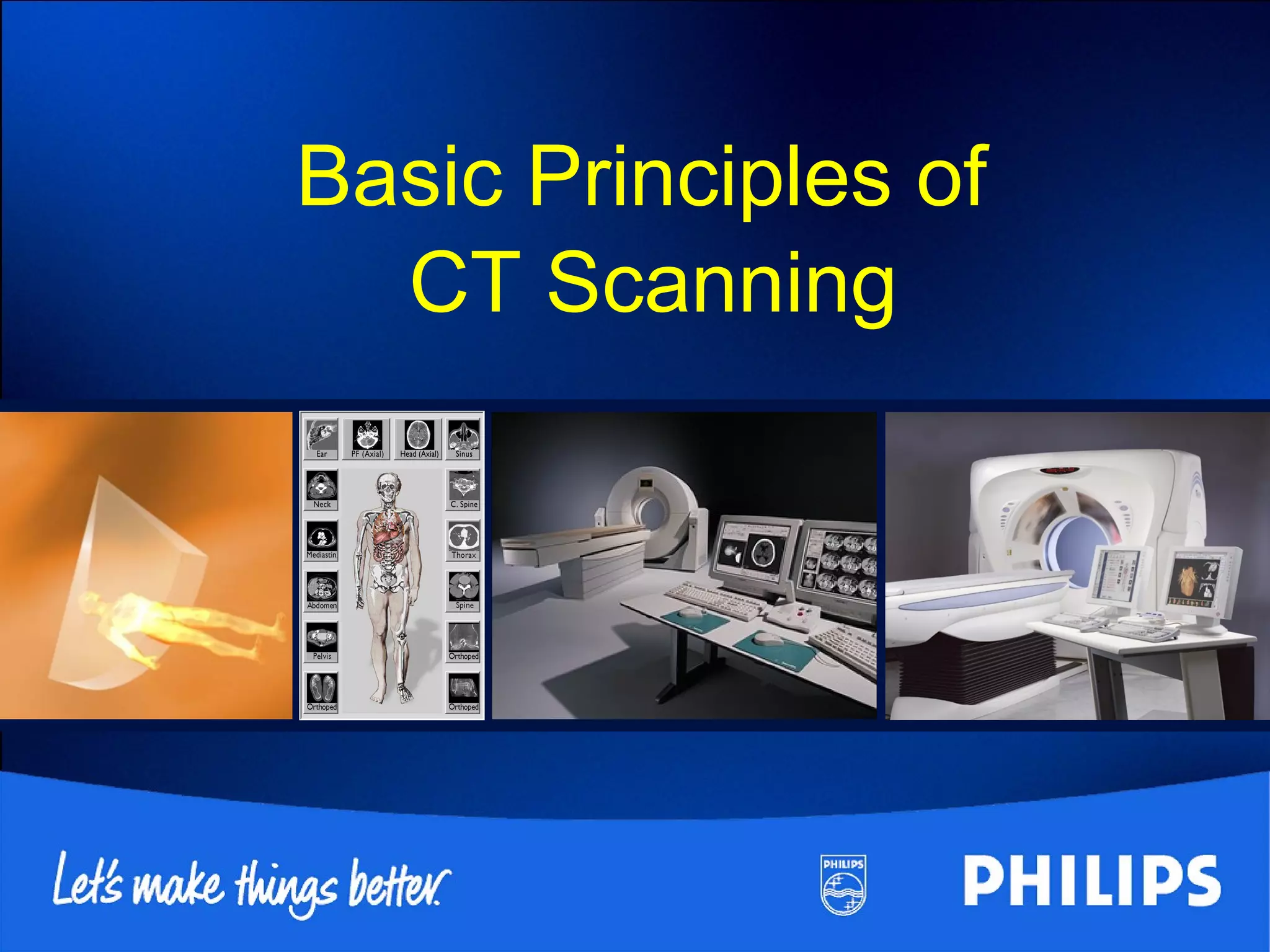
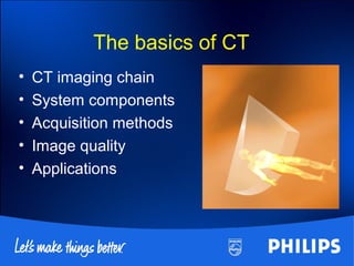
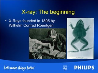
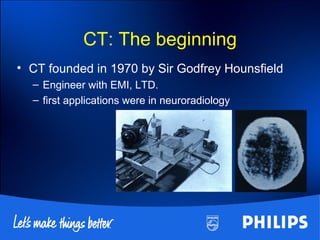
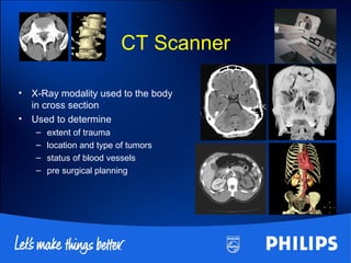
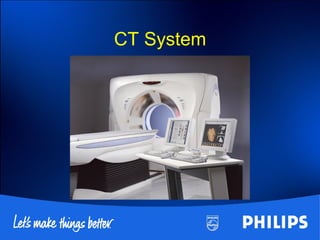
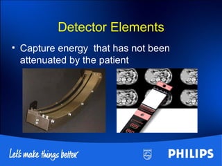
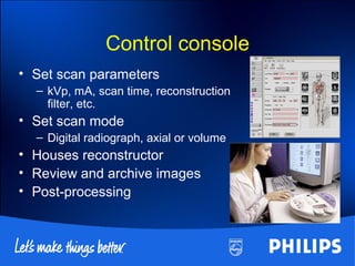
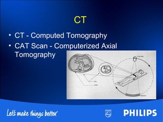
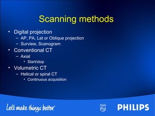
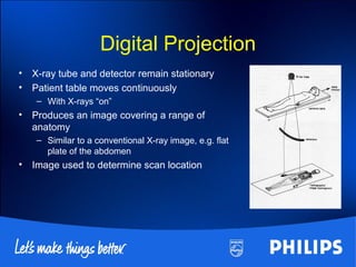
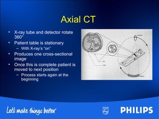
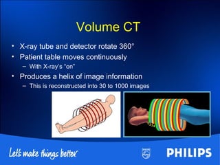
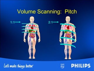

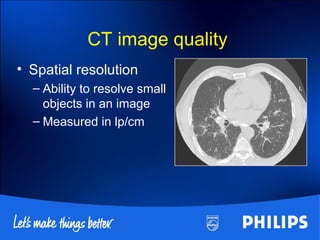
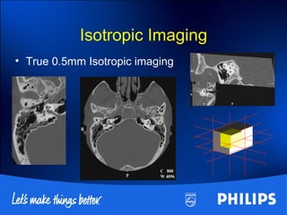
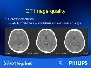
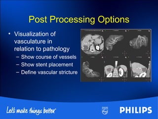

This document discusses the basics of CT scanning, including its history and key components. It describes how CT scanning works, from the x-ray tube emitting radiation that is detected after passing through the body, to the computer using this data to reconstruct cross-sectional images. It outlines the main parts of a CT system, including the gantry, detector, and control console. It also explains different scanning methods and how image quality is determined.