Download as PDF, PPTX

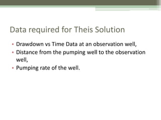
![Several things must be considered before starting a pumping test
1. Literature review or previous report regarding geologic
and hydrogeologic system for the proposed area
2. Pumping test should be carried out within the range of
proposed or designed rate
3. Determine the neraby wells that will be used during the
test if they will be affected.
R0 = 1/2 [(2,25 x T x t /S)]
4. Avoid back flow phenomena with open-end discharge
pipe
5. Measure groundwater levels in both the pumping test
well and nearby wells 24 hours before pumping starts.
Before we start..](https://image.slidesharecdn.com/aquifertestandestimation-160512144215/85/Aquifer-test-and-estimation-5-320.jpg)

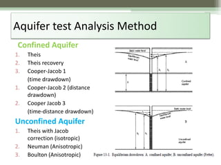
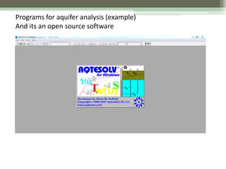


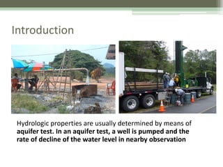
This document discusses methods for conducting and analyzing aquifer tests. It begins by listing objectives of aquifer tests such as measuring hydraulic parameters and determining aquifer properties. It then covers considerations for planning a test and equipment requirements. The document explains concepts such as drawdown, transmissivity, and storativity. It presents equations for analyzing confined and unconfined aquifers, including Theis, Cooper-Jacob, and Neuman models. Finally, it lists some common programs that can be used to analyze aquifer test data.


