Downloaded 175 times
![Hydraulic Conductivity
• Has dimensions of velocity [L/T]
• A combined property of the medium and the fluid
• Ease with which fluid moves through the medium
k = cd2 intrinsic permeability
ρ = density
µ = dynamic viscosity
g = specific weight
Porous medium property
Fluid properties](https://image.slidesharecdn.com/03-darcyslaw-150610082744-lva1-app6891/85/03-darcys-law-12-320.jpg)
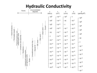
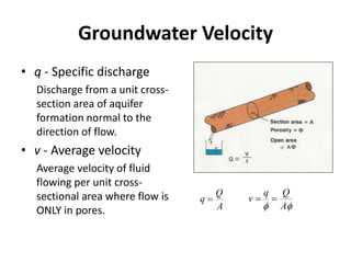
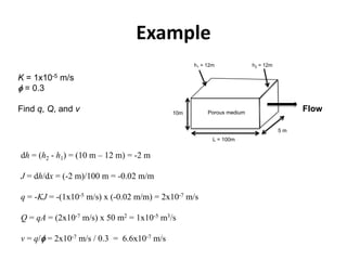
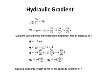

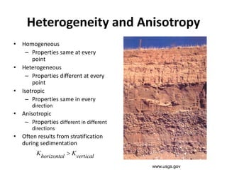


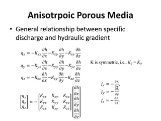
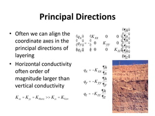
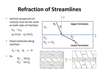

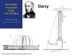
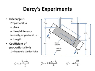
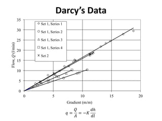
- Darcy's law relates the specific discharge of groundwater to the hydraulic gradient and hydraulic conductivity. It was established based on experiments by Henry Darcy. - Hydraulic conductivity is a property of both the porous medium and fluid that describes the ease of groundwater flow. It can be estimated using the Kozeny-Carman equation or measured in the lab using permeameters. - Groundwater flow is heterogeneous and anisotropic in layered or stratified aquifers. The generalized form of Darcy's law accounts for variable conductivity in different directions. Streamlines refract at interfaces between layers with different conductivities.
![Geotechnical Engineering-I [Lec #23: Soil Permeability]](https://cdn.slidesharecdn.com/ss_thumbnails/23-180924141141-thumbnail.jpg?width=640&height=640&fit=bounds)


