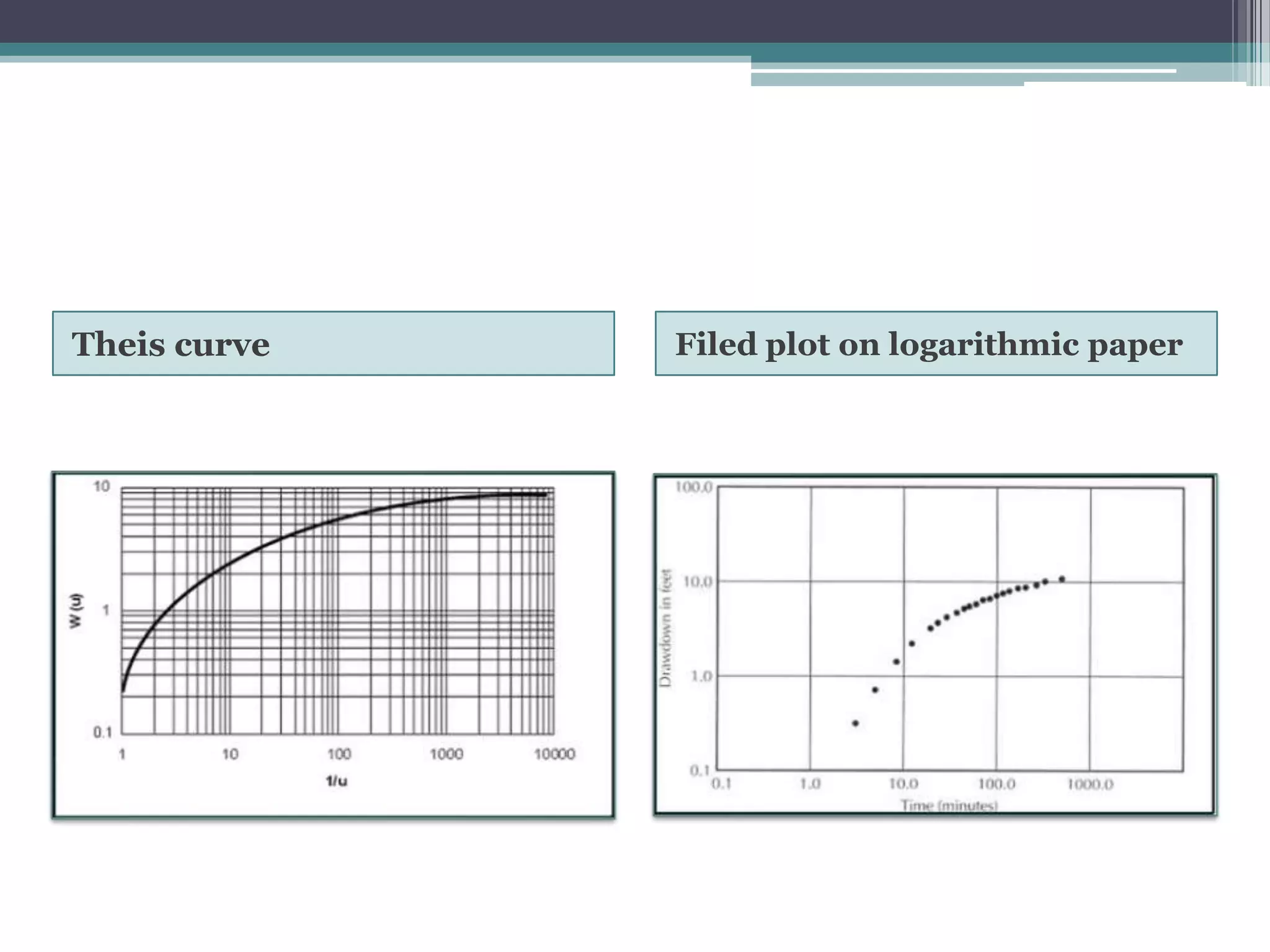
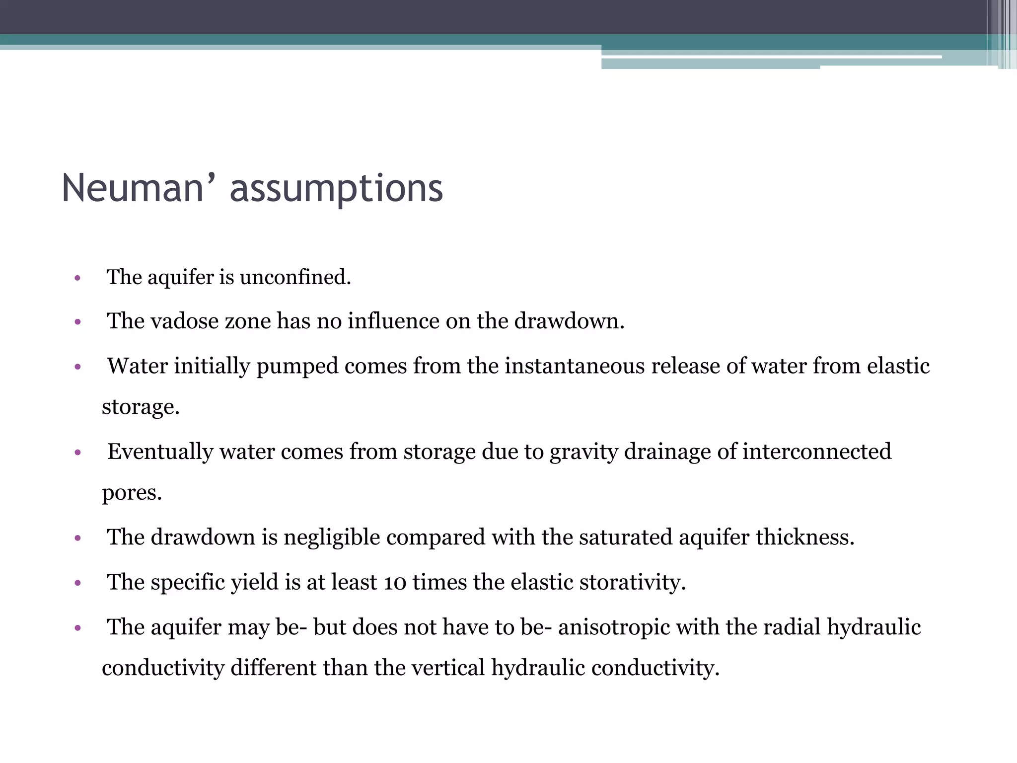
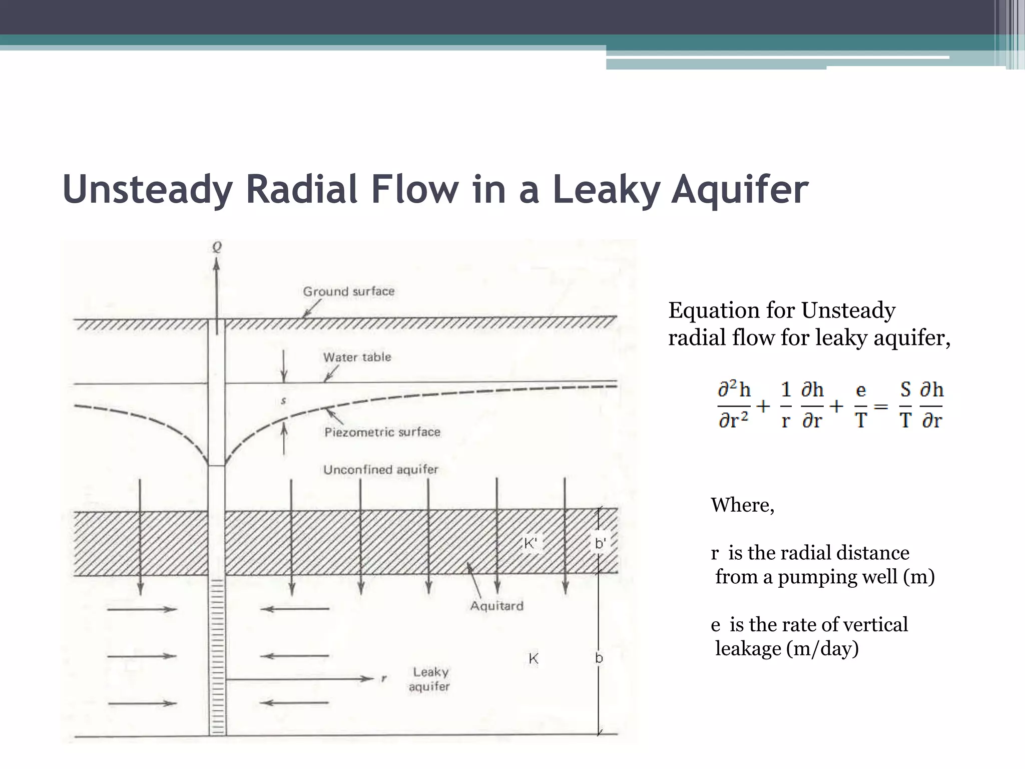
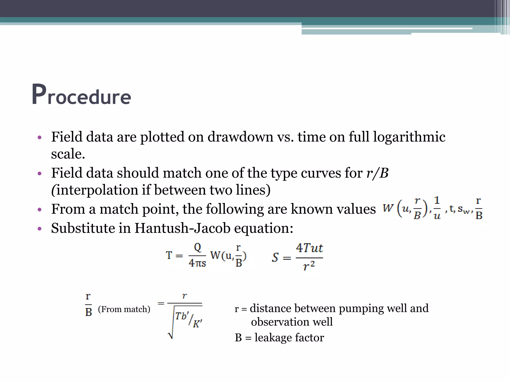
Aquifer and Non Equilibrium
equation for unsteady radial
flow
Presented by: AbhiShek Gupta
Aquifer
• A saturated, permeable, geologic unit that can transmit a
significant amount of groundwater under an ordinary
gradient.
Unsteady flow in confined aquifer
• Assumptions
 The aquifer is confined
 The aquifer has infinite aerial extent
 The aquifer is homogeneous, isotropic and of uniform thickness
 The piezometric surface is horizontal prior to pumping
 The aquifer is pumped at a constant discharge rate
 The well penetrates the full thickness of the aquifer and thus
receives water by horizontal flow
principle of continuity equation
of flow,
Inflow,
Outflow,
• Change in volume,
S (Storage coefficient) is the volume of water released per unit surface area per
unit change in head normal to the surface.
• In this equation, h is head, r is radial distance from the well, S is storage
coefficient, T is transmissivity, and t is the time since the beginning of pumping.
The Theis Method (Curve Matching Method)
• Theis assumed that the well is replaced by a mathematical sink of constant
strength and imposing the boundary conditions h = h0 for t = 0, and h → h0
as r →∞ for t ≥0, the solution,
Where W(u) is the well function and u is given by,
After taking log on both equations,
therefore, a graph of log s against log t should be the same shape as a graph of log
(W(u)) against log (1/u)
constants
Theis curve Filed plot on logarithmic paper
Match of field data plot to Theis Type curve
Cooper-Jacob Method (Time-Drawdown)
This is also based upon the Theis analysis
Base 10
Straight line
If and are drawdown at time
and then,
Transmissivity is calculated by above
equation.
When s=0
(storativity)
Semi –log plot
Cooper-Jacob Method (Distance-Drawdown)
When observation of 3 or more wells are to be made.
transmissivity, per one logarithmic cycle
When s=0,
Therefore,
Unsteady Radial Flow in an Unconfined Aquifer
Equation of flow of water (Neuman’s equation),
where,
h is the saturated thickness of the aquifer (m)
r is radial distance from the pumping well (m)
z is elevation above the base of the aquifer (m)
is specific storage (1/m)
is radial hydraulic conductivity (m/day)
is vertical hydraulic conductivity (m/day)
T is time (day)
Three phases of drawdown
First phase:
• pressure drops
• specific storage as a major
contribution behaves as an
artesian aquifer
•flow is horizontal
• time-drawdown follows
Theis curve S - the elastic
storativity.
Second phase Third phase
• water table declines
• specific yield as a major
contribution
• flow is both horizontal and
vertical
• time-drawdown is a function
of Kv/Kh r, b
• rate of drawdown decreases
• flow is again horizontal
• time-drawdown again follows
Theis curve S - the specific
yield.
Neuman’ assumptions
• The aquifer is unconfined.
• The vadose zone has no influence on the drawdown.
• Water initially pumped comes from the instantaneous release of water from elastic
storage.
• Eventually water comes from storage due to gravity drainage of interconnected
pores.
• The drawdown is negligible compared with the saturated aquifer thickness.
• The specific yield is at least 10 times the elastic storativity.
• The aquifer may be- but does not have to be- anisotropic with the radial hydraulic
conductivity different than the vertical hydraulic conductivity.
Neuman’s solution,
Where,
is the well function of water-table aquifer
For early time,
and
For late time, and
and
Parameters can be
found by Penman
method
Penmen method to find parameters
• Two sets of type curves are used and plotted on log-log paper (Theoretical curve
vs 1/u).
• Superpose the early (t − s) data on Type-A curve.
• The data analysis is done by matching the observed data to the type curve.
• From the match point of Type-A curve, determine the values for
and the value of
• Use the previous equations to determine T and S
• The latest (s − t) data are then superposed on Type-B Curve for the Γ - values of
previously matched Type-A curve, from the match point of Type-B curve, determine
the values for
• By using the previous equations, the T and S can be determined.
.
Type curves for unconfined aquifers
Unsteady Radial Flow in a Leaky Aquifer
Equation for Unsteady
radial flow for leaky aquifer,
Where,
r is the radial distance
from a pumping well (m)
e is the rate of vertical
leakage (m/day)
Hantush-Jacob Method
Assumptions:
• The aquifer is leaky and has an "apparent" infinite extent,
• The aquifer and the confining layer are homogeneous, isotropic, and of uniform
thickness, over the area influenced by pumping,
• The potentiometric surface was horizontal prior to pumping,
• The well is pumped at a constant rate,
• The well is fully penetrating,
• Water removed from storage is discharged instantaneously with decline in head,
• The well diameter is small so that well storage is negligible,
• Leakage through the aquitard layer is vertical.
Hantush and Jacob solution for leaky aquifer,
Where,
where,
is the well function for leaky confined aquifer
B is the leakage factor given as
where,
b' is thickness of the aquitard (m)
K' is hydraulic conductivity of the aquitard (m/day)
Walton Graphical Solution
Log-log plot
Procedure
• Field data are plotted on drawdown vs. time on full logarithmic
scale.
• Field data should match one of the type curves for r/B
(interpolation if between two lines)
• From a match point, the following are known values
• Substitute in Hantush-Jacob equation:
(From match) r = distance between pumping well and
observation well
B = leakage factor
Thank you

Non equilibrium equation for unsteady radial flow

  • 1.
    Aquifer and NonEquilibrium equation for unsteady radial flow Presented by: AbhiShek Gupta
  • 2.
    Aquifer • A saturated,permeable, geologic unit that can transmit a significant amount of groundwater under an ordinary gradient.
  • 3.
    Unsteady flow inconfined aquifer • Assumptions  The aquifer is confined  The aquifer has infinite aerial extent  The aquifer is homogeneous, isotropic and of uniform thickness  The piezometric surface is horizontal prior to pumping  The aquifer is pumped at a constant discharge rate  The well penetrates the full thickness of the aquifer and thus receives water by horizontal flow
  • 4.
    principle of continuityequation of flow, Inflow, Outflow,
  • 5.
    • Change involume, S (Storage coefficient) is the volume of water released per unit surface area per unit change in head normal to the surface. • In this equation, h is head, r is radial distance from the well, S is storage coefficient, T is transmissivity, and t is the time since the beginning of pumping.
  • 6.
    The Theis Method(Curve Matching Method) • Theis assumed that the well is replaced by a mathematical sink of constant strength and imposing the boundary conditions h = h0 for t = 0, and h → h0 as r →∞ for t ≥0, the solution, Where W(u) is the well function and u is given by,
  • 7.
    After taking logon both equations, therefore, a graph of log s against log t should be the same shape as a graph of log (W(u)) against log (1/u) constants
  • 8.
    Theis curve Filedplot on logarithmic paper
  • 9.
    Match of fielddata plot to Theis Type curve
  • 10.
    Cooper-Jacob Method (Time-Drawdown) Thisis also based upon the Theis analysis Base 10 Straight line
  • 11.
    If and aredrawdown at time and then, Transmissivity is calculated by above equation. When s=0 (storativity) Semi –log plot
  • 12.
    Cooper-Jacob Method (Distance-Drawdown) Whenobservation of 3 or more wells are to be made. transmissivity, per one logarithmic cycle When s=0, Therefore,
  • 13.
    Unsteady Radial Flowin an Unconfined Aquifer Equation of flow of water (Neuman’s equation), where, h is the saturated thickness of the aquifer (m) r is radial distance from the pumping well (m) z is elevation above the base of the aquifer (m) is specific storage (1/m) is radial hydraulic conductivity (m/day) is vertical hydraulic conductivity (m/day) T is time (day)
  • 14.
    Three phases ofdrawdown First phase: • pressure drops • specific storage as a major contribution behaves as an artesian aquifer •flow is horizontal • time-drawdown follows Theis curve S - the elastic storativity.
  • 15.
    Second phase Thirdphase • water table declines • specific yield as a major contribution • flow is both horizontal and vertical • time-drawdown is a function of Kv/Kh r, b • rate of drawdown decreases • flow is again horizontal • time-drawdown again follows Theis curve S - the specific yield.
  • 16.
    Neuman’ assumptions • Theaquifer is unconfined. • The vadose zone has no influence on the drawdown. • Water initially pumped comes from the instantaneous release of water from elastic storage. • Eventually water comes from storage due to gravity drainage of interconnected pores. • The drawdown is negligible compared with the saturated aquifer thickness. • The specific yield is at least 10 times the elastic storativity. • The aquifer may be- but does not have to be- anisotropic with the radial hydraulic conductivity different than the vertical hydraulic conductivity.
  • 17.
    Neuman’s solution, Where, is thewell function of water-table aquifer For early time, and For late time, and and Parameters can be found by Penman method
  • 18.
    Penmen method tofind parameters • Two sets of type curves are used and plotted on log-log paper (Theoretical curve vs 1/u). • Superpose the early (t − s) data on Type-A curve. • The data analysis is done by matching the observed data to the type curve. • From the match point of Type-A curve, determine the values for and the value of • Use the previous equations to determine T and S • The latest (s − t) data are then superposed on Type-B Curve for the Γ - values of previously matched Type-A curve, from the match point of Type-B curve, determine the values for • By using the previous equations, the T and S can be determined. .
  • 19.
    Type curves forunconfined aquifers
  • 20.
    Unsteady Radial Flowin a Leaky Aquifer Equation for Unsteady radial flow for leaky aquifer, Where, r is the radial distance from a pumping well (m) e is the rate of vertical leakage (m/day)
  • 21.
    Hantush-Jacob Method Assumptions: • Theaquifer is leaky and has an "apparent" infinite extent, • The aquifer and the confining layer are homogeneous, isotropic, and of uniform thickness, over the area influenced by pumping, • The potentiometric surface was horizontal prior to pumping, • The well is pumped at a constant rate, • The well is fully penetrating, • Water removed from storage is discharged instantaneously with decline in head, • The well diameter is small so that well storage is negligible, • Leakage through the aquitard layer is vertical.
  • 22.
    Hantush and Jacobsolution for leaky aquifer, Where, where, is the well function for leaky confined aquifer B is the leakage factor given as where, b' is thickness of the aquitard (m) K' is hydraulic conductivity of the aquitard (m/day)
  • 23.
  • 24.
    Procedure • Field dataare plotted on drawdown vs. time on full logarithmic scale. • Field data should match one of the type curves for r/B (interpolation if between two lines) • From a match point, the following are known values • Substitute in Hantush-Jacob equation: (From match) r = distance between pumping well and observation well B = leakage factor
  • 25.