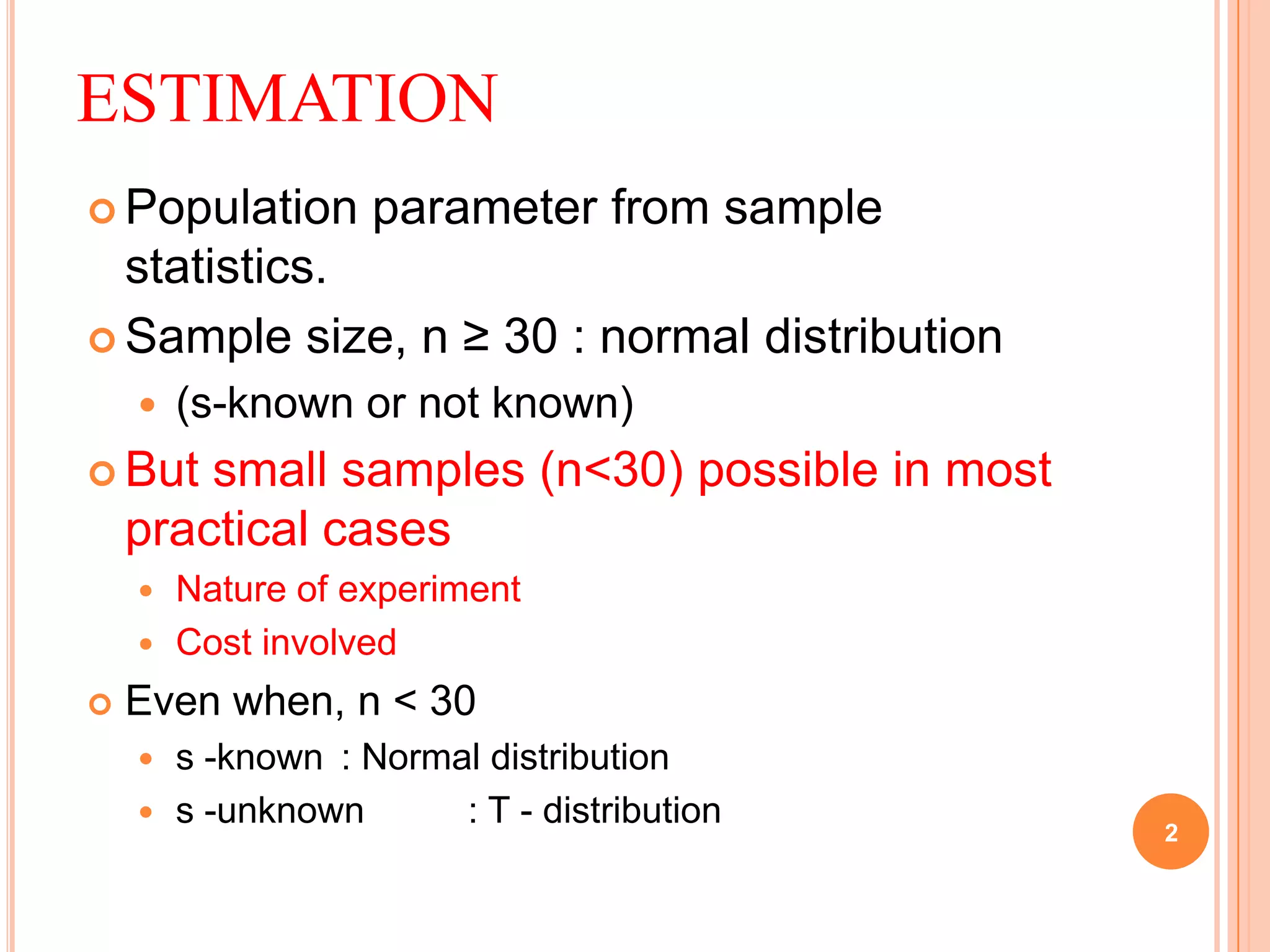
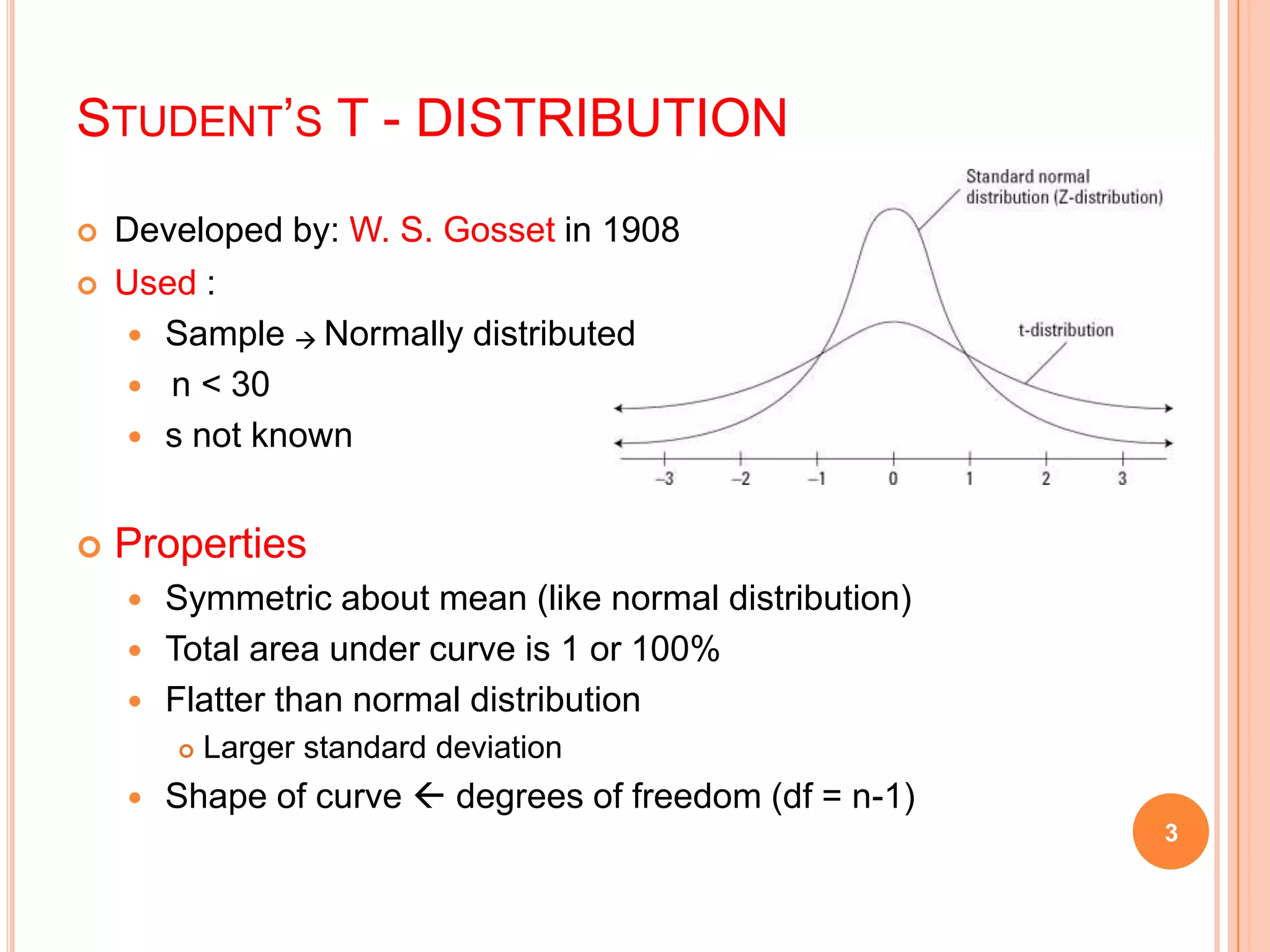
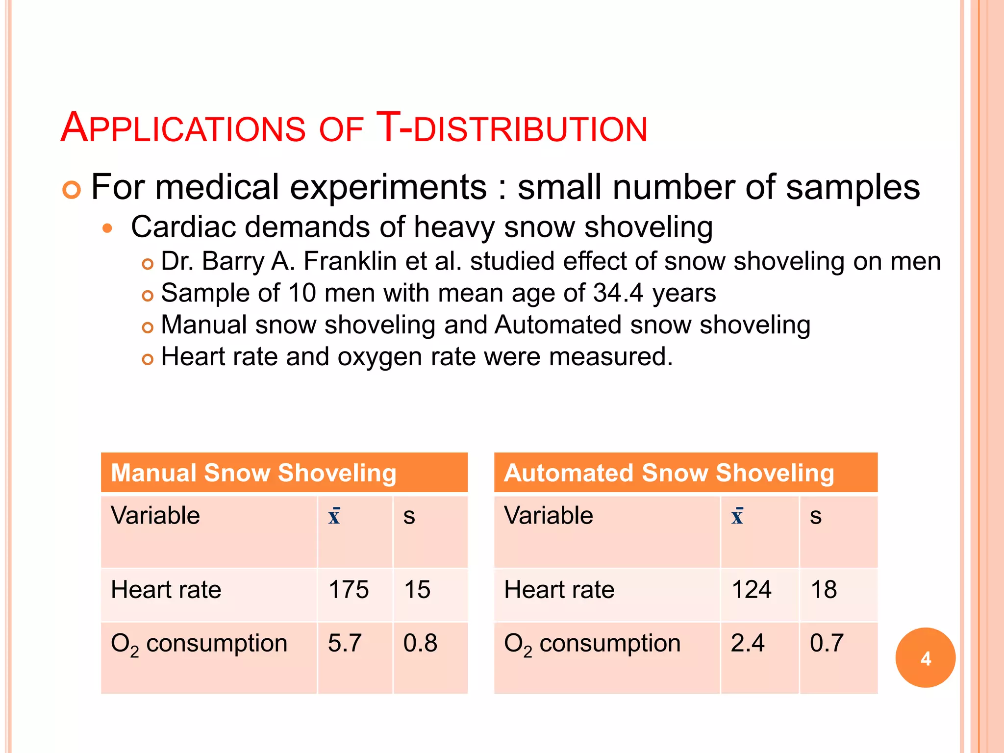
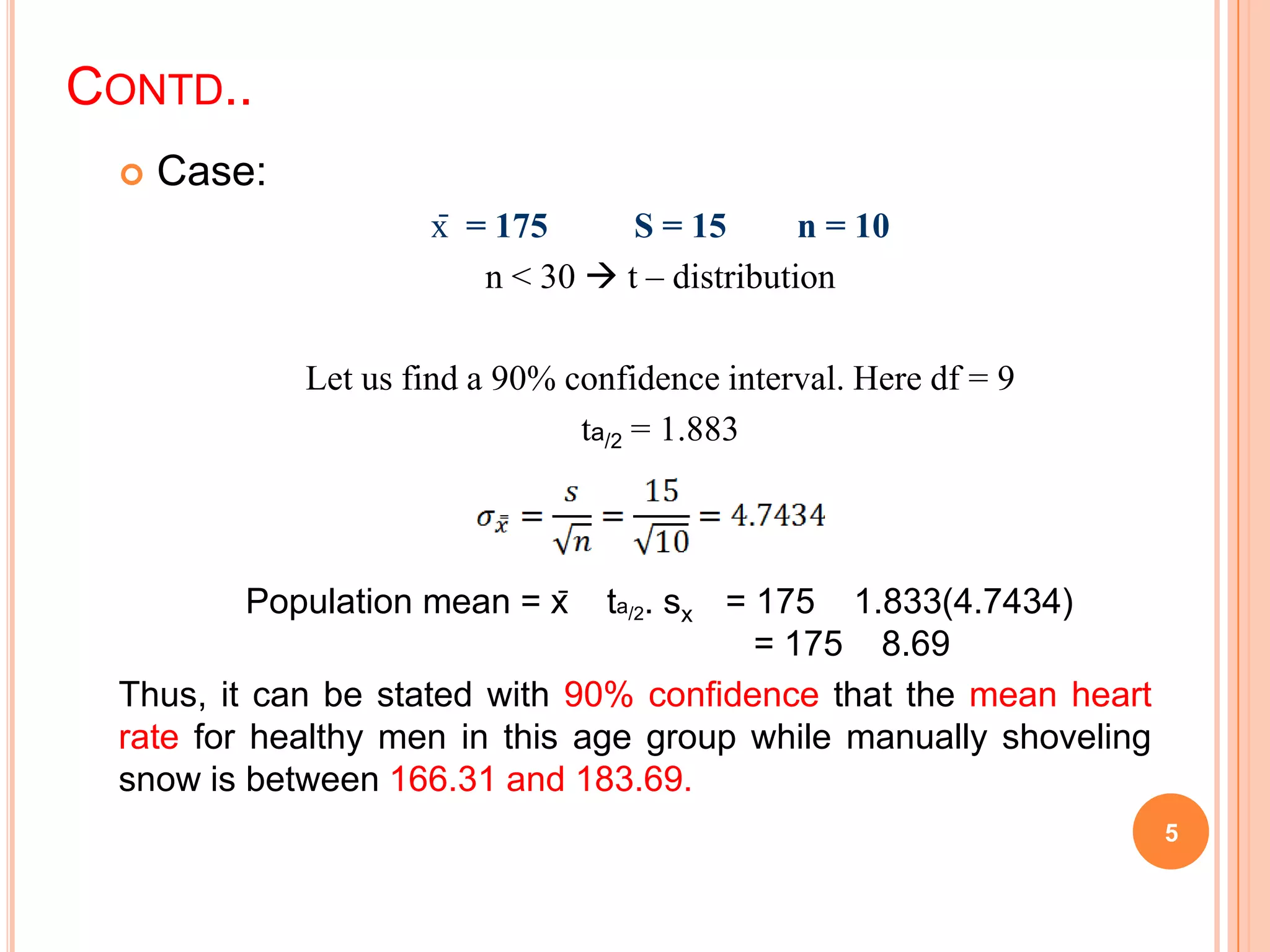
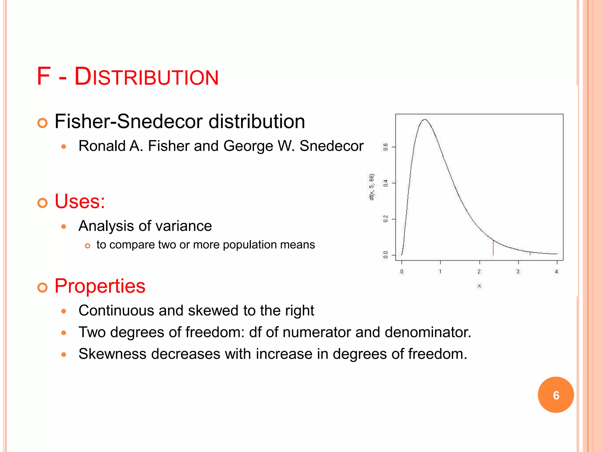
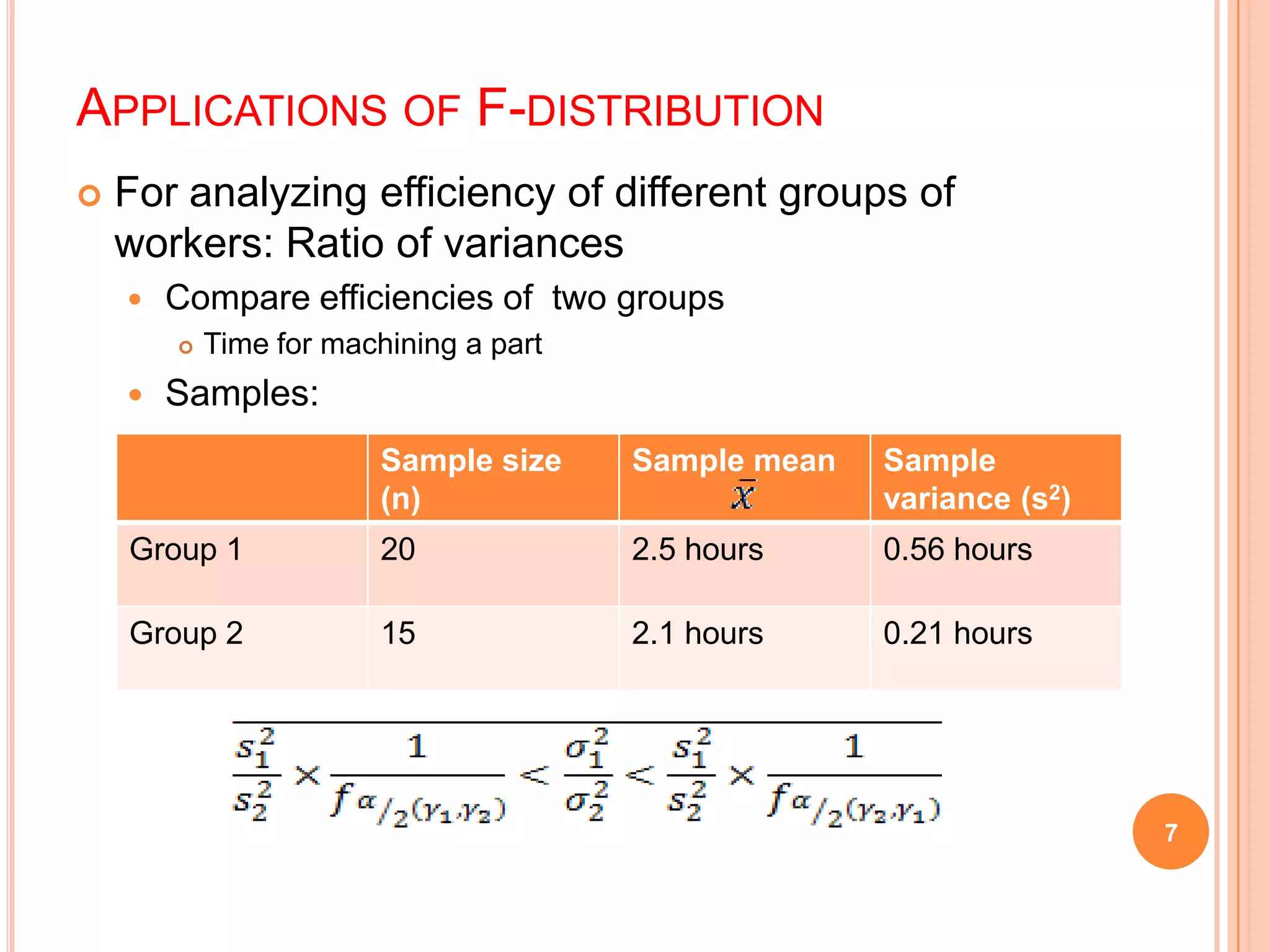
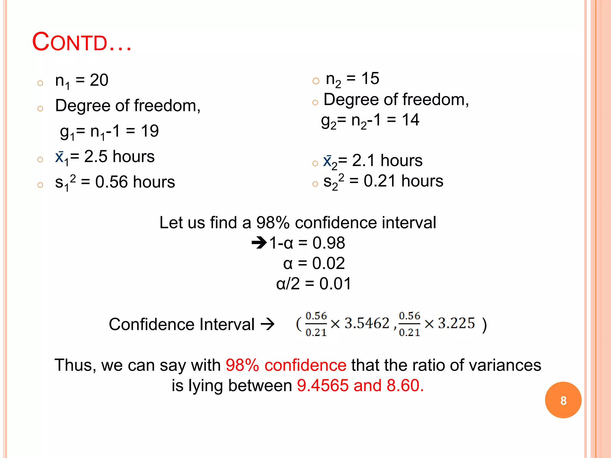
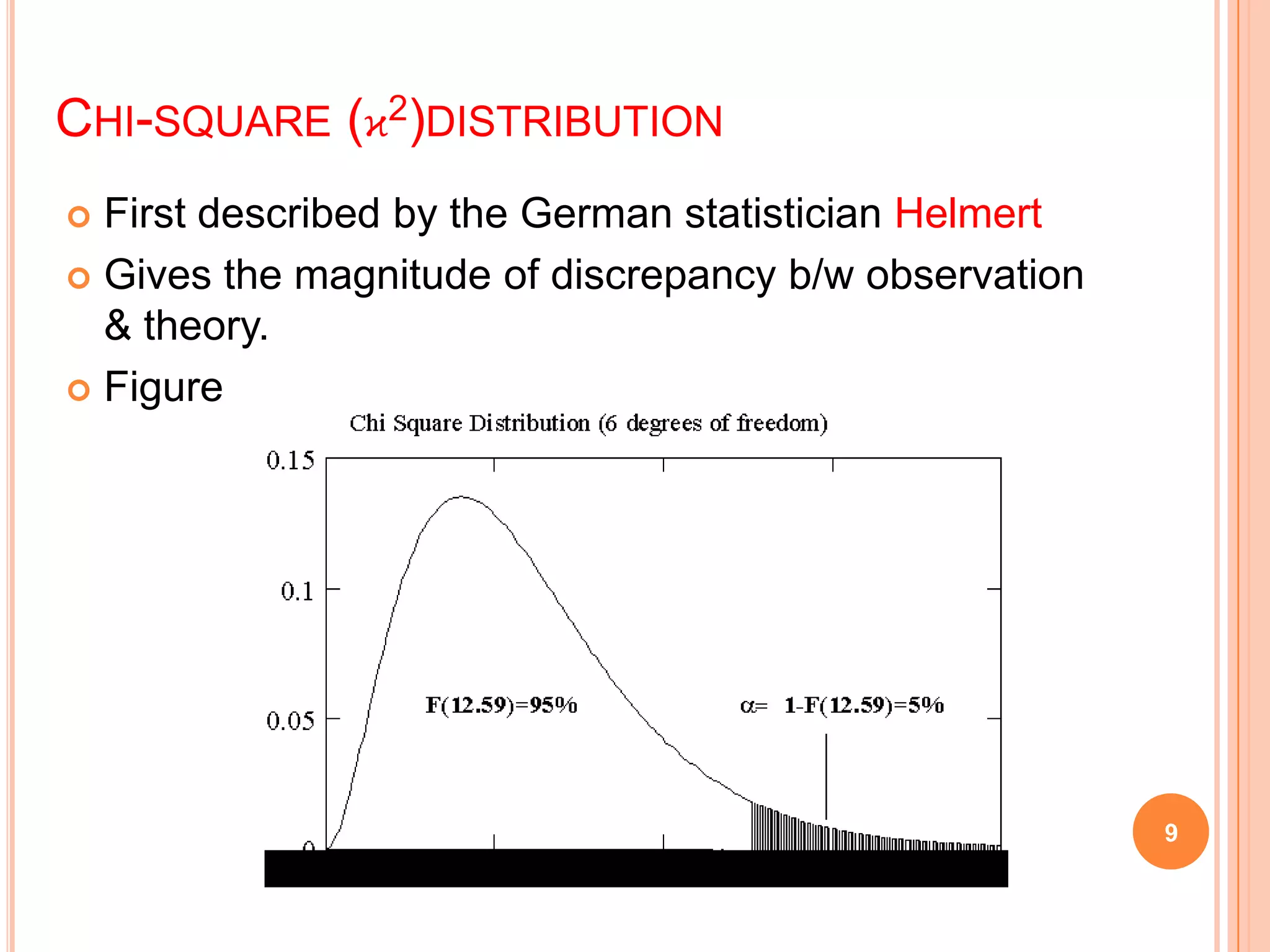
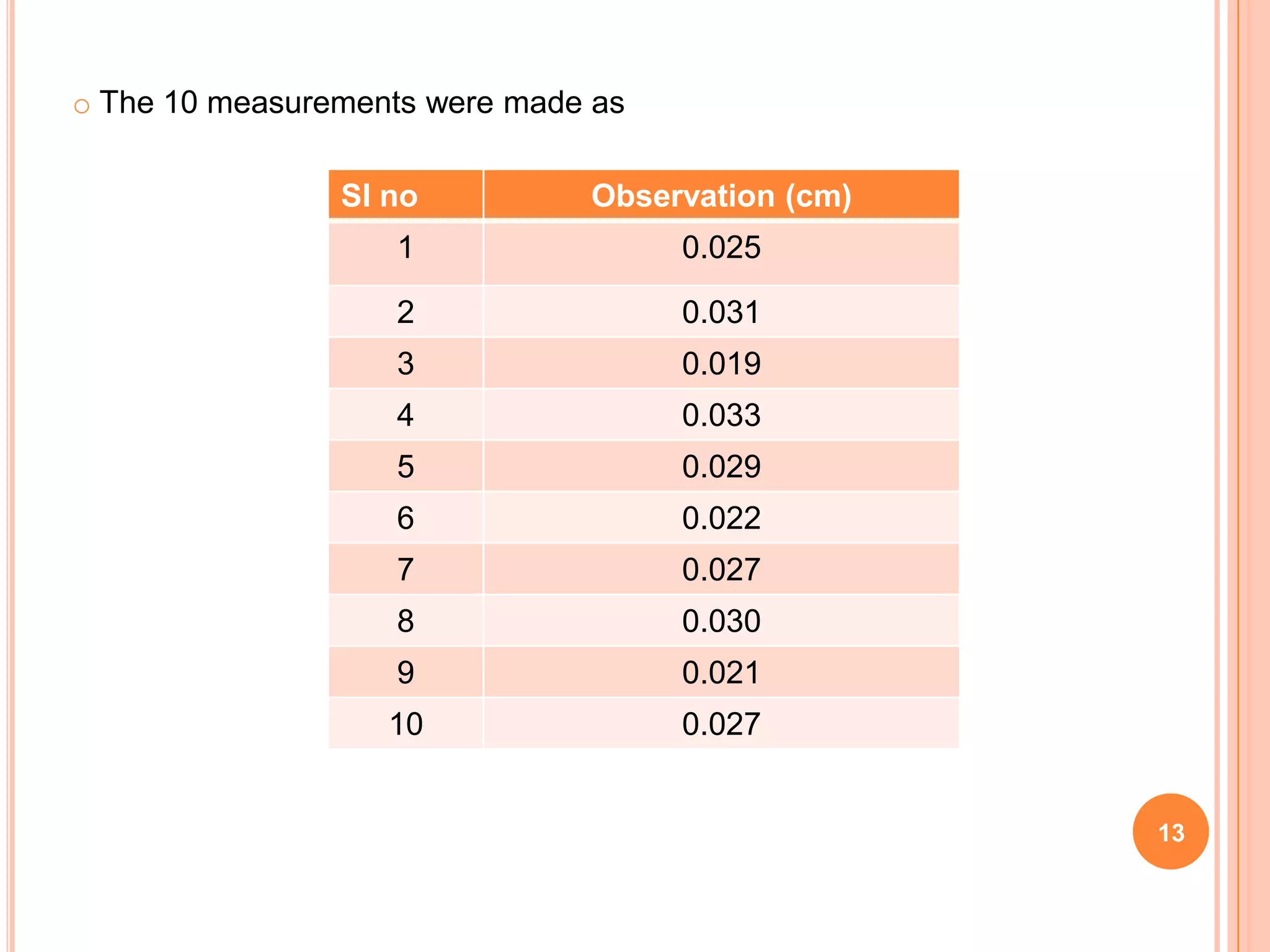
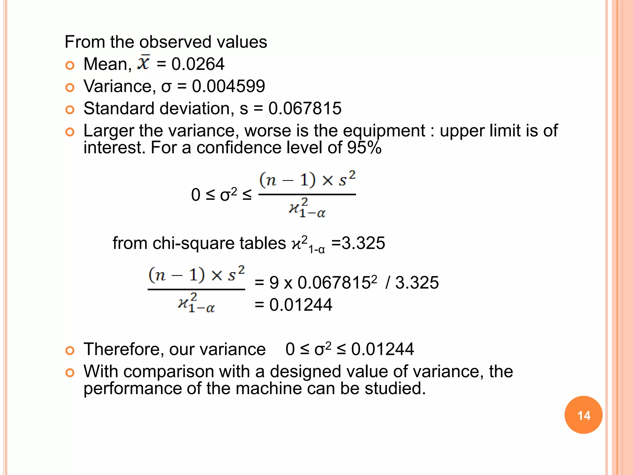
APPLICATIONS OF T, F AND ϰ 2
DISTRIBUTIONS
By
FREDY JAMES J. (13MY03)
JABIN MATHEW BENJAMIN (13MY04)
KARTHICK C. (13MY32)
1
ESTIMATION
 Population parameter from sample
statistics.
 Sample size, n ≥ 30 : normal distribution
 (s-known or not known)
 But small samples (n<30) possible in most
practical cases
 Nature of experiment
 Cost involved
 Even when, n < 30
 s -known : Normal distribution
 s -unknown : T - distribution
2
STUDENT’S T - DISTRIBUTION
 Developed by: W. S. Gosset in 1908
 Used :
 Sample  Normally distributed
 n < 30
 s not known
 Properties
 Symmetric about mean (like normal distribution)
 Total area under curve is 1 or 100%
 Flatter than normal distribution
 Larger standard deviation
 Shape of curve  degrees of freedom (df = n-1)
3
APPLICATIONS OF T-DISTRIBUTION
 For medical experiments : small number of samples
 Cardiac demands of heavy snow shoveling
 Dr. Barry A. Franklin et al. studied effect of snow shoveling on men
 Sample of 10 men with mean age of 34.4 years
 Manual snow shoveling and Automated snow shoveling
 Heart rate and oxygen rate were measured.
4
Manual Snow Shoveling
Variable x̄ s
Heart rate 175 15
O2 consumption 5.7 0.8
Automated Snow Shoveling
Variable x̄ s
Heart rate 124 18
O2 consumption 2.4 0.7
CONTD..
 Case:
x̄ = 175 S = 15 n = 10
n < 30  t – distribution
Let us find a 90% confidence interval. Here df = 9
ta/2 = 1.883
Population mean = x̄ ta/2. sx = 175 1.833(4.7434)
= 175 8.69
Thus, it can be stated with 90% confidence that the mean heart
rate for healthy men in this age group while manually shoveling
snow is between 166.31 and 183.69.
5
F - DISTRIBUTION
 Fisher-Snedecor distribution
 Ronald A. Fisher and George W. Snedecor
 Uses:
 Analysis of variance
 to compare two or more population means
 Properties
 Continuous and skewed to the right
 Two degrees of freedom: df of numerator and denominator.
 Skewness decreases with increase in degrees of freedom.
6
APPLICATIONS OF F-DISTRIBUTION
 For analyzing efficiency of different groups of
workers: Ratio of variances
 Compare efficiencies of two groups
 Time for machining a part
 Samples:
7
Sample size
(n)
Sample mean Sample
variance (s2)
Group 1 20 2.5 hours 0.56 hours
Group 2 15 2.1 hours 0.21 hours
CONTD…
o n1 = 20
o Degree of freedom,
g1= n1-1 = 19
o x̄1= 2.5 hours
o s1
2 = 0.56 hours
8
o n2 = 15
o Degree of freedom,
g2= n2-1 = 14
o x̄2= 2.1 hours
o s2
2 = 0.21 hours
Let us find a 98% confidence interval
1-α = 0.98
α = 0.02
α/2 = 0.01
Confidence Interval  )
Thus, we can say with 98% confidence that the ratio of variances
is lying between 9.4565 and 8.60.
CHI-SQUARE (ϰ2)DISTRIBUTION
 First described by the German statistician Helmert
 Gives the magnitude of discrepancy b/w observation
& theory.
 Figure
9
Properties:
o ϰ2 = (n-1) s2 / σ2
o If ϰ2 =0 then observation & theoretical frequency
completely agree.
o As ϰ2 increases, the discrepancy b/w observation
& theoritical frequency increases.
o Shape depends on degrees of freedom.
o ϰ2 assumes non-negatives only.
o The mean of the distribution is equal to its df.
10
11
o To the practical side....
o Consider the case of a water distribution system used for
irrigation. They should be designed to distribute water uniformly
over an area.
o Failure of uniform application results in non optimum results.
o An equipment that does not supply water uniformly would
probably not be purchased.
12
 A company wishes to check uniformity of a new
model.
 The variances of depth of water measured at
different locations in a field would serve as a
measure of uniformity of water application.
 Say 10 measurements are made, which produced a
variance of 0.004599 or s = 0.067815 cm/hr.
 Here, greater the variance, the poorer is the
equipment.
 So, take an upper limit
o The 10 measurements were made as
Sl no Observation (cm)
1 0.025
2 0.031
3 0.019
4 0.033
5 0.029
6 0.022
7 0.027
8 0.030
9 0.021
10 0.027
13
14
From the observed values
 Mean, = 0.0264
 Variance, σ = 0.004599
 Standard deviation, s = 0.067815
 Larger the variance, worse is the equipment : upper limit is of
interest. For a confidence level of 95%
0 ≤ σ2 ≤
from chi-square tables ϰ2
1-α =3.325
= 9 x 0.0678152 / 3.325
= 0.01244
 Therefore, our variance 0 ≤ σ2 ≤ 0.01244
 With comparison with a designed value of variance, the
performance of the machine can be studied.
THANK YOU
15

Applications of t, f and chi2 distributions

  • 1.
    APPLICATIONS OF T,F AND ϰ 2 DISTRIBUTIONS By FREDY JAMES J. (13MY03) JABIN MATHEW BENJAMIN (13MY04) KARTHICK C. (13MY32) 1
  • 2.
    ESTIMATION  Population parameterfrom sample statistics.  Sample size, n ≥ 30 : normal distribution  (s-known or not known)  But small samples (n<30) possible in most practical cases  Nature of experiment  Cost involved  Even when, n < 30  s -known : Normal distribution  s -unknown : T - distribution 2
  • 3.
    STUDENT’S T -DISTRIBUTION  Developed by: W. S. Gosset in 1908  Used :  Sample  Normally distributed  n < 30  s not known  Properties  Symmetric about mean (like normal distribution)  Total area under curve is 1 or 100%  Flatter than normal distribution  Larger standard deviation  Shape of curve  degrees of freedom (df = n-1) 3
  • 4.
    APPLICATIONS OF T-DISTRIBUTION For medical experiments : small number of samples  Cardiac demands of heavy snow shoveling  Dr. Barry A. Franklin et al. studied effect of snow shoveling on men  Sample of 10 men with mean age of 34.4 years  Manual snow shoveling and Automated snow shoveling  Heart rate and oxygen rate were measured. 4 Manual Snow Shoveling Variable x̄ s Heart rate 175 15 O2 consumption 5.7 0.8 Automated Snow Shoveling Variable x̄ s Heart rate 124 18 O2 consumption 2.4 0.7
  • 5.
    CONTD..  Case: x̄ =175 S = 15 n = 10 n < 30  t – distribution Let us find a 90% confidence interval. Here df = 9 ta/2 = 1.883 Population mean = x̄ ta/2. sx = 175 1.833(4.7434) = 175 8.69 Thus, it can be stated with 90% confidence that the mean heart rate for healthy men in this age group while manually shoveling snow is between 166.31 and 183.69. 5
  • 6.
    F - DISTRIBUTION Fisher-Snedecor distribution  Ronald A. Fisher and George W. Snedecor  Uses:  Analysis of variance  to compare two or more population means  Properties  Continuous and skewed to the right  Two degrees of freedom: df of numerator and denominator.  Skewness decreases with increase in degrees of freedom. 6
  • 7.
    APPLICATIONS OF F-DISTRIBUTION For analyzing efficiency of different groups of workers: Ratio of variances  Compare efficiencies of two groups  Time for machining a part  Samples: 7 Sample size (n) Sample mean Sample variance (s2) Group 1 20 2.5 hours 0.56 hours Group 2 15 2.1 hours 0.21 hours
  • 8.
    CONTD… o n1 =20 o Degree of freedom, g1= n1-1 = 19 o x̄1= 2.5 hours o s1 2 = 0.56 hours 8 o n2 = 15 o Degree of freedom, g2= n2-1 = 14 o x̄2= 2.1 hours o s2 2 = 0.21 hours Let us find a 98% confidence interval 1-α = 0.98 α = 0.02 α/2 = 0.01 Confidence Interval  ) Thus, we can say with 98% confidence that the ratio of variances is lying between 9.4565 and 8.60.
  • 9.
    CHI-SQUARE (ϰ2)DISTRIBUTION  Firstdescribed by the German statistician Helmert  Gives the magnitude of discrepancy b/w observation & theory.  Figure 9
  • 10.
    Properties: o ϰ2 =(n-1) s2 / σ2 o If ϰ2 =0 then observation & theoretical frequency completely agree. o As ϰ2 increases, the discrepancy b/w observation & theoritical frequency increases. o Shape depends on degrees of freedom. o ϰ2 assumes non-negatives only. o The mean of the distribution is equal to its df. 10
  • 11.
    11 o To thepractical side.... o Consider the case of a water distribution system used for irrigation. They should be designed to distribute water uniformly over an area. o Failure of uniform application results in non optimum results. o An equipment that does not supply water uniformly would probably not be purchased.
  • 12.
    12  A companywishes to check uniformity of a new model.  The variances of depth of water measured at different locations in a field would serve as a measure of uniformity of water application.  Say 10 measurements are made, which produced a variance of 0.004599 or s = 0.067815 cm/hr.  Here, greater the variance, the poorer is the equipment.  So, take an upper limit
  • 13.
    o The 10measurements were made as Sl no Observation (cm) 1 0.025 2 0.031 3 0.019 4 0.033 5 0.029 6 0.022 7 0.027 8 0.030 9 0.021 10 0.027 13
  • 14.
    14 From the observedvalues  Mean, = 0.0264  Variance, σ = 0.004599  Standard deviation, s = 0.067815  Larger the variance, worse is the equipment : upper limit is of interest. For a confidence level of 95% 0 ≤ σ2 ≤ from chi-square tables ϰ2 1-α =3.325 = 9 x 0.0678152 / 3.325 = 0.01244  Therefore, our variance 0 ≤ σ2 ≤ 0.01244  With comparison with a designed value of variance, the performance of the machine can be studied.
  • 15.