Download as PDF, PPTX
![Theory & Practice
[Anonymous]
• Theory is when you know something, but it doesn’t work.
• Practice is when something works, but you don’t know why.
• Programmers combine theory and practice: Nothing works
and they don’t know why.
Highway dimension 1](https://image.slidesharecdn.com/20100131highwaydimensiongoldberg-100622124225-phpapp02/85/Andrew-Goldberg-Highway-Dimension-and-Provably-Efficient-Shortest-Path-Algorithms-2-320.jpg)
![Theory & Practice
[Anonymous]
• Theory is when you know something, but it doesn’t work.
• Practice is when something works, but you don’t know why.
• Programmers combine theory and practice: Nothing works
and they don’t know why.
Algorithm Engineering:
Know something ⇒ make it work.
Reverse Engineering:
Something works ⇒ explain why (this talk).
Highway dimension 2](https://image.slidesharecdn.com/20100131highwaydimensiongoldberg-100622124225-phpapp02/85/Andrew-Goldberg-Highway-Dimension-and-Provably-Efficient-Shortest-Path-Algorithms-3-320.jpg)
![Theory & Practice
[Anonymous]
• Theory is when you know something, but it doesn’t work.
• Practice is when something works, but you don’t know why.
• Programmers combine theory and practice: Nothing works
and they don’t know why.
Algorithm Engineering:
Know something ⇒ make it work.
Reverse Engineering:
Something works ⇒ explain why (this talk).
Efficient driving directions: How and why modern routing al-
gorithms work.
Highway dimension 3](https://image.slidesharecdn.com/20100131highwaydimensiongoldberg-100622124225-phpapp02/85/Andrew-Goldberg-Highway-Dimension-and-Provably-Efficient-Shortest-Path-Algorithms-4-320.jpg)
![Motivation
Computing driving directions.
Recent shortest path algorithms (exact):
• Arc flags [Lauther 04, K¨hler et al. 06].
o
• A∗ with landmarks [Goldberg & Harrelson 05].
• Reach [Gutman 04, Goldberg et al. 06].
• Highway [Sanders & Schultes 05] and contraction [Geisberger
08] hierarchies.
• Transit nodes [Bast et al. 06].
• Combinations (pruning and directing algorithms).
Good performance on continent-sized road networks:
Tens of millions of vertices, a few hundred vertices scanned,
under a millisecond on a server, about 0.1 second on a mobile
device. Used in practice.
Highway dimension 4](https://image.slidesharecdn.com/20100131highwaydimensiongoldberg-100622124225-phpapp02/85/Andrew-Goldberg-Highway-Dimension-and-Provably-Efficient-Shortest-Path-Algorithms-5-320.jpg)
![Result Summary
Elegant and practical algorithms, but...
Until now: No analysis for non-trivial network classes and no
understanding of what makes the algorithms work.
Our results:
• We define highway dimension (HD).
• Give provably efficient implementations of several recent al-
gorithms under the small HD assumption.
• Analysis highlights algorithm similarities.
• Give a generative model of small HD networks (road network
formation).
Compare to the small world model [Milgram 67, Kleinberg 99].
Highway dimension 5](https://image.slidesharecdn.com/20100131highwaydimensiongoldberg-100622124225-phpapp02/85/Andrew-Goldberg-Highway-Dimension-and-Provably-Efficient-Shortest-Path-Algorithms-6-320.jpg)
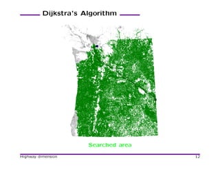
![Dijkstra’s Algorithm
[Dijkstra 1959], [Dantzig 1963].
• At each step scan a labeled vertex with the minimum label.
• Stop when t is selected for scanning.
Work almost linear in the visited subgraph size.
Reverse Algorithm: Run algorithm from t in the graph with all
arcs reversed, stop when s is selected for scanning.
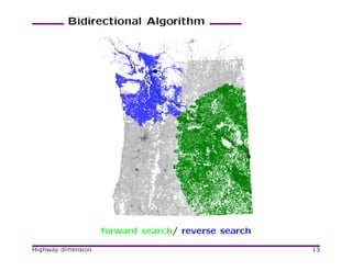
Bidirectional Algorithm
• Run forward Dijkstra from s and backward from t.
• Stopping criteria (careful!).
Highway dimension 10](https://image.slidesharecdn.com/20100131highwaydimensiongoldberg-100622124225-phpapp02/85/Andrew-Goldberg-Highway-Dimension-and-Provably-Efficient-Shortest-Path-Algorithms-11-320.jpg)
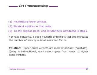
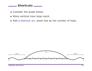
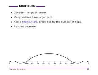
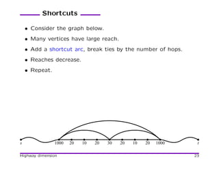
![Contraction Hierarchies
[Geisberget et al. 08] Based on preprocessing that orders vertices
and adds shortcuts. Fast and simple!
Shortcuts:
100
101 110
1 10
11
A shortcut arc can be omitted if redundant (alternative path
exists).
Highway dimension 14](https://image.slidesharecdn.com/20100131highwaydimensiongoldberg-100622124225-phpapp02/85/Andrew-Goldberg-Highway-Dimension-and-Provably-Efficient-Shortest-Path-Algorithms-15-320.jpg)
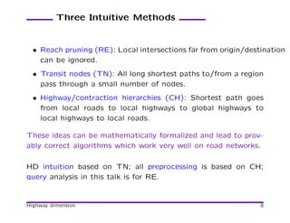
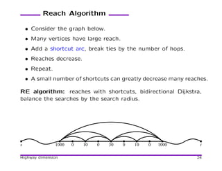
![Reach Definition
[Gutman 04]
• Consider a vertex v that splits a path P into P1 and P2.
rP (v) = min(ℓ(P1), ℓ(P2)).
• r(v) = maxP (rP (v)) over all shortest paths P through v.
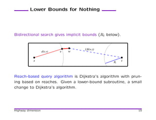
Using reaches to prune Dijkstra:
LB(w,t)
d(s,v) v w
s t
If r(w) < min(d(v) + ℓ(v, w), LB(w, t)) then prune w.
Highway dimension 18](https://image.slidesharecdn.com/20100131highwaydimensiongoldberg-100622124225-phpapp02/85/Andrew-Goldberg-Highway-Dimension-and-Provably-Efficient-Shortest-Path-Algorithms-19-320.jpg)
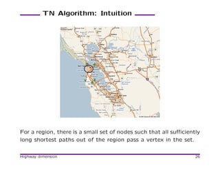
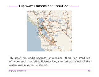
![Transit Node (TN) Algorithm
[Bast et. al 06]
• Divide a map into regions.
• For each region, paths to far away places pass through a
small number of access points.
• The union of all access nodes is the set of transit nodes.
• Preprocessing: find all access points, connect each vertex
to its access nodes, compute all pairs of shortest paths be-
tween transit nodes.
• Query: Look for a “local” shortest path or a shortest path
of the form origin – transit node – transit node – destination.
• Various ways to speed up local queries.
• 10 access nodes per region on the average.
• Leads to the fastest algorithms.
Highway dimension 27](https://image.slidesharecdn.com/20100131highwaydimensiongoldberg-100622124225-phpapp02/85/Andrew-Goldberg-Highway-Dimension-and-Provably-Efficient-Shortest-Path-Algorithms-28-320.jpg)
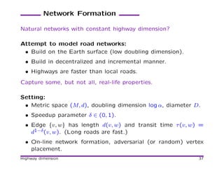
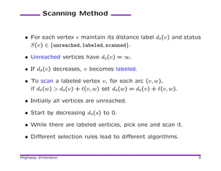
![Network Formation (cont.)
In the spirit of dynamic spanners [Gottlieb & Roditty 08].
• Adversary adds vertices, we connect them.
• Intuition: connect a new village to all nearby villages and to
the closest town.
• Formally: maintain covers Ci for 0 ≤ i ≤ log D.
C0 = V , Ci+1 ⊆ Ci, vertices in Ci are at least 2i apart.
• When adding a new vertex v, add v to C0, . . . , Ci for appro-
priate i. (The first vertex added to all C’s.)
• For 0 ≤ j ≤ i, connect v to Cj ∩ Bv,6·2j .
• If i < log D, connect v to the closest element of Ci+1.
Theorem: The network has highway dimension of αO(1).
Highway dimension 38](https://image.slidesharecdn.com/20100131highwaydimensiongoldberg-100622124225-phpapp02/85/Andrew-Goldberg-Highway-Dimension-and-Provably-Efficient-Shortest-Path-Algorithms-39-320.jpg)


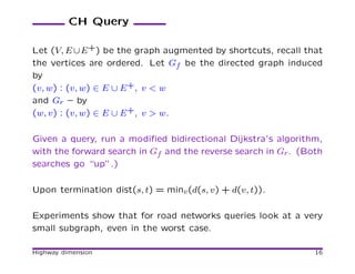
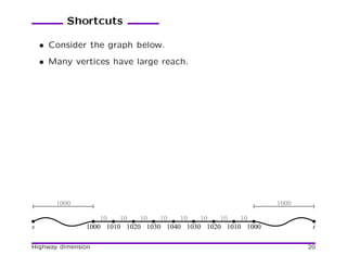
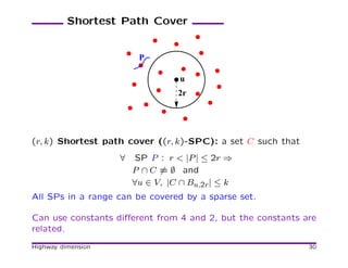
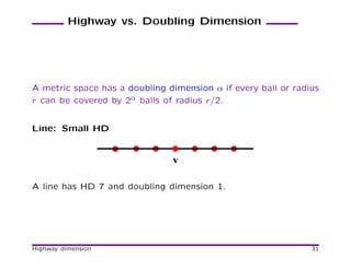
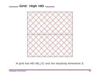
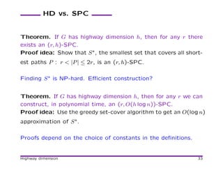
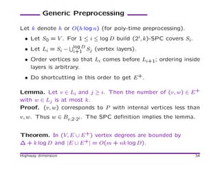
The document describes algorithms for computing shortest paths on road networks and proposes a new concept called highway dimension to explain why these algorithms work efficiently. It defines highway dimension and shows how it relates to other graph metrics. The document also analyzes the query time of reach-based and contraction hierarchy algorithms assuming small highway dimension.