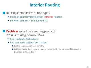
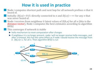
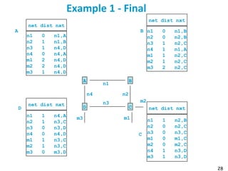
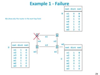
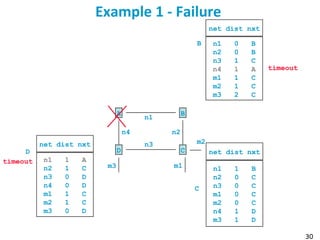
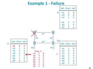
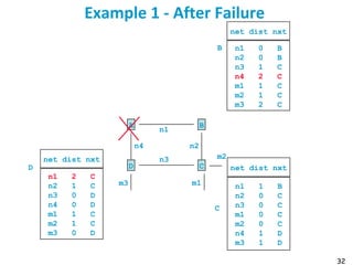
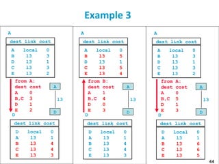
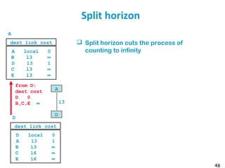
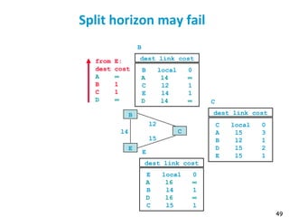
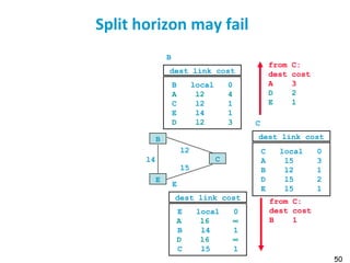
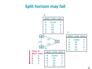
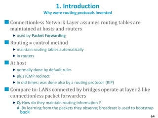
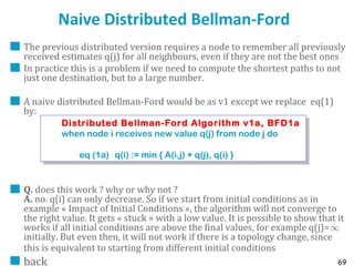
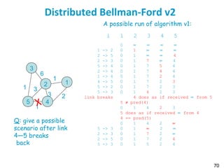
Routing protocols are used to automatically maintain routing tables in routers. Distance vector routing protocols like RIP use the distributed Bellman-Ford algorithm, where each router only knows its local state - the link metrics and estimates of distances to destinations from its neighbors. Using this information, routers periodically exchange distance updates with neighbors and recalculate path costs to determine the optimal next-hop for each destination. While simple and distributed, distance vector protocols are prone to slow convergence and routing loops in certain network conditions.

1. 1
Routing in General
Distance Vector Routing
Jean-Yves Le Boudec
Fall 2009
ÉCOLE POLYTECHNIQUE
FÉDÉRALE DE LAUSANNE

2. 2
Contents
1. Routing in General
2. Distance vector
Bellman-Ford
How it is used in practice
3. Protocols that implement Distance Vector
RIP
RIP v2
IGRP
4. More about routing in general

3. 3
1. Introduction
Why were routing protocols invented
IP assumes routing tables are maintained at hosts and routers used by
Packet Forwarding
Routing = control method
maintain routing tables automatically
in routers
At host routing tables are usually maintained by
default rules
plus ICMP redirect
in old times: was done also by a routing protocol (RIP). Today, a host usually does not
run any routing protocol
Compare to: LANs connected by bridges operate at layer 2 like
connectionless packet forwarders
Q. How do they maintain routing information ?
solution

4. 4
Routing vs Packet Forwarding
Packet Forwarding
for every packet
done in real time
Routing
computation of routing tables or data structures for unicast and multicast
normally only between routers
non-real time: latency up to 2 minutes
uses dedicated protocols (RIP, OSPF, EIGRP (Cisco) for unicast
and DVMRP, M-OSPF, PIM)
ICMP-redirect may alter routing tables, but only in hosts

5. 5
Interior Routing
Routing methods are of two types
Inside an administrative domain = Interior Routing
Between domains = Exterior Routing
Problem solved by a routing protocol
What a routing protocol does
find reachable destinations
find best paths towards destinations
best in the sense of some metric
in this module, best means along shortest path, for some additive metric
(number of hops, delay)

6. 6
Metrics
Distance vector and link state find paths that minimize a metric
Static metric - does not depend on the network state; for example:
number of hops
link capacity and static delay
cost
Dynamic metric- depend on the network state
link load
current delay
see end of section

7. 7
Simple Routing Methods
How routing protocols work
static configuration
for toy networks only
flooding
each packet duplicated on each outgoing link; loops prevented by packet id
or other mechanism ; duplicate packets may be received at destination
simple and robust
no need for routing tables
robust - tolerates link or router failures
optimal in some sense
the first packet has found the shortest path to the destination
costly
many duplicated packets – little useful traffic
used as an ingredient by mobile ad-hoc routing methods (AODV, OLSR)
source routing
source writes route into packet header
router reads next hop from packet header, moves pointer
route discovered by flooding

8. 8
Source Routing
A B 2.2.4
IS
B
IS
IS
IS
A
SA DA RI data
1
2
3
1 2
1 3
1
3
4
3
2
2
4
A B 2.2.4
A B 2.2.4
Q. What are the routes that can be used from A to B ?
solution
A route is described by a sequence of port numbers

9. 9
Route Discovery in Token Rings
B1
A R1
R2
B4
R4
B3
B5
R5
B6
R6
B2
R3
B
One “All Route Broadcast” packet is generated by A. This
creates 5 different packets.
1. A-R1-B1-R2-B2-R3
2. A-R1-B1-R2-B3-R5-B6-R6
3. A-R1-B1-R2-B3-R5-B5-R4
4. A-R1-B4-R4-B5-R5-B3-R2-B2-R3
5. A-R1-B4-R4-B5-R5-B6-R6
2 of them reach B (numbers 2 and 5)
route_1 = R1.B1.R2.B3.R5.B6.R6
route_2 = R1.B4.R4.B5.R5.B6.R6

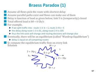
10. 10
In the 1980’s, the token was invented as a competitor to Ethernet. Bridging is in
theory independent of whether we use token ring or ethrnet, however in practice
token ring LANs used source routing bridges instead of spanning tree bridges.
Source routing bridges work as illustrated on the figure:
Bridges and token rings have numbers. Think of a token ring as functionally the same as an
Ethernet collision domain
Assume A has a packet to send to B (here A and B are MAC addresses, but this works equally
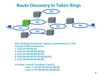
well with IP addresses). A needs to find a description of a route to B. To this end, A floods the
network with an “all-route-broadcast” packet. The packet is generated by A and sent over ring
R1. This packet has a special destination address that means “all-route-broadcast”.
All bridges listen to all rings that they are attached to (this is their job as forwarding devices).
When they see a packet with destination address “all-route-broadcast”, they forward the
packet to all other rings they are attached to, except if the packet has already visited this ring
(the packet contains in its header the list of rings and bridges that it has already visited).
For example, the packet created by A is seen by B1 [resp. B4] who forwards a copy on R2 [resp.
R4]. B2 and B3 see the packet on R2 and forward it to R5 and R3. Etc.
At some point in time, B4 sees a packet on R4 put by B5, which contains as list of visits: “A-R1-
B1-R2-B3-R5-B5-R4” (packet number 3). This packet contains R1 in its list, therefore B4 does not
forward it.
This generates 5 packets in total (numbered 1 to 5 on the figure), 2 of them reach ring R6. When
B sees any of them, it sends an acknowledgement to A. This ack is source routed, along the
reverse route.
A then receives two acks, each of them contains source route information that can be inverted
by A. A now has two routes to B and can choose for example the shortest (in number of hops).
DSR (Dynamic Source Routing) is a protocol for routing in ad-hoc networks that uses
the same mechanism, but with IP addresses instead of MAC addresses.

11. 11
Other Methods
Distance vector (Bellman-Ford)
routers only know their local state
link metric and neighbor estimates
interior routing protocols (RIP, IGRP)
Link state
knowledge of the global state
topology database
global optimization (Shortest Path First - Dijkstra)
interior routing protocols (OSPF, PNNI (ATM))
Path vector
no knowledge of the global state
path: sequence of AS with attributes
global optimization and policy routing
exterior routing protocols (BGP)

12. 12
2. Distance Vector
What it does:
Computes best paths to all destinations
Fully distributed
Using as only information the distances from self to all destinations
How it works
uses distributed Bellman-Ford – see next slides
Note: individual link cost is setup by network management
We first describe the centralized Bellman-Ford algorithm.

13. 13
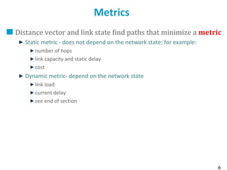
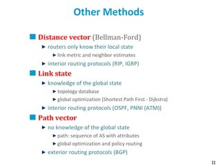
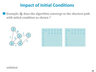
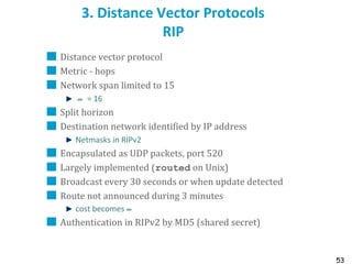
The Centralized Bellman-Ford Algorithm
What: Given a directed graph with links costs A(i,j), computes the best path from i to
j for any couple (i,j).
We assume A(i, j) > 0 and A(i,j) = ∝ when i and j are not connected.
How: Take for example j=1 and let p(i) be the cost of the best path from i to 1.
Define pk
(i) as the cost of the best path from i to 1 in at most k hops. Let p0
(1) = 0, p0
(i) = ∝ for i
≠ 1.
(Bellman Ford, BF1)
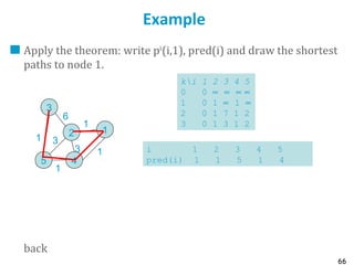
Theorem
1. If the network is fully connected, the algorithm stops at the latest for k=n and then
pk
(i)=p(i) for all i
2. The shortest path from i ≠ 1 to 1 is defined by pred(i) = Argminj≠i [A(i,j) + p(j)].
Idea of Proof: pk
(i) is the distance from i to 1 in at most k hops.
Comment: recursion is equivalent to : pk
(i) = min{ minj≠i,j≠1 [A(i,j) + pk-1
(j)] , A(i,1) }

14. 14
Example
Apply the theorem: write pk
(i), pred(i) and draw the shortest
paths to node 1.
solution
3
2 1
45
6
1
1
1
1 3
3

15. 15
Impact of Initial Conditions
Example: Q. does the algorithm converge to the shortest path
with initial condition as shown ?
solution
3
2 1
45
6
1
1
1
1 3
3
ki 1 2 3 4 5
0 0 0 0 0 0
1
2
3
4
ki 1 2 3 4 5
0 0 6 1 1 0
1
2
3
4

16. 16
Impact of Initial Condition
Theorem
The algorithm converges in a finite number of steps to the correct values
for all initial conditions such that p0
(1)=0 and for every node i that is
connected to 1
If there is no path from i to 1, the algorithm lets pk
(i) converge to 1

17. 17
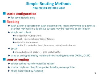
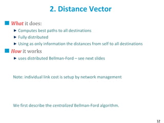
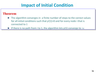
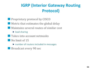
Proof
We do the proof assuming all nodes are connected.
1. Let pk
be the vector pk
[i], i=2,…. Let B be the mapping that transforms an array x[i]i=2…
into the array Bx defined for i ≠ 1 by
Bx[i]=min j≠i,j ≠1[A(i,j) + x(j)]
Let b be the array defined for i ≠ 1 by
b[i]= A(i,1)
The algorithm can be rewritten in vector form as
(1) pk
= B pk-1
∧ b
where ∧ is the pointwise minimum
2. Eq (1) is a min-plus linear equation and the operator B satisfies B(x ∧y)= Bx ∧By.
Thus, Eq(1) can be solved using min-plus algebra into
(2) pk
= Bk
p0
∧ Bk-1
b ∧ … ∧ Bb ∧ b
3. Define the array e for i ≠ 1 by e[i]= ∝. Let p0
=e. Eq (2) becomes
(3) pk
= Bk-1
b ∧ … ∧ Bb ∧ b. Now we have the Bellman Ford algorithm with classical
initial conditions, thus, by Theorem 1:
(4) for k ≥ n-1: Bk-1
b ∧ … ∧ Bb ∧ b = q
where q[i] is the distance from i to 1.
4. We can rewrite Eq(2) for k ≥ n-1 as
(5) pk
= Bk
p0
∧ q
5. Bk
p0
[i] can be written as A[i,i1]+ A[i1,i2]+ …+ A[ik-1,ik]+ p[ik] thus
(6) Bk
p0
[i] ≥ k a, where a is the minimum of all A[i,j]. Thus Bk
p0
[i] tends to ∝ when k
k 0

18. 18
Distributed Bellman Ford
BF1 can be used in a centralized algorithm to compute p(i) i.e. find the shortest path.
However, this is not its main interest, because there is a better algorithm (Dijkstra)
that can be used in a centralized method
But: it can be distributed, as follows.
Theorem: if the time to reliably send a message is bounded by T, the algo converges
to the same result as the centralized version in at most nT time units (if the network
is fully connected)
Distributed Bellman-Ford Algorithm v1, BFD1
every node, say i, maintains an estimate q(i) of the distance p(i) to some
fixed node 1; initial conditions are arbitrary but q(1)=0 at all steps
from time to time, i sends the new value q(i) to all its neighbours
when node i receives a value q(j0) from any neighbour j0, it sets q(j0) to
the received value and updates q(i) by recomputing
eq (1) q(i) := min j neighbour (A(i,j)+q(j))
if eq (1) causes q(i) to be modified, pred(i) is set to a value of j that
achieves the min
Distributed Bellman-Ford Algorithm v1, BFD1
every node, say i, maintains an estimate q(i) of the distance p(i) to some
fixed node 1; initial conditions are arbitrary but q(1)=0 at all steps
from time to time, i sends the new value q(i) to all its neighbours
when node i receives a value q(j0) from any neighbour j0, it sets q(j0) to
the received value and updates q(i) by recomputing
eq (1) q(i) := min j neighbour (A(i,j)+q(j))
if eq (1) causes q(i) to be modified, pred(i) is set to a value of j that
achieves the min

19. 19
Distributed Bellman-Ford v1
3
2 1
45
6
1
2
1
1 3
3
A possible run of algorithm v1. The
table shows the successive values of q(i)
solution
i 1 2 3 4 5
0 ∝ ∝ ∝ ∝
0 1 ∝ ∝ ∝
0 1 ∝ ∝ 4
0 1 7 ∝ 4
0 1 7 5 4
0 1 7 4 4
0 1 7 2 4
0 1 7 2 3
0 1 7 2 3
0 1 4 2 3
1 -> 2
2 -> 5
2 -> 3
5 -> 4
2 -> 4
1 -> 4
4 -> 5
5 -> 2
5 -> 3
link breaks
Q: give a possible
scenario after link
4—5 breaks

20. 20
Naive Distributed Bellman-Ford
The previous distributed version requires a node to remember all previously
received estimates q(j) for all neighbours, even if they are not the best ones
In practice this is a problem if we need to compute the shortest paths to not
just one destination, but to a large number.
A naive distributed Bellman-Ford would be as v1 except we replace eq(1)
by:
Q. does this work ? why or why not ?
solution
Distributed Bellman-Ford Algorithm v1a, BFD1a
when node i receives new value q(j) from node j do
eq (1a) q(i) := min { A(i,j) + q(j), q(i) }
Distributed Bellman-Ford Algorithm v1a, BFD1a
when node i receives new value q(j) from node j do
eq (1a) q(i) := min { A(i,j) + q(j), q(i) }

21. 21
Distributed Bellman-Ford, cont’d
There is an alternative algorithm, that requires only to remember the best
neighbour (pred(i))
Distributed Bellman-Ford Algorithm, version 2 BFD2
every node, say i, maintains an estimate q(i) of the distance p(i) to
some fixed node 1; initial conditions are arbitrary but q(1)=0 at all
steps
from time to time, i sends its value q(i) to all its neighbours
when node i receives a value q(j0) from any neighbour j0, it sets
q(j0) to the received value and updates q(i) by recomputing
eq (2) if j0 == pred(i)
then q(i) := A(i,j0)+q(j0)
else q(i) := min { A(i,j0) + q(j0), q(i) }
if eq (2) causes q(i) to be modified, pred(i) is set to j0
Distributed Bellman-Ford Algorithm, version 2 BFD2
every node, say i, maintains an estimate q(i) of the distance p(i) to
some fixed node 1; initial conditions are arbitrary but q(1)=0 at all
steps
from time to time, i sends its value q(i) to all its neighbours
when node i receives a value q(j0) from any neighbour j0, it sets
q(j0) to the received value and updates q(i) by recomputing
eq (2) if j0 == pred(i)
then q(i) := A(i,j0)+q(j0)
else q(i) := min { A(i,j0) + q(j0), q(i) }
if eq (2) causes q(i) to be modified, pred(i) is set to j0

22. 22
Distributed Bellman-Ford v2
Theorem: If the time to reliably send a message to all neighbours and perform local
computations is bounded by T’, then the algorithm BFD2 converges to the correct
values in at most m (T+T’) time units, where m is the number of steps of convergence
of the centralized algorithm with same initial conditions
Comment: The main difference with version 1 is that eq(2) replaces eq(1). Assume
we use v2, and we start from a condition such that q(i) is indeed equal to the
minimum given by eq (1) (which is what, intuitively, is true most of the time).
When j is not equal to pred(i), both eq(1) and eq(2) have the same effect: the new
value of q(i) is the same in both cases. In contrast, if j == pred(i), then eq (2) sets q(i)
to the new value A(i,j)+q(j), whereas eq(1) sets it to minjneighbour (A(i,j)+q(j)). Eq(2)
provides an upper bound on eq(1), in this case. It turns out that the algorithm still
works, by the same mechanism that makes the algorithm work even when the initial
conditions are arbitrary. Indeed, node i will send its new value to all remaining
neighbours, who will in turn do an update and eventually, node i will receive values
of q(j) that will correct the problem. In other words, if the new value of q(i) is too
high (compared to what would be obtained with eq (1)), this is repaired in one round
of exchanges with the neighbours.

23. 23
Distributed Bellman-Ford v2
3
2 1
45
6
1
2
1
1 3
3
A possible run of algorithm v1:
i 1 2 3 4 5
0 ∝ ∝ ∝ ∝
0 1 ∝ ∝ ∝
0 1 ∝ ∝ 4
0 1 7 ∝ 4
0 1 7 5 4
0 1 7 4 4
0 1 7 2 4
0 1 7 2 3
0 1 7 2 3
0 1 4 2 3
1 -> 2
2 -> 5
2 -> 3
5 -> 4
2 -> 4
1 -> 4
4 -> 5
5 -> 2
5 -> 3
link breaks
solution
Q: give a possible
scenario after link
4—5 breaks

24. 24
How it is used in practice
Node i computes shortest path and next hop for all network prefixes n that it
heard of.
Initially: D(i,n) = 0 if i directly connected to n and D(i,n) = +∞ for any n that
was never heard of.
Node i receives from neighbour k latest values of D(k,n) for all n (this is the
distance vector). Node i computes the best estimates according to algorithm
BFD2
This converges if network is stable
hello mechanism to reset computation after changes
if neighbour k is no longer present, node i will no longer receive hello messages, and
after a timeout, this has the same effect as if node i would receive the message from
k: D(k,n)=1 for all n. Then algorithm BFD2 is run
c(i,m)
c(i,1) D(1,n)
c(i,k) D(k,n)
D(m,n)
i n
1
k
m

25. 25
Example 1
n1
A B
n3
D C
n2n4
net dist nxt
n1 0 n1,A
n4 0 n4,A
net dist nxt
n1 0 n1,B
n2 0 n2,B
net dist nxt
n3 0 n3,D
n4 0 n4,D
m3 0 m3,D
net dist nxt
n2 0 n2,C
n3 0 n3,C
m1 0 m1,C
m2 0 m2,C
A B
CD
m1
m2
m3

26. 26
Example 1
n1
A B
n3
D C
n2n4
net dist nxt
n1 0 n1,A
n4 0 n4,A
net dist nxt
n1 0 n1,B
n2 0 n2,B
n4 1 n1,A
net dist nxt
n3 0 n3,D
n4 0 n4,D
m3 0 m3,D
net dist nxt
n2 0 n2,C
n3 0 n3,C
m1 0 m1,C
m2 0 m2,C
n4 1 n3,D
m3 1 n3,D
from A
n1 0
n4 0
A B
CD
m1
m2
m3
from D
n3 0
n4 0
m3 0

27. 27
Example 1
n1
A B
n3
D C
n2n4
net dist nxt
n1 0 n1,A
n4 0 n4,A
net dist nxt
n3 0 n3,D
n4 0 n4,D
m3 0 m3,D
net dist nxt
n2 0 n2,C
n3 0 n3,C
m1 0 m1,C
m2 0 m2,C
n4 1 n3,D
m3 1 n3,D
A
CD
m1
m2
m3
from C
n2 0
n3 0
m1 0
m2 0
n4 1
m3 1
net dist nxt
n1 0 n1,B
n2 0 n2,B
n3 1 n2,C
n4 1 n1,A
m1 1 n2,C
m2 1 n2,C
m3 2 n2,C
B

28. 28
Example 1 - Final
n1
A B
n3
D C
n2n4
net dist nxt
n1 0 n1,A
n2 1 n1,B
n3 1 n4,D
n4 0 n4,A
m1 2 n4,D
m2 2 n4,D
m3 1 n4,D
net dist nxt
n1 1 n4,A
n2 1 n3,C
n3 0 n3,D
n4 0 n4,D
m1 1 n3,C
m2 1 n3,C
m3 0 m3,D
A
C
D
m1
m2
m3
net dist nxt
n1 1 n2,B
n2 0 n2,C
n3 0 n3,C
m1 0 m1,C
m2 0 m2,C
n4 1 n3,D
m3 1 n3,D
net dist nxt
n1 0 n1,B
n2 0 n2,B
n3 1 n2,C
n4 1 n1,A
m1 1 n2,C
m2 1 n2,C
m3 2 n2,C
B

29. 29
Example 1 - Failure
n1
A B
n3
D C
n2n4
m1
m2
m3
net dist nxt
n1 1 A
n2 1 C
n3 0 D
n4 0 D
m1 1 C
m2 1 C
m3 0 D
D
C
net dist nxt
n1 1 B
n2 0 C
n3 0 C
m1 0 C
m2 0 C
n4 1 D
m3 1 D
net dist nxt
n1 0 B
n2 0 B
n3 1 C
n4 1 A
m1 1 C
m2 1 C
m3 2 C
B
We show only the router in the next hop field

30. 30
Example 1 - Failure
n1
A B
n3
D C
n2n4
m1
m2
m3
timeout
net dist nxt
n1 0 B
n2 0 B
n3 1 C
n4 1 A
m1 1 C
m2 1 C
m3 2 C
B
C
net dist nxt
n1 1 B
n2 0 C
n3 0 C
m1 0 C
m2 0 C
n4 1 D
m3 1 D
net dist nxt
n1 1 A
n2 1 C
n3 0 D
n4 0 D
m1 1 C
m2 1 C
m3 0 D
D
timeout

31. 31
Example 1 - Failure
n1
A B
n3
D C
n2n4
m1
m2
m3
net dist nxt
n1 0 B
n2 0 B
n3 1 C
m1 1 C
m2 1 C
m3 2 C
B
C
net dist nxt
n1 1 B
n2 0 C
n3 0 C
m1 0 C
m2 0 C
n4 1 D
m3 1 D
net dist nxt
n1 2 C
n2 1 C
n3 0 D
n4 0 D
m1 1 C
m2 1 C
m3 0 D
D
From C:
n1 1 B
n2 0 C
n3 0 C
m1 0 C
m2 0 C
n4 1 D
m3 1 D

32. 32
Example 1 - After Failure
n1
A B
n3
D C
n2n4
m1
m2
m3
net dist nxt
n1 0 B
n2 0 B
n3 1 C
n4 2 C
m1 1 C
m2 1 C
m3 2 C
B
C
net dist nxt
n1 1 B
n2 0 C
n3 0 C
m1 0 C
m2 0 C
n4 1 D
m3 1 D
net dist nxt
n1 2 C
n2 1 C
n3 0 D
n4 0 D
m1 1 C
m2 1 C
m3 0 D
D

33. 33
Example 1: conclusions
Example 1 illustrates
how Bellman Ford is mapped to the network concepts
how topology changes are taken into account
most recent announcement replaces previous ones
non refreshed announcements become obsolete
how distance vector carries reachability information

34. 34
Example 2
dest link cost
A local 0
B l1 1
D l3 1
C l1 2
E l1 2
A
l1
A B
l6
D E
l4l3 C
l5
l2
dest link cost
B local 0
A l1 1
C l2 1
E l4 1
D l1 2
B
dest link cost
C local 0
A l2 2
B l2 1
D l2 3
E l2 2
C
dest link cost
D local 0
A l3 1
B l3 2
C l3 3
E l6 1
D
dest link cost
E local 0
A l4 2
B l4 1
D l6 1
C l4 2
E
To simplify, we identify destination with router
Assume algorithm has converged
cost =1
cost =1
cost =1
cost =1
cost =5

35. 35
Example 2
l1
A B
l6
D E
l4l3 C
l5
 we now show only table entries: to C
 link 2 fails
 B updates its table
C l1 2 C l2 ∞
C l3 3 C l4 2
C local 0

36. 36
Example 2: Link failure
 Just before B updates its table, A broadcasts its table with cost 2
to C
 B updates
l1
A B
l6
D E
l4l3 C
l5
C l1 2 C l1 3
C l3 3 C l4 2
from A: C l1 2
C local 0

37. 37
Example 2: Link failure
B sends update to A and E
A and E update
l1
A B
l6
D E
l4l3 C
l5
C l1 4 C l1 3
C l3 3 C l4 4
from B: C l1 3
from B: C l1 3
C local 0

38. 38
Example 2: Link failure
C sends update
it is ignored by E because it it less good
l1
A B
l6
D E
l4l3 C
l5
C l1 4 C l1 3
C l3 3 C l4 4
C local 0
from C: C local 0

39. 39
Example 2: Link failure
A broadcasts its table with cost 4 to C
B updates … we have a loop between A and C
cost is increase by 2 at every iteration
l1
A B
l6
D E
l4l3 C
l5
C l1 4 C l1 5
C l3 3 C l4 4
from A: C l1 4
C local 0

40. 40
Example 2: Link failure
l1
A B
l6
D E
l4l3 C
l5
C l1 6 C l1 7
C l3 7 C l5 5
from C: C local 0
E now accepts announcement from C
C local 0

41. 41
Example 2: Link failure
l1
A B
l6
D E
l4l3 C
l5
C l1 7 C l4 6
C l6 6 C l5 5
E sends announcements to D and B
B and D send announcements to A
the algorithm has converged – stable state
from E: C l5 5
from B: C l4 6
from E: C l5 5
C local 0

42. 42
Conclusions from Example 2
the algorithm converges after modification of the topology, but
the convergence may be very slow
bounce effect
Q: during convergence time, how are routing tables ?
solution

43. 43
Example 3
dest link cost
A local 0
B l3 3
D l3 1
C l3 3
E l3 2
A
A B
D E
l4l3 C
l5
l2
dest link cost
B local 0
A l4 3
C l2 1
E l4 1
D l4 2
B
dest link cost
C local 0
A l5 3
B l2 1
D l5 2
E l5 1
C
dest link cost
D local 0
A l3 1
B l3 ∞
C l6 ∞
E l6 ∞
D
dest link cost
E local 0
A l6 2
B l4 1
D l6 1
C l5 1
E
Assume now all link costs are equal to 1
Links l1 and l6 fail
D detects failure and sets costs to 1

44. 44
Example 3
dest link cost
A local 0
B l3 3
D l3 1
C l3 3
E l3 2
A
A
D
l3
dest link cost
D local 0
A l3 1
B l3 4
C l3 4
E l3 3
D
from A:
dest cost
A 0
B,C 3
D 1
E 2
dest link cost
A local 0
B l3 5
D l3 1
C l3 5
E l3 4
A
A
D
l3
dest link cost
D local 0
A l3 1
B l3 4
C l3 4
E l3 3
D
from B:
dest cost
A 1
B,C 4
D 0
E 3
dest link cost
A local 0
B l3 3
D l3 1
C l3 3
E l3 2
A
A
D
l3
dest link cost
D local 0
A l3 1
B l3 6
C l3 6
E l3 5
D
from A:
dest cost
A 0
B,C 5
D 1
E 3

45. 45
Conclusion from Example 3
The costs to C, B, E grow unbounded “Count to Infinity”
the true costs are infinite
Convergence to a stable state if we set
∞ = large number
e.g. RIP: ∞ = 16
“Split Horizon”
a heuristic to prevent this
if A routes packets to X via B, it does not announce this route to B

46. 46
Example 3: with Split Horizon
dest link cost
A local 0
B l3 3
D l3 1
C l3 3
E l3 2
A
A B
D E
l4l3 C
l5
l2
dest link cost
B local 0
A l4 3
C l2 1
E l4 1
D l4 2
B
dest link cost
C local 0
A l5 3
B l2 1
D l5 2
E l5 1
C
dest link cost
D local 0
A l3 1
B l3 ∞
C l6 ∞
E l6 ∞
D
dest link cost
E local 0
A l6 2
B l4 1
D l6 1
C l5 1
E

47. 47
Example 3: with Split Horizon
dest link cost
A local 0
B l3 3
D l3 1
C l3 3
E l3 2
A
A
D
l3
dest link cost
D local 0
A l3 1
B l3 ∞
C l6 ∞
E l6 ∞
D
from A:
dest cost
A 0

48. 48
Split horizon
dest link cost
A local 0
B l3 ∞
D l3 1
C l3 ∞
E l3 ∞
A
A
D
l3
dest link cost
D local 0
A l3 1
B l3 ∞
C l6 ∞
E l6 ∞
D
from D:
dest cost
D 0
B,C,E ∞
 Split horizon cuts the process of
counting to infinity

49. 49
Split horizon may fail
B
E
l4 C
l5
l2
dest link cost
B local 0
A l4 ∞
C l2 1
E l4 1
D l4 ∞
B
dest link cost
C local 0
A l5 3
B l2 1
D l5 2
E l5 1
C
dest link cost
E local 0
A l6 ∞
B l4 1
D l6 ∞
C l5 1
E
from E:
dest cost
A ∞
B 1
C 1
D ∞

50. 50
Split horizon may fail
B
E
l4 C
l5
l2
dest link cost
B local 0
A l2 4
C l2 1
E l4 1
D l2 3
B
dest link cost
C local 0
A l5 3
B l2 1
D l5 2
E l5 1
C
dest link cost
E local 0
A l6 ∞
B l4 1
D l6 ∞
C l5 1
E
from C:
dest cost
A 3
D 2
E 1
from C:
dest cost
B 1

51. 51
Split horizon may fail
B
E
l4 C
l5
l2
dest link cost
B local 0
A l2 4
C l2 1
E l4 1
D l2 3
B
dest link cost
C local 0
A l5 3
B l2 1
D l5 2
E l5 1
C
dest link cost
E local 0
A l4 5
B l4 1
D l4 4
C l5 1
E
from B:
dest cost
A 4
B 0
C 1
D 3

52. 52
Conclusion: Distance Vector
convergence to stable state may be slow after changes
count to infinity must be prevented by setting a maximum
distance

53. 53
3. Distance Vector Protocols
RIP
Distance vector protocol
Metric - hops
Network span limited to 15
∞ = 16
Split horizon
Destination network identified by IP address
Netmasks in RIPv2
Encapsulated as UDP packets, port 520
Largely implemented (routed on Unix)
Broadcast every 30 seconds or when update detected
Route not announced during 3 minutes
cost becomes ∞
Authentication in RIPv2 by MD5 (shared secret)

54. 54
IGRP (Interior Gateway Routing
Protocol)
Proprietary protocol by CISCO
Metric that estimates the global delay
Maintains several routes of similar cost
load sharing
Takes into account netmasks
No limit of 15
number of routers included in messages
Broadcast every 90 sec

55. 55
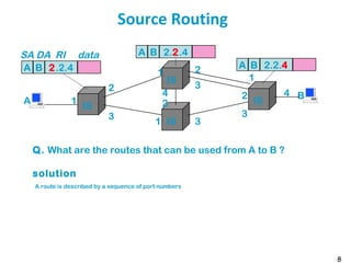
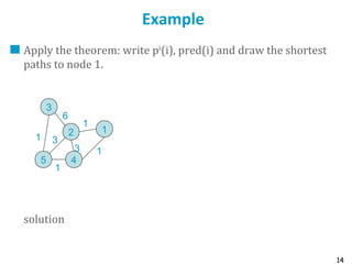
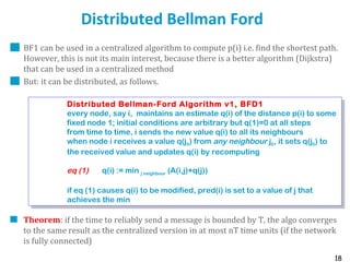
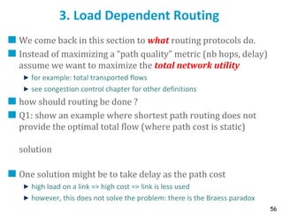
Metric example
Metric
Trans = 10000000/Bandwidth (time to send 10 Kb)
delay = (sum of Delay)/10
m = [K1*Trans + (K2*Trans )/(256-load) + K3*delay]
default: K1=1, K2=0, K3=1, K4=0, K5=0
if K5 ≠ 0, m = m * [K5/(Reliability + K4)]
Bandwidth in Kb/s, Delay in µs
At Venus: Route for 172.17/16: Metric = 10000000/784 +
(20000+1000)/10 = 14855
At Saturn: Route for 12./8: Metric = 10000000/224 + (20000 +
1000)/10 = 46742

56. 56
3. Load Dependent Routing
We come back in this section to what routing protocols do.
Instead of maximizing a “path quality” metric (nb hops, delay)
assume we want to maximize the total network utility
for example: total transported flows
see congestion control chapter for other definitions
how should routing be done ?
Q1: show an example where shortest path routing does not
provide the optimal total flow (where path cost is static)
solution
One solution might be to take delay as the path cost
high load on a link => high cost => link is less used
however, this does not solve the problem: there is the Braess paradox

57. 57
Braess Paradox (1)
Assume all flows pick the route with shortest delay
Assume parallel paths exist and flows can make use of them
Delay is function of load as given below; link 5 is (temporarily) closed
Total offered load is b0 = 6 Gb/s
For example,
if we split traffic into : route 1-3: b = 1, route 2-4 b = 5
the delay along route 1-3 is 61, along route 2-4 is 105
thus the link costs will change and routing decisions will change also
Eventually, there will be an equilibrium (called “Wardrop Equilibrium”)
delay is equal on all competing routes
Q: compute the equilibrium traffic flow on every link
Solution

58. 58
Braess Paradox (2)
Q: same question when we open link 5 with delay function:
Solution

59. 59
Braess Paradox
With shortest delay routing, adding a new link may decrease
overall throughput
Thus shortest delay routing is not either a global optimum

60. 60
Optimal Routing
One can change the objective of routing: instead of computing
shortest paths,one could solve a global optimization problem:
minimize total delay subject to flow constraints
this is a well posed optimization problem
the optimal solution depends on all flows
but it can be implemented in a distributed algorithm similar to TCP
congestion control ; see [BertsekasGallager92]
Q. Can you imagine a way to use classical routing (like distance
vector, which finds shortest paths) and still find the optimum
network utility ?
solution

61. 61
Conclusion
Distance vector is smart
Fully distributed, little information stored
Largely deployed (Unix BSD routed)
Simplicity
But: slow convergence
Not suited for large and complex networks
Link State protocols should be used instead

62. 62
Review Questions
Explain the following terms:
distance vector
bounce effect
count to infinity
split horizon
Bellman Ford
RIP, IGMP
source routing
Explain why shortest path routing is not necessarily a globally
optimum
What is the Braess paradox ?

63. 63
Solutions

64. 64
1. Introduction
Why were routing protocols invented
Connectionless Network Layer assumes routing tables are
maintained at hosts and routers
used by Packet Forwarding
Routing = control method
maintain routing tables automatically
in routers
At host
normally done by default rules
plus ICMP redirect
in old times: was done also by a routing protocol (RIP)
Compare to: LANs connected by bridges operate at layer 2 like
connectionless packet forwarders
Q. How do they maintain routing information ?
A. By learning from the packets they observe; broadcast is used to bootstrap
back

65. 65
Source Routing
A B 2.2.4
IS
B
IS
IS
IS
A
SA DA RI data
1
2
3
1 2
1 3
1
3
4
3
2
2
4
A B 2.2.4
A B 2.2.4
Q. What are the routes that can be used from A to B ?
A. A 2 2 4
A 2 3 4
A 2 4 3 4
A 3 3 4
A 3 2 2 4
A 3 2 3 4
back
A route is described by a sequence of port numbers

66. 66
Example
Apply the theorem: write pk
(i,1), pred(i) and draw the shortest
paths to node 1.
back
3
2 1
45
6
1
1
1
1 3
3 i 1 2 3 4 5
pred(i) 1 1 5 1 4
ki 1 2 3 4 5
0 0 ∝ ∝ ∝ ∝
1 0 1 ∝ 1 ∝
2 0 1 7 1 2
3 0 1 3 1 2

67. 67
Impact of Initial Conditions
Example: Q. does the algorithm
converge to the shortest path with
initial condition as shown ? A. yes
3
2 1
45
6
1
1
1
1 3
3
ki 1 2 3 4 5
0 0 0 0 0 0
1 0 1 1 1 1
2 0 1 2 1 2
3 0 1 3 1 2
4 0 1 3 1 2
ki 1 2 3 4 5
0 0 6 1 1 0
1 0 1 1 1 2
2 0 1 3 1 2

68. 68
Distributed Bellman-Ford v1
3
2 1
45
6
1
2
1
1 3
3
A possible run of algorithm v1:
i 1 2 3 4 5
0 ∝ ∝ ∝ ∝
0 1 ∝ ∝ ∝
0 1 ∝ ∝ 4
0 1 7 ∝ 4
0 1 7 5 4
0 1 7 4 4
0 1 7 2 4
0 1 7 2 3
0 1 7 2 3
0 1 4 2 3
4 does as if received ∝ from 5
5 does as if received ∝ from 4
and continue computations from
there
0 1 4 2 4
0 1 5 2 4
1 -> 2
2 -> 5
2 -> 3
5 -> 4
2 -> 4
1 -> 4
4 -> 5
5 -> 2
5 -> 3
link breaks
5 -> 3
back
Q: give a possible
scenario after link
4—5 breaks

69. 69
Naive Distributed Bellman-Ford
The previous distributed version requires a node to remember all previously
received estimates q(j) for all neighbours, even if they are not the best ones
In practice this is a problem if we need to compute the shortest paths to not
just one destination, but to a large number.
A naive distributed Bellman-Ford would be as v1 except we replace eq(1)
by:
Q. does this work ? why or why not ?
A. no. q(i) can only decrease. So if we start from initial conditions as in
example « Impact of Initial Conditions », the algorithm will not converge to
the right value. It gets « stuck » with a low value. It is possible to show that it
works if all initial conditions are above the final values, for example q(j)=1
initially. But even then, it will not work if there is a topology change, since
this is equivalent to starting from different initial conditions
back
Distributed Bellman-Ford Algorithm v1a, BFD1a
when node i receives new value q(j) from node j do
eq (1a) q(i) := min { A(i,j) + q(j), q(i) }
Distributed Bellman-Ford Algorithm v1a, BFD1a
when node i receives new value q(j) from node j do
eq (1a) q(i) := min { A(i,j) + q(j), q(i) }

70. 70
Distributed Bellman-Ford v2
3
2 1
45
6
1
2
1
1 3
3
A possible run of algorithm v1:
i 1 2 3 4 5
0 ∝ ∝ ∝ ∝
0 1 ∝ ∝ ∝
0 1 ∝ ∝ 4
0 1 7 ∝ 4
0 1 7 5 4
0 1 7 4 4
0 1 7 2 4
0 1 7 2 3
0 1 7 2 3
0 1 4 2 3
4 does as if received ∝ from 5
5 ≠ pred(4)
0 1 4 2 3
5 does as if received ∝ from 4
4 == pred(5)
0 1 4 2 ∝
0 1 ∝ 2 ∝
0 1 7 2 ∝
0 1 7 2 4
0 1 5 2 4
1 -> 2
2 -> 5
2 -> 3
5 -> 4
2 -> 4
1 -> 4
4 -> 5
5 -> 2
5 -> 3
link breaks
5 -> 3
2 -> 3
2 -> 5
5 -> 3back
Q: give a possible
scenario after link
4—5 breaks

71. 71
Conclusions from Example 2
Q: during convergence time, how are routing tables ?
A:
they are incorrect
there are loops – packets are discarded (TTL expires)
back

72. 72
3. Load Dependent Routing
Q. show an example where shortest path routing does not provide the optimal
total flow (where path cost is static)
A. assume all data flow goes from B to E: Static shortest path routing will pick
the direct link BE only instead of distributing the load also on some of the
longer links (BADE and BCE)
back
l1
A B
l6
D E
l4l3 C
l5
l2
E
cost =1
cost =1
cost =1
cost =1
cost =5

73. 73
Braess Paradox (1)
A. there are two paths
1: links 1, 3; 2: links 2,4
let bi be the traffic on path I
Delay equations:
50+ 11b1 = 50 + 11b2
Total flow
b1 + b2 = b0
equilibrium is for b1 = b2 = 3
delay is 83
back

74. 74
Braess Paradox (2)
Q: same question when we open link 5 with delay function:
A: there are three paths
1: links 1, 3;
2: links 2,4;
3: links 1, 5, 4
delay equations
50 + 11b1 + 10b3 = 50 + 11b2 + 10b3 = 10 + 10b1 + 10 b2 + 21 b3
total flow
b1 + b2 + b3 = b0
We find b1= b2 = b3 = 2 Gb/s
The total delay on all paths is the same, equal to 92 : larger than before!

75. 75
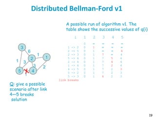
Optimal Routing
One can change the objective of routing: instead of computing
shortest paths,one could solve a global optimization problem:
minimize total delay subject to flow constraints
this is a well posed optimization problem
the optimal solution depends on all flows
but it can be implemented in a distributed algorithm similar to TCP
congestion control ; see [BertsekasGallager92]
Q. Can you imagine a way to use classical routing (like distance
vector, which finds shortest paths) and still find the optimum
network utility ?
A.
Let a centralized network management procedure update the link costs
(used by distance vector routing).
given link costs ci and traffic matrix compute total throughput or average
delay ( a hard optimization problem, solved with heuristics)
every few minutes, update the link costs in all routers – let the routing
algorithm compute new paths
back