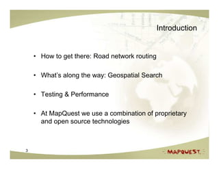
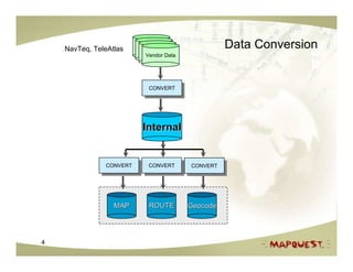
Routing and IP in Advance Computer Network,Vikram Snehi
CPOSC Presentation 20091017
1. How to Get There and What’s Along the Way:
Driving Directions and Geospatial Search
CPOSC, Oct 17 2009
Eric Beyeler
Senior Software Engineer
ebeyeler@mapquest.com
1
2. Introduction
Geospatial information is becoming
integral to our daily lives
2
3. Introduction
• How to get there: Road network routing
• What’s along the way: Geospatial Search
• Testing & Performance
• At MapQuest we use a combination of proprietary
and open source technologies
3
4. NavTeq, TeleAtlas Data Conversion
Vendor Data
CONVERT
CONVERT
Internal
CONVERT
CONVERT CONVERT
CONVERT CONVERT
CONVERT
MAP ROUTE Geocode
4
5. How to Get There
• Geocode address to find lat, lng position of origin,
destination, and any intermediate locations
• Search map data to find closest routable road
links
• Determine best path A -> B
• Create narrative / driving directions
• Extract route shape and road IDs
• Format route results to return to client
5
6. Overview of Shortest Path Methods
Online illustration of Dijkstra’s Algorithm
http://docs.linux.cz/programming/algorithms/Algorithms-
Morris/dijkstra.html
Some interesting sources:
http://theory.stanford.edu/~amitp/GameProgramming/
6
7. Shortest Path Algorithms
• Network is defined as a directed graph G = (N, A)
– Set of nodes (N)
• Nodes occur at intersections or ends of roads
– Set of arcs (A) or links
• Link represents a road section from one node to another node
– Weight (distance, time, other cost metric) of a link
connecting nodes Directed from one node to another
• Shortest path problem
– Given a network, find the shortest distance or lowest cost
from a set of nodes to another set of nodes
7
8. Shortest Path Algorithm Comparison
Adjacency List
D Done Set
D O
O
πr 2
2
r
Area ≅ πr 2
Area ≅ 2 π =
2 2
Single Tree Dijkstra Two Tree Dijkstra
Spreads out uniformly from origin. At each iteration it Dual ended search where one search emanates from
adds the node in the adjacency list with least cost to the the origin and the other from the destination. Each
done set and evaluates all links from that node. Nodes at search spreads out uniformly and acts similarly to the
the end of these links are added to the adjacency if not single tree Dijkstra search. At each iteration the node
already in the list. If the node is in the adjacency list and with least cost (from either the origin or destination
the new path yields a lower cost, the adjacency list is tree) is evaluated. The search ends when a node is in
updated with new cost and predecessor information. the done set of both the origin and destination tree.
Shortest path is found when the destination node is added Since the search is ordered by least cost we know that
to the done set. the shortest path is through the common node.
16
9. Shortest Path Algorithm Comparison
B
A
O D
O D
C
A* Weighted A*
Spreads out from origin but uses a heuristic of Same idea as A*, except weights are applied
predicted cost to the destination. Nodes in the to the cost to the node and to the predicted
adjacency list are sorted by the addition of cost cost to the destination. Higher weights to the
from the origin to the node plus a prediction of heuristic narrow the search but may exclude a
cost to the destination. In the diagram above, less direct path over higher speed roads. W =
assume nodes A,B,and C all have equal cost from 0 yields Dijkstra and W=1 yields a Best First
the origin. Node B will be selected first since it is Search.
closest to the destination. The heuristic tends to
guide the search towards the destination.
f(v) = g(v) + h(v) f(v) = (1-W) * g(v) + W * h(v)
17
10. Intersection / Turn Costs
• Improves route quality
– Reduce number of left turns
– Reduce maneuvers
Previous link
• Simplified directions L1
– Solve some problem routes
• Local lanes on I-270
– Identify and avoid gates, private roads,
T1 = total Next Link
unpaved roads, etc. accumulated time L2
• Apply time penalty to enter from origin
– Allow more realistic use of road speed for
shortest path determination
• General method
– Apply time at intersections T2 = T1 + intersection time from L1
to L2 + time to traverse L1
– Shortest path algorithm considers time at
intersection plus time to traverse link
(distance/speed)
19
11. Route Improvements in Downtown Areas
New York City: 42nd St near 12th Ave. to 52nd St near 18th Ave.
Without Turn Costing: 5 turns (2 left) With Turn Costing: 2 turns (1 left)
Without turn costing: shortest path method tends to follow shorter distance (diagonal) path
More turns, more complex route narrative.
20
12. Favor Roads with Fewer Intersections
Frederick, MD to Washington DC
Without Turn Costing With Turn Costing
Uses I-270 Local Lanes. Slightly shorter Route uses regular I-270 Lanes. Less
distance, but not preferred. Adds complexity. complex narrative.
Addition of intersection costs – routes favor paths with fewer intersections.
21
13. Urban Avoidance / Density Weighting
• Slightly favor rural areas vs. urban areas
– Apply weight factor to speed based on density of links
Avoid I-95 near NYC Help avoid highways through city
centers in favor of bypasses
23
14. Narrative Generation
The goal is to accurately identify what information
is needed for a driver while detecting and
eliminating extraneous information
25
15. Narrative Generation Flow
Receive link information for a route
Compute stops along the way
Combine links to create maneuvers
Merge maneuvers to collapse narrative
Generate driving directions from maneuvers
26
16. Succinct Driving Direction Example
BEFORE
5: Take the I-95 N/I-95 S exit, exit number 11A/11B, towards BALTIMORE/WASHINGTON.
6: Keep RIGHT at the fork in the ramp.
7: Keep LEFT at the fork in the ramp.
8: Merge onto I-95 S.
AFTER
5: Merge onto I-95 S via EXIT 11B toward WASHINGTON.
27
18. Testing and Quality Analysis
What determines a good route?
– Time
– Distance
– Number of maneuvers
– Types of turns
– Road class
– Urban Area
– Detailed data
32
19. Automated Testing
• Route quality tests executed in the Fitnesse framework
– Web interface on top of Fit
• http://fitnesse.org/
• Fitnesse tests scheduled and archived through
CruiseControl
– http://cruisecontrol.sourceforge.net/
• Selenium is used for front-end web page testing
– http://seleniumhq.org/
33
21. Performance
Motivation for 64 Bit MapWare
• We wanted to lessen the amount of time spent trying to fit data
structures into 4GB (32bit address space). This allows us to
load more data sets into 1 server and not spend time working
around the 4GB single process address space limit.
• Better developer throughput and process management are the
first tangible benefits of this project. The real benefits come in
the future since now that we are on a 64bit platform we are
poised for growth.
• Fully take advantage of new hardware advances
35
22. Routing Performance Testing and Optimization
IntelXeon5150@2.66GHz, 64bit RHEL 5, 8 GB, 4 processors
US 8K route set; numbers in routes calculated per second
MW 32 bit MapWare 64 bit MapWare
threads
4 127/sec; 32/s/proc 178/sec; 44/s/proc
• These tests were a best-case scenario run, 16 GB machines
would be needed for real-world duplication of results
• Processors were running at approx 75-80% utilization during
these tests
• Also ran on a 16 GB machine with 64 bit MapWare;
throughput for 4 threads: 195/sec
• Apples to apples comparison:
64 bit MapWare has ~40% more throughput for routing
37
23. Geospatial Searching
• Lucene text search engine
– http://lucene.apache.org/
• SOLR management layer
– http://lucene.apache.org/solr/
– Web API / caching / replication features
– Runs under Tomcat http://tomcat.apache.org/
• Spatial grid / indexing within Lucene
– Geohash - http://en.wikipedia.org/wiki/Geohash
– Lucene implementation
http://sourceforge.net/projects/locallucene/
39
25. Lucene Document Indexing
Based on an “inverted index”
For every term, list all documents that contain that term.
Pizza Hut
10 139
234 234
568 987
987
41
26. Lucene Document Searching
Create a “term vector” based on documents that match
all criteria
Pizza Hut
10 139 “Pizza Hut”
234 234
568 987
987
42
27. Lucene
Lucene and small documents…
Not a match made in heaven.
Lucene is optimized for indexing and searching large
documents. Document term frequency comes into
play. Which is a problem when the typical
document is 3-4 words.
Lucene is configurable enough that there are ways to
tune it for this kind of dataset.
43
29. Searching on the Spatial Grid
Based on “Geohash” concept
The world is divided into
quadrants based on Lat/Lng
Each quadrant is subdivided into
quadrants, etc.
Every quadrant on every level
gets an ID. A spatial ID is
defined by all the level IDs
needed to identify a “box” at a
particular granularity.
45
32. “That all seems like a lot of
work…
I wish there was a free
Web Service I could use
to do this all for me!”
48
33. Platform Web Services
• Free Web Services for Routing, Mapping,
Geocoding
• Search and traffic on the way!
• www.mapquestapi.com
• http://platform.beta.mapquest.com/
• Easily embed maps and routes in your web page
using only HTML and JavaScript
49