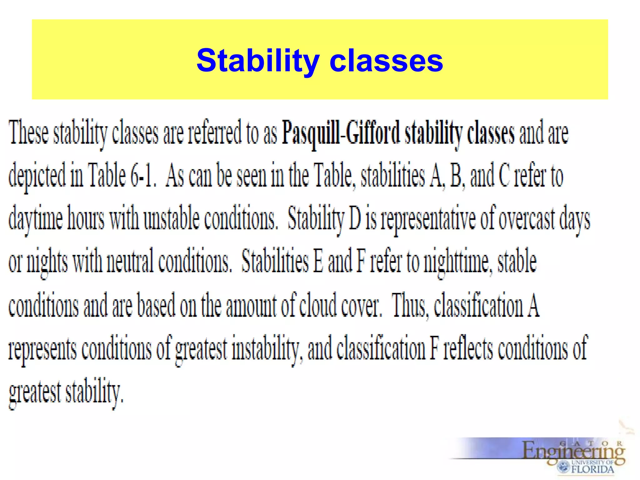
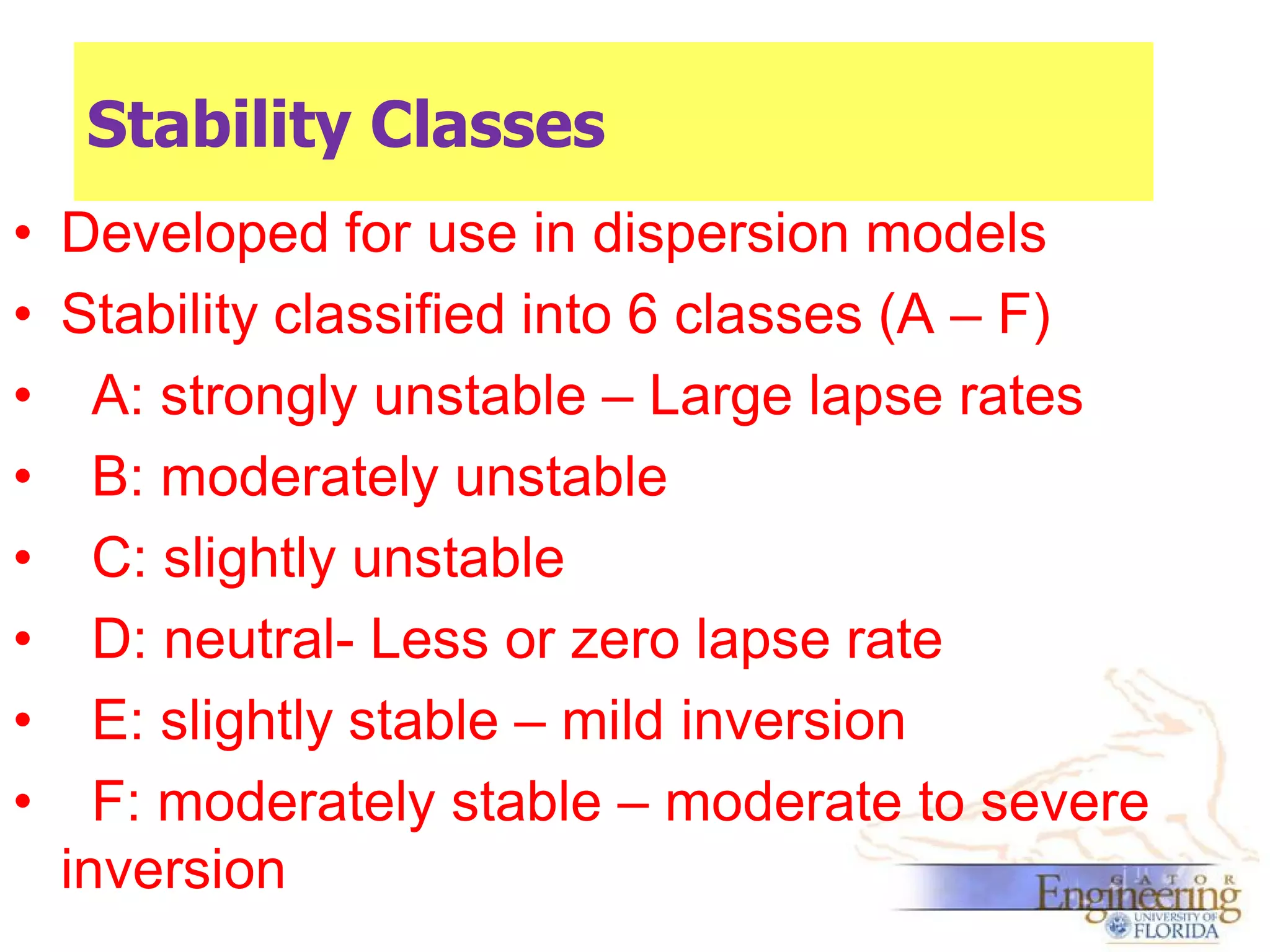
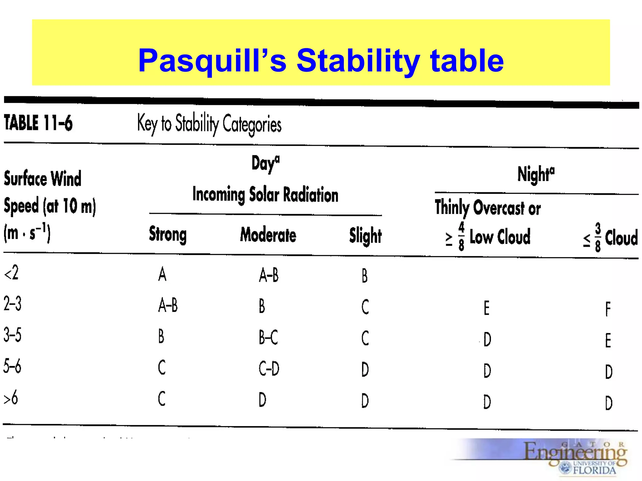
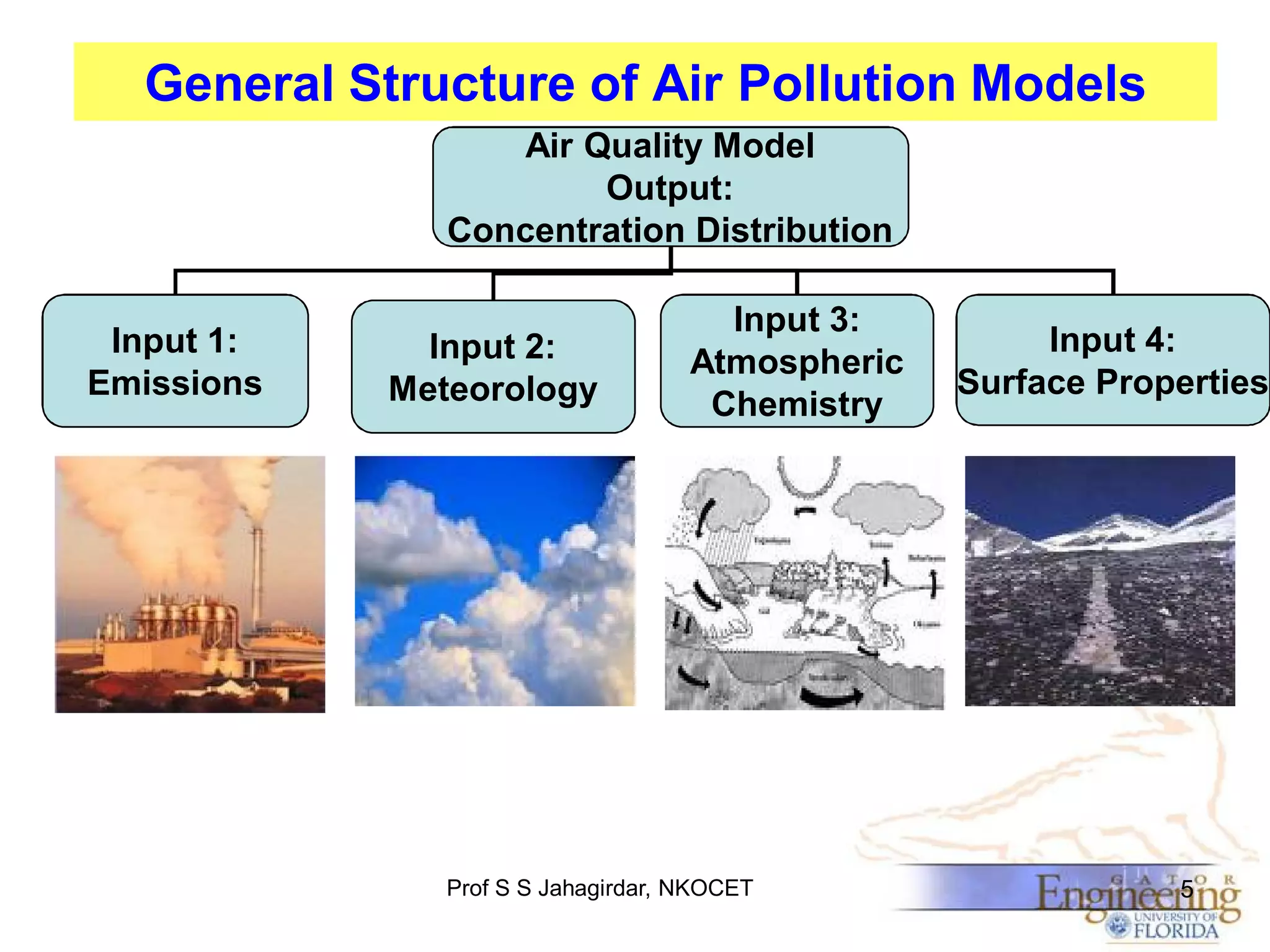
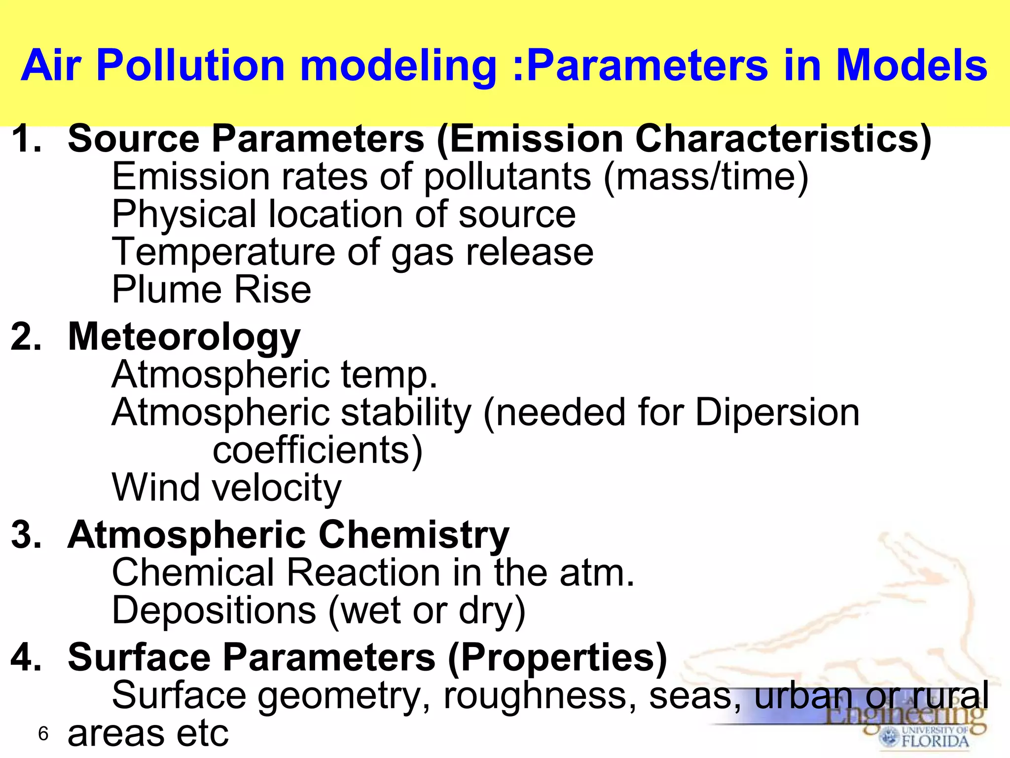
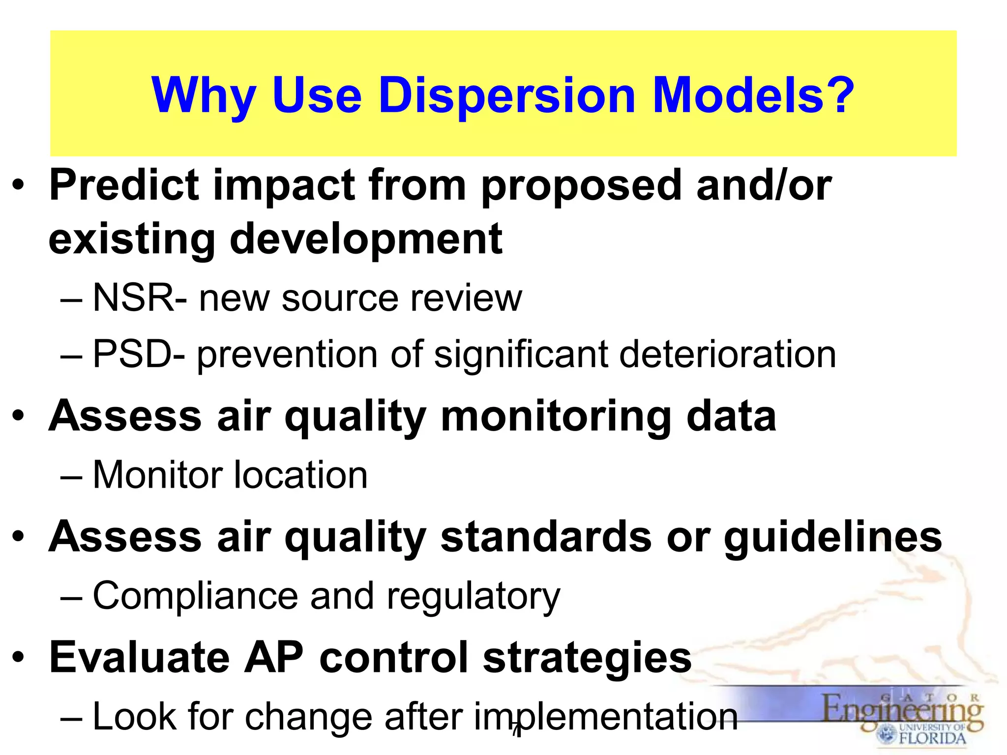
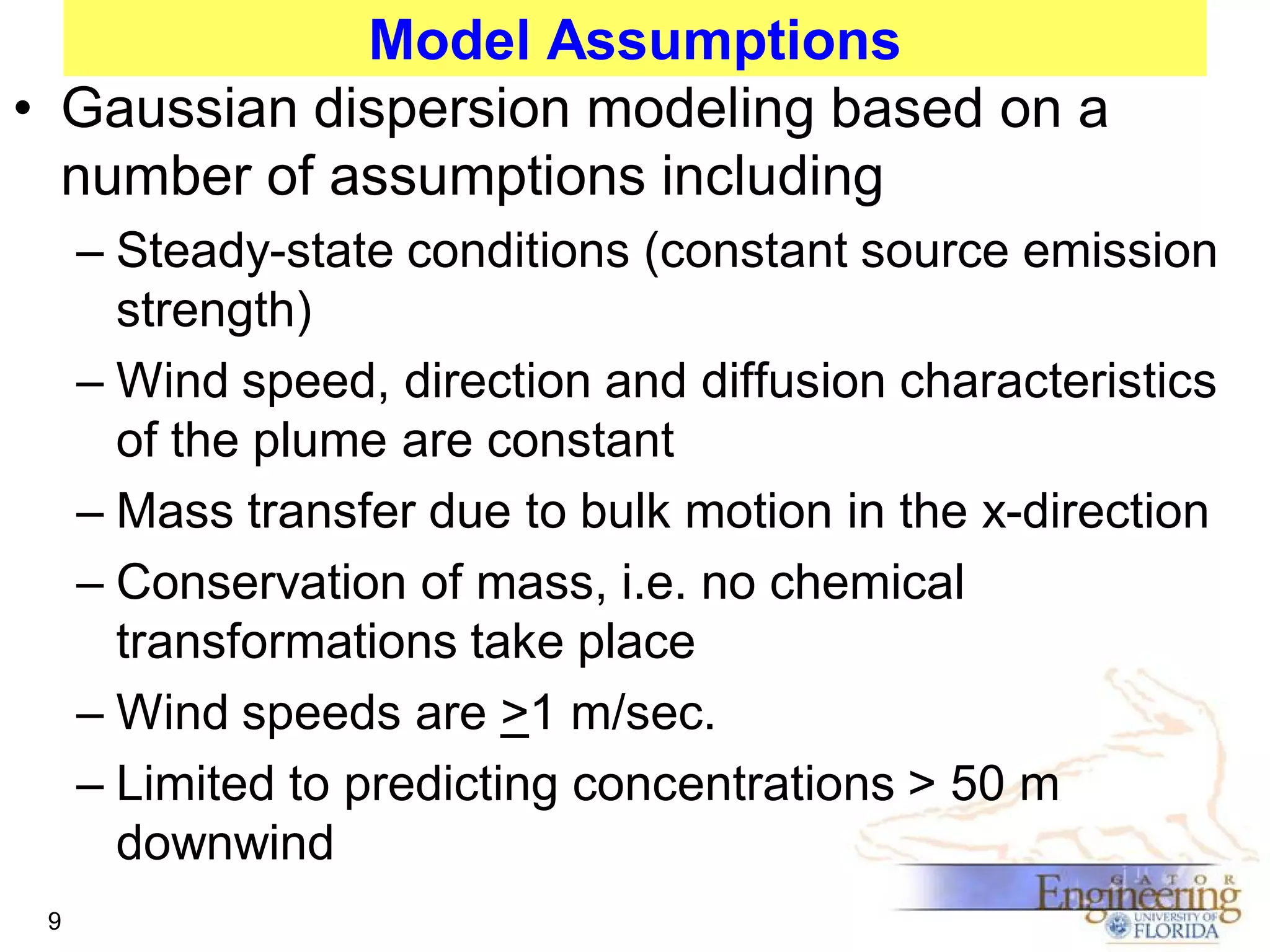
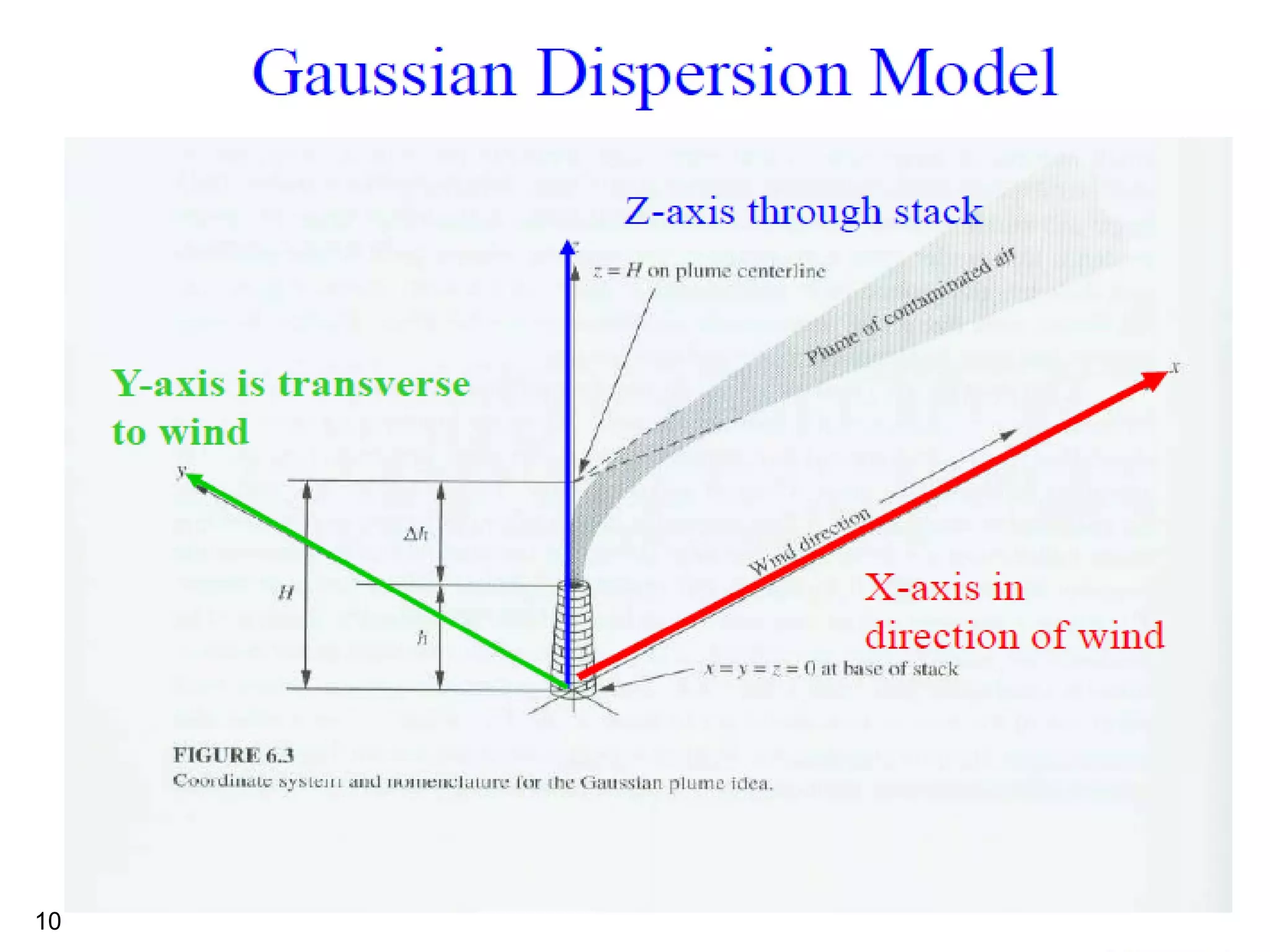
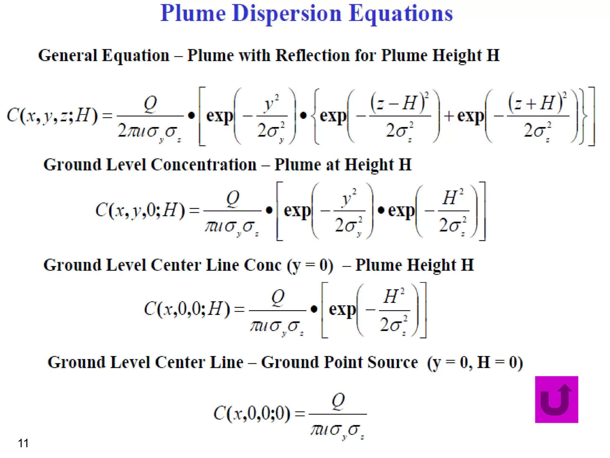
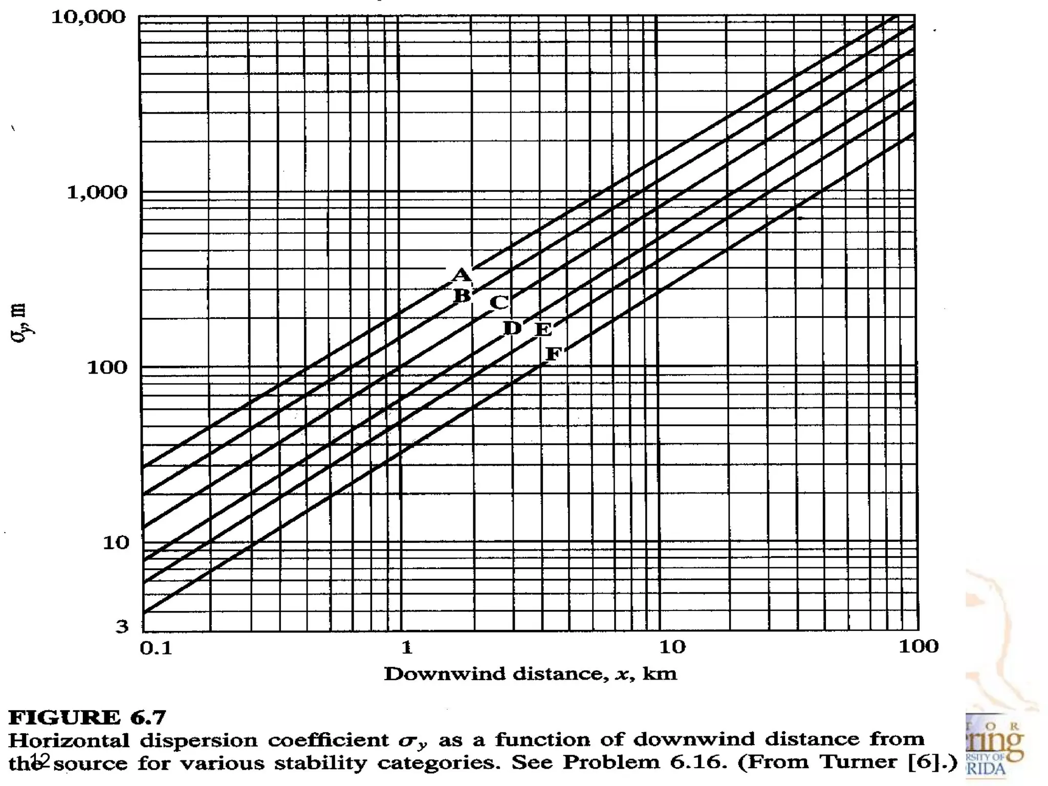
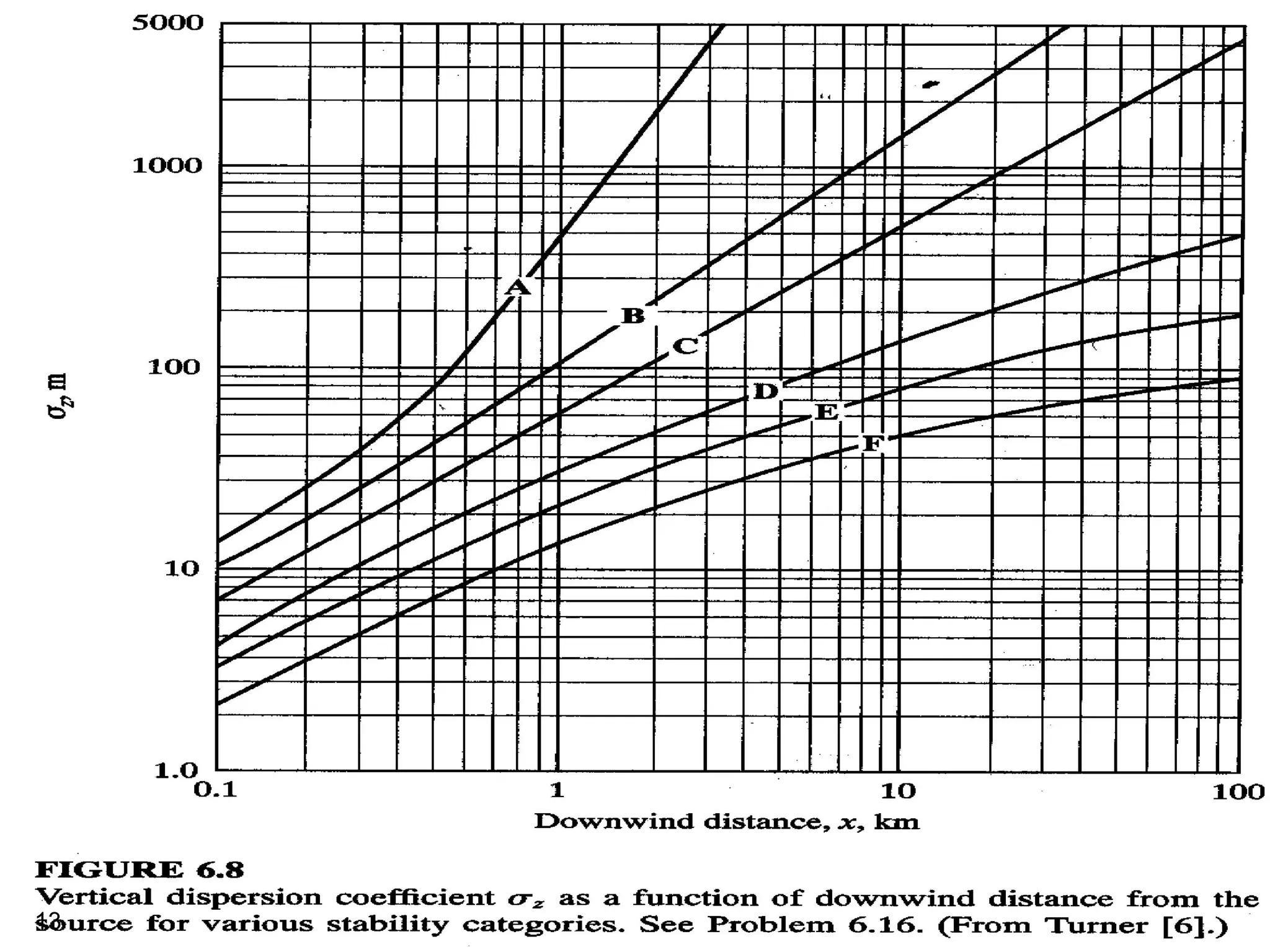
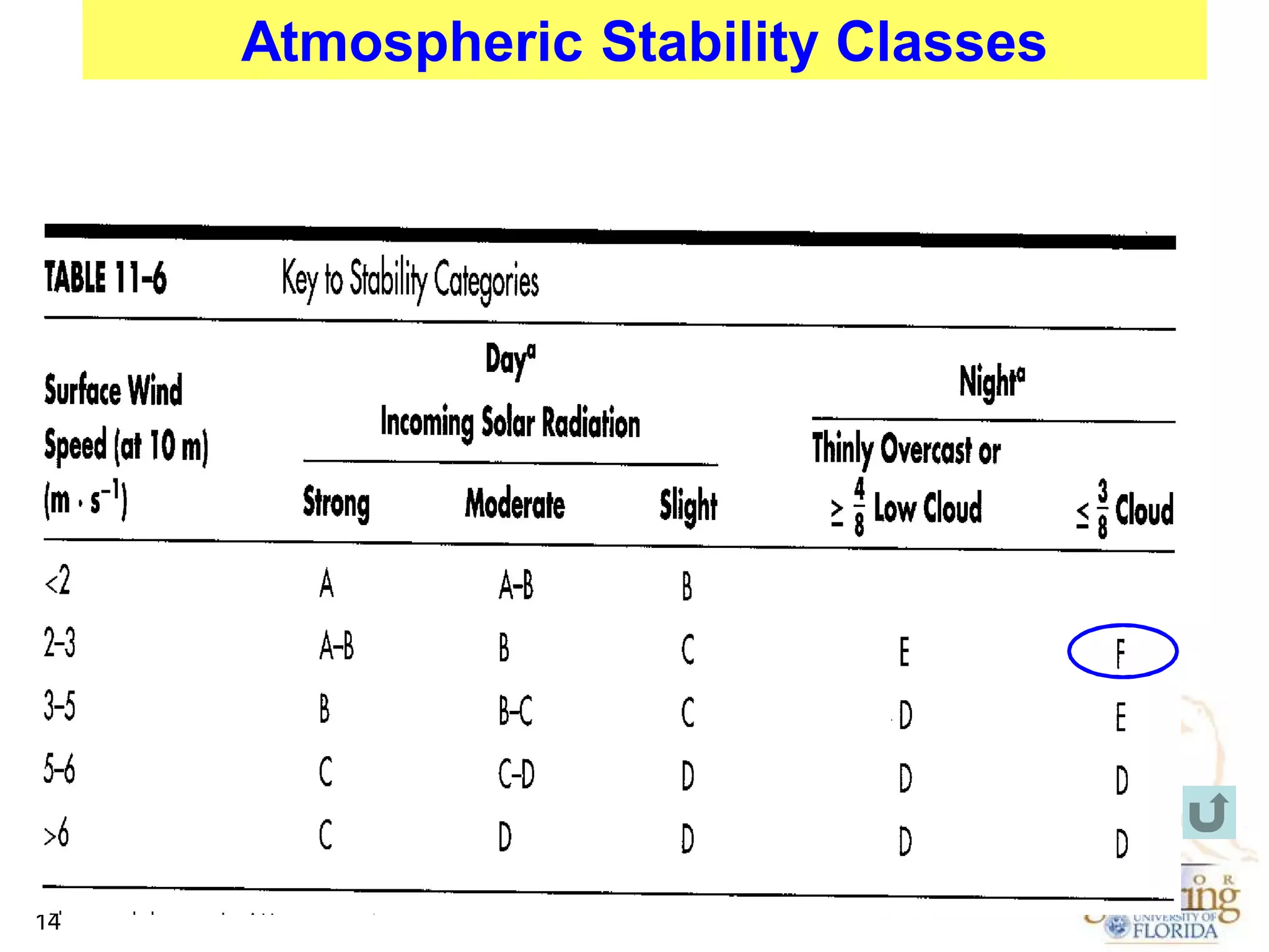
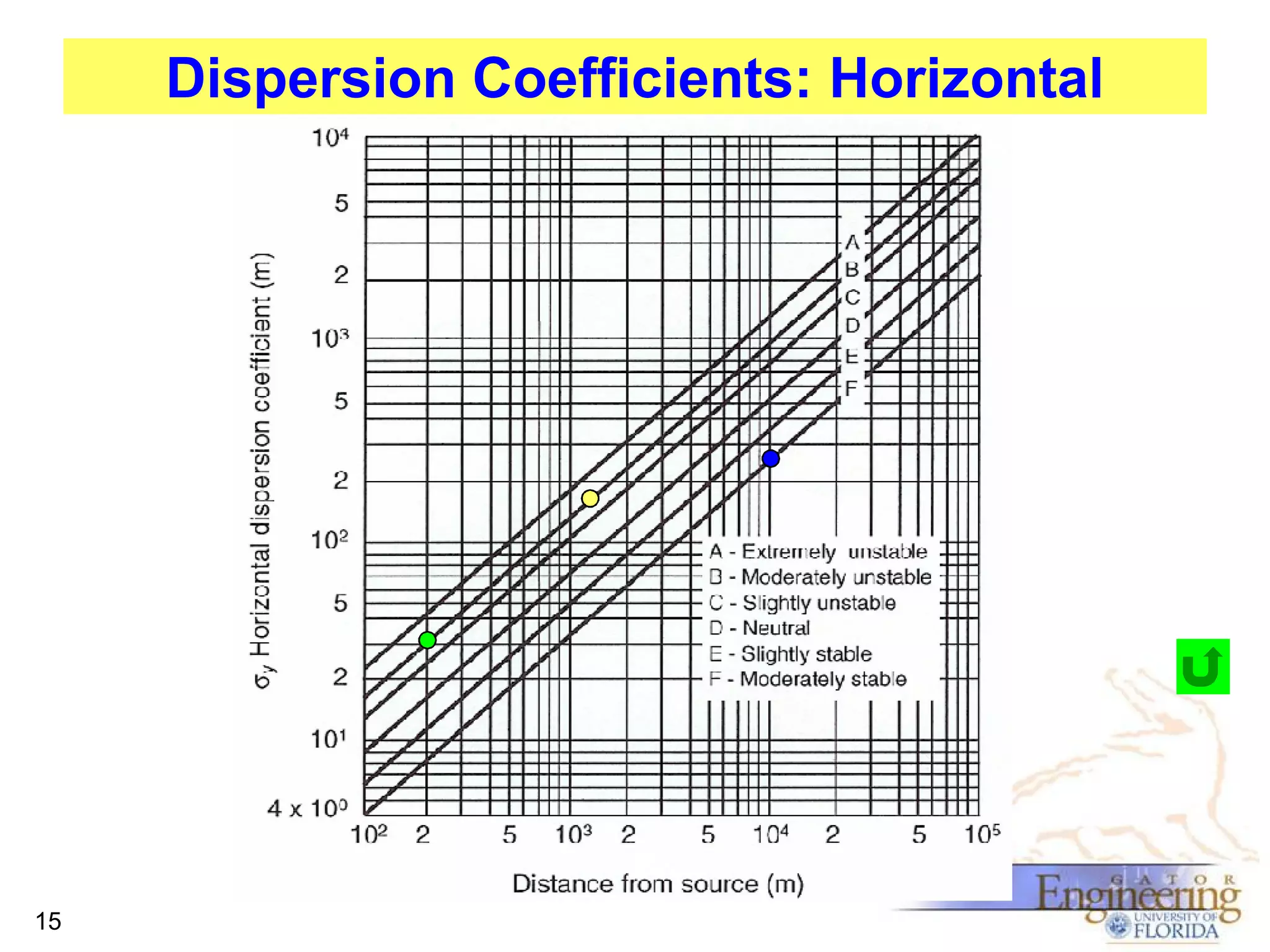
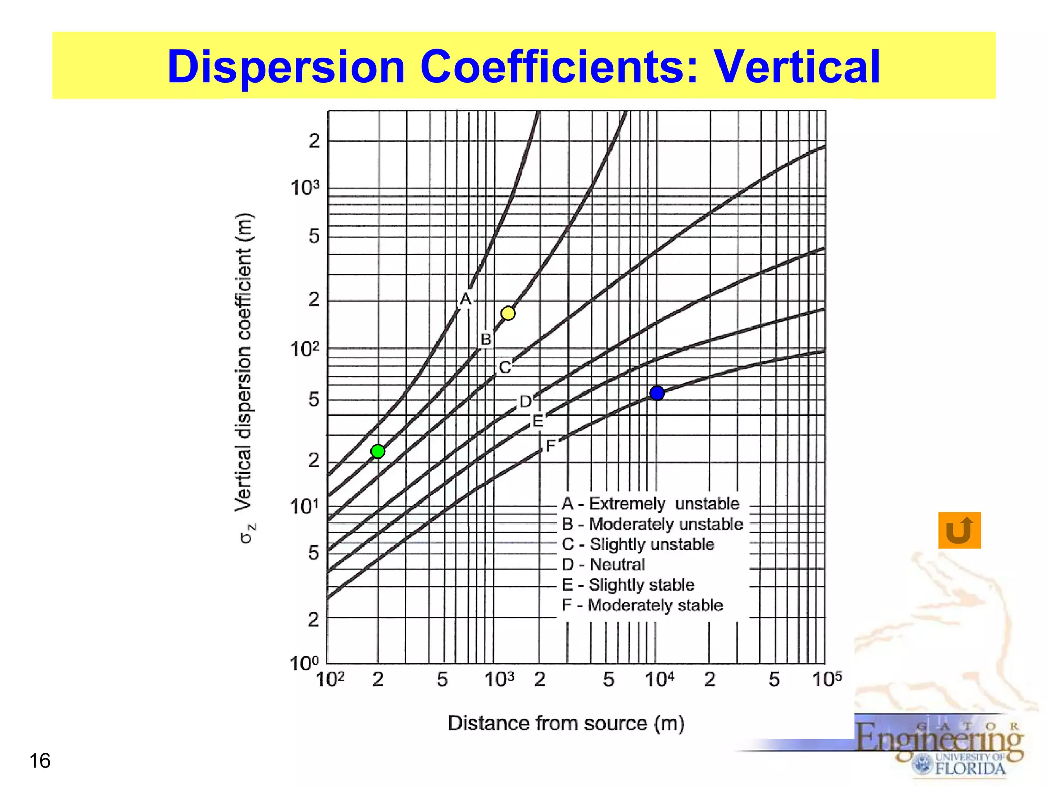
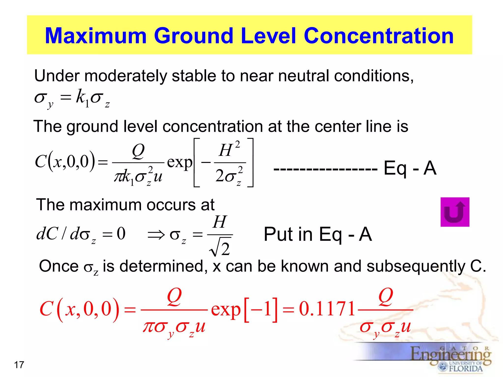
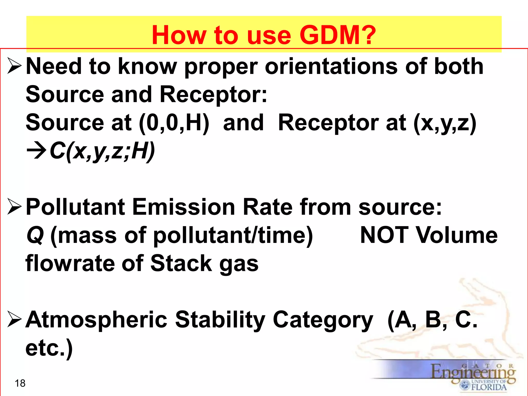
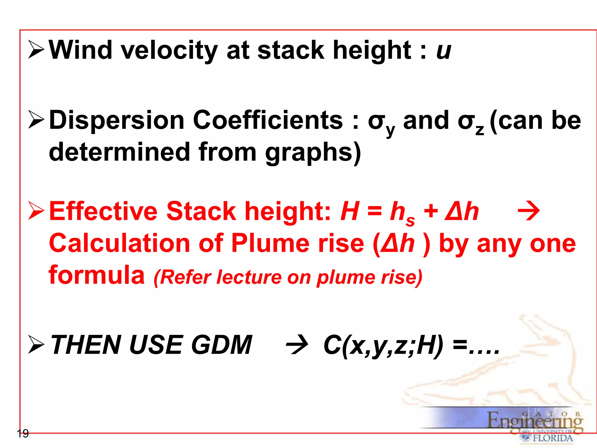
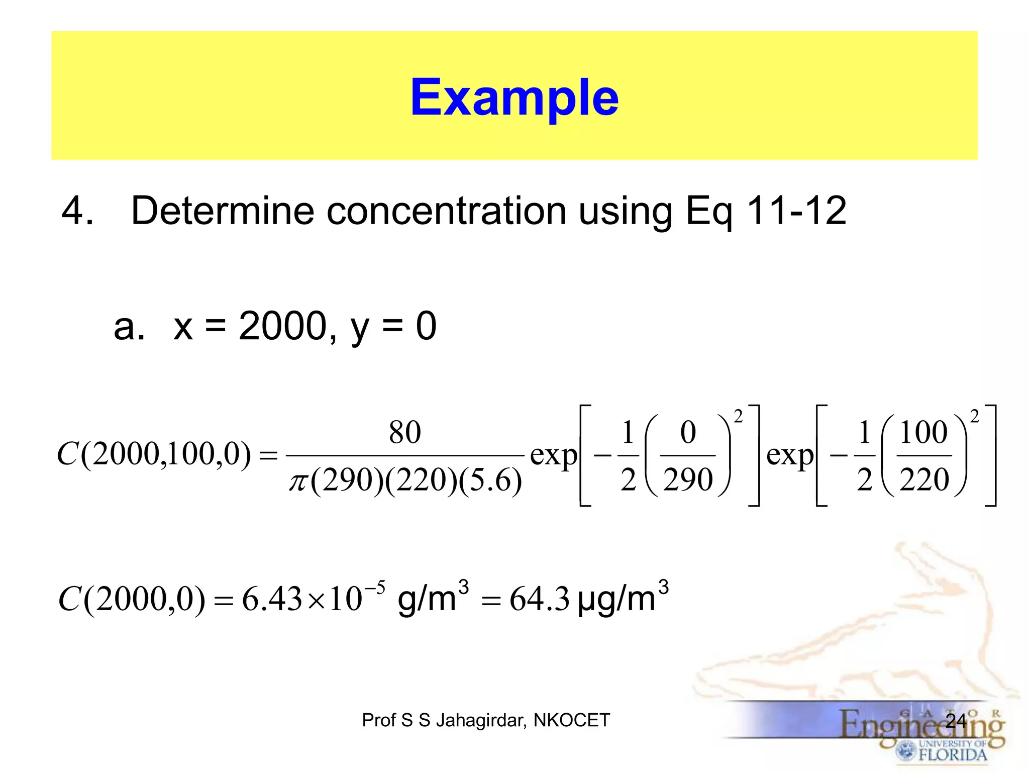
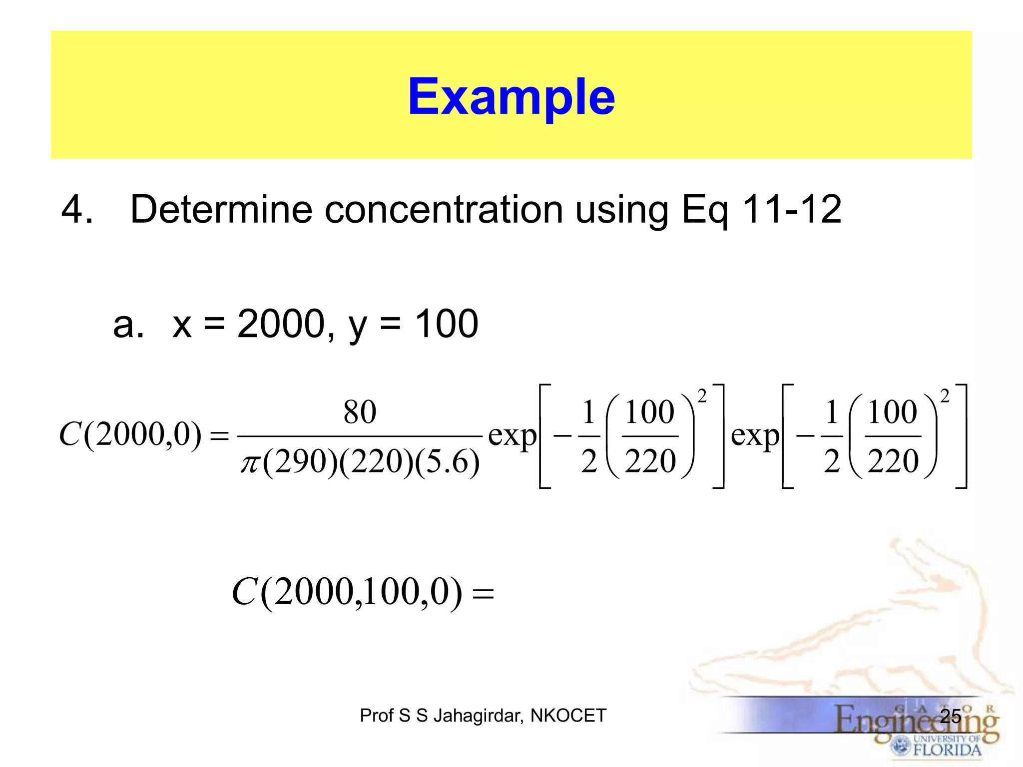
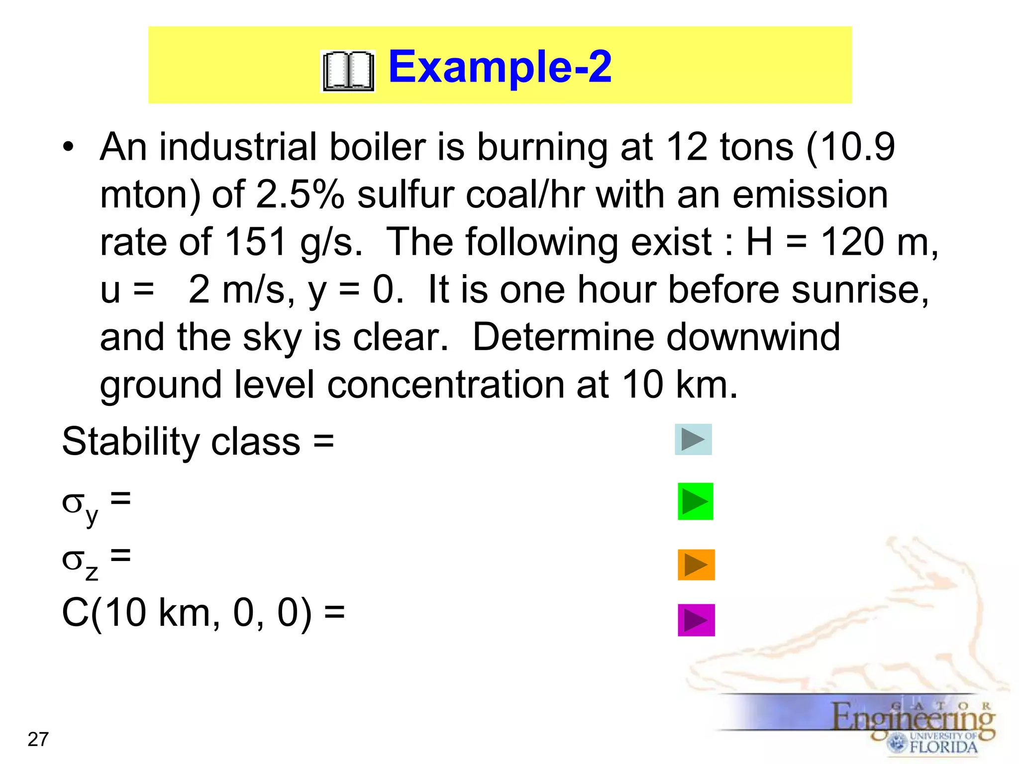
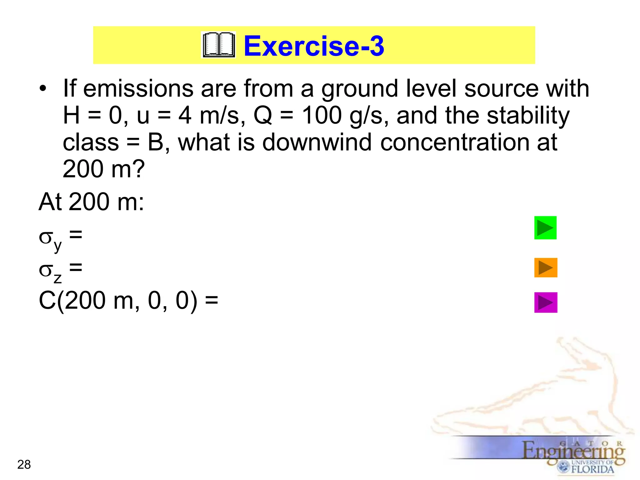
The document discusses the Gaussian Dispersion Model (GDM) used for predicting air pollution dispersion and its applications, including compliance monitoring and evaluating air quality standards. It outlines the stability classes, input parameters, model assumptions, and provides examples on how to use GDM effectively for predicting ground-level concentrations of pollutants. It concludes with exercises and theory questions to reinforce understanding of the concepts presented.

1. L-19 and L-20
Dispersion of Pollutants: Gaussian
Dispersion Model (GDM)
Air pollution and Control
(Elective -I)

2. Stability classes

3. Stability Classes
• Developed for use in dispersion models
• Stability classified into 6 classes (A – F)
• A: strongly unstable – Large lapse rates
• B: moderately unstable
• C: slightly unstable
• D: neutral- Less or zero lapse rate
• E: slightly stable – mild inversion
• F: moderately stable – moderate to severe
inversion

4. Pasquill’s Stability table

5. General Structure of Air Pollution Models
Air Quality Model
Output:
Concentration Distribution
Input 1:
Emissions
Input 2:
Meteorology
Input 3:
Atmospheric
Chemistry
Prof S S Jahagirdar, NKOCET
Input 4:
Surface Properties
5

6. Air Pollution modeling :Parameters in Models
1. Source Parameters (Emission Characteristics)
Emission rates of pollutants (mass/time)
Physical location of source
Temperature of gas release
Plume Rise
2. Meteorology
Atmospheric temp.
Atmospheric stability (needed for Dipersion
coefficients)
Wind velocity
3. Atmospheric Chemistry
Chemical Reaction in the atm.
Depositions (wet or dry)
4. Surface Parameters (Properties)
Surface geometry, roughness, seas, urban or rural
6 areas etc

7. Why Use Dispersion Models?
• Predict impact from proposed and/or
existing development
– NSR- new source review
– PSD- prevention of significant deterioration
• Assess air quality monitoring data
– Monitor location
• Assess air quality standards or guidelines
– Compliance and regulatory
• Evaluate AP control strategies
– Look for change after implementation
7

8. Why Use Dispersion Models?
• Evaluate receptor
exposure
• Monitoring network
design
– Review data
– Peak locations
– Spatial
patterns
• Model Verification
8

9. Model Assumptions
• Gaussian dispersion modeling based on a
number of assumptions including
– Steady-state conditions (constant source emission
strength)
– Wind speed, direction and diffusion characteristics
of the plume are constant
– Mass transfer due to bulk motion in the x-direction
– Conservation of mass, i.e. no chemical
transformations take place
– Wind speeds are >1 m/sec.
– Limited to predicting concentrations > 50 m
downwind
9

10. 10

11. 11

12. • Horizontal dispersion coefficient
12

13. • Vertical dispersion coefficient
13

14. Atmospheric Stability Classes
14

15. Dispersion Coefficients: Horizontal
15

16. Dispersion Coefficients: Vertical
16

17. Maximum Ground Level Concentration
Under moderately stable to near neutral conditions,
s y  k1s z
The ground level concentration at the center line is
 H2 
C x,0,0 
exp  2 
2
k1s z u
 2s z 
Q
---------------- Eq - A
The maximum occurs at
dC / ds z  0
H
 sz 
2
Put in Eq - A
Once sz is determined, x can be known and subsequently C.
C  x, 0, 0  
17
Q
s ys z u
exp  1  0.1171
Q
s ys z u

18. How to use GDM?
Need to know proper orientations of both
Source and Receptor:
Source at (0,0,H) and Receptor at (x,y,z)
C(x,y,z;H)
Pollutant Emission Rate from source:
Q (mass of pollutant/time)
NOT Volume
flowrate of Stack gas
Atmospheric Stability Category (A, B, C.
etc.)
18

19. Wind velocity at stack height : u
Dispersion Coefficients : σy and σz (can be
determined from graphs)
Effective Stack height: H = hs + Δh 
Calculation of Plume rise (Δh ) by any one
formula (Refer lecture on plume rise)
THEN USE GDM
19
 C(x,y,z;H) =….

20. Example - 1
• A stack in an urban area is emitting
80 g/s of NO. It has an effective
stack height of 100 m. The wind
speed is 4 m/s at 10 m. It is a clear
summer day with the sun nearly
overhead. Estimate the ground level
concentration at a) 2 km downwind
on the centerline and b) 2 km
downwind, 0.1 km off the centerline.
20

21. Example
1. Determine stability class
Assume wind speed is 4 km at
ground
surface.
Description
suggests strong solar radiation.
Stability class B
21

22. Example
2. Estimate the wind speed at the effective stack
height
Note: effective stack height given – no need to
calculate using Holland’s formula
p
 z2 

u 2  u1 
 z 
 1 
Prof S S Jahagirdar, NKOCET
p

 100 
4

 10 
0 .2

22

23. Example
3. Determine σy and σz
σy = 290
σz = 220
220
290
23

24. Example
4. Determine concentration using Eq 11-12
a. x = 2000, y = 0
 1  0 2 
 1  100  2 
80
C ( 2000,100,0) 
exp  
  exp  
 
 ( 290)(220)(5.6)
 2  290  
 2  220  




C ( 2000,0)  6.43 10 5 g/m3  64.3 μg/m 3
Prof S S Jahagirdar, NKOCET
24

25. Example
4. Determine concentration using Eq 11-12
a. x = 2000, y = 100
 1  100  2 
 1  100  2 
80
C ( 2000,0) 
exp  
  exp  
 
 (290)(220)(5.6)
 2  220  
 2  220  




C (2000,100,0) 
Prof S S Jahagirdar, NKOCET
25

26. L-20
Problems on GDM
Air Pollution and Control
Elective -I
Prof S S Jahagirdar, NKOCET
26

27. Example-2
• An industrial boiler is burning at 12 tons (10.9
mton) of 2.5% sulfur coal/hr with an emission
rate of 151 g/s. The following exist : H = 120 m,
u = 2 m/s, y = 0. It is one hour before sunrise,
and the sky is clear. Determine downwind
ground level concentration at 10 km.
Stability class =
sy =
sz =
C(10 km, 0, 0) =
27

28. Exercise-3
• If emissions are from a ground level source with
H = 0, u = 4 m/s, Q = 100 g/s, and the stability
class = B, what is downwind concentration at
200 m?
At 200 m:
sy =
sz =
C(200 m, 0, 0) =
28

29. Go to Additional problems
29

30. Objective Questions
Q1. GDM is used for _____________________
______________________________________.
Q2. σy and σz values depend upon __________.
Q3. In GDM ‘H’ is _________ ___________.
Q4. Greater the wind speed and mixing heights
_______________ will be the concentration of
pollutants.
Q5. Max ground level concentration is given by
_________________ .
30

31. Theory Questions
Q1. What are assumptions made in Gaussian
dispersion model?
Q2. What is Gaussian dispersion equation?
Explain meaning of each and every term in it.
Also give its different forms.
Q3. Write about how to use GDM.
Q4. What is use of Dispersion models?
Q5. Discuss parameters needed for air pollution
modeling.
31