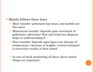
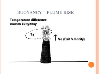
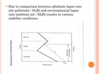
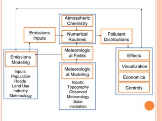
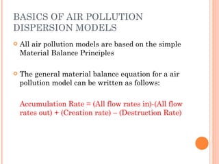
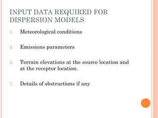
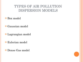
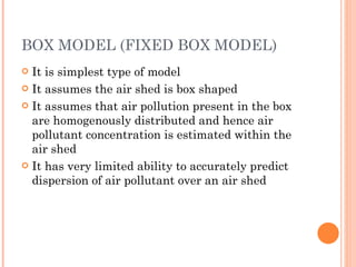
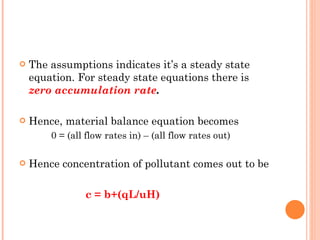
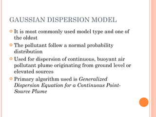
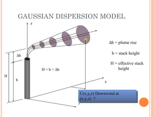
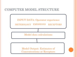
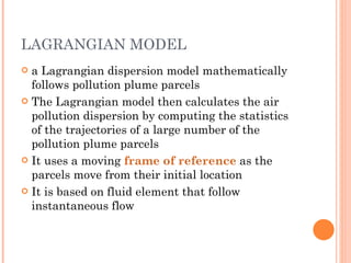
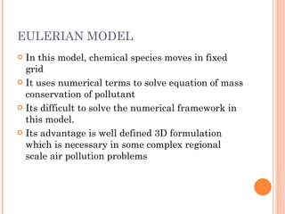
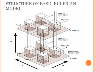
The document discusses various air pollution dispersion and modeling techniques using computers. It describes how pollutants move through mass, momentum and heat transfer processes. It then explains the basics of different modeling approaches like box models, Gaussian plume models and Eulerian/Lagrangian models. Key assumptions and equations for calculating plume rise and dispersion using Gaussian models are provided. Input requirements and structure of typical air pollution dispersion models are also summarized.

1. AIR POLLUTION DISPERSION AND MODELING USING COMPUTERS By:- KETAN WADODKAR Enroll no. 10519013 Guided by:- U.B. CHITRANSHI

2. Pollutants being harmful to human being and other living creatures And also the environmental concerns as: green house effect acid rain smog etc. AIR POLLUTION STUDY AND ITS IMPORTANCE

3. Affects visibility and also the aesthetics

4. HOW THEY MOVE / TRANSPORT OF AIR POLLUTANT BASICS

5. Mainly follows three laws: Mass transfer: pollutants has mass, and models use this mass Momentum transfer: depends upon movement of pollutants, advection= flow and wind rose diagram helps in understanding it Heat transfer: depends upon lapse rate (change of temperature / increase in height), vertical transport is convective results in heat island In case of stack monitoring all these above stated things are important

6. BUOYANCY = PLUME RISE

7. Due to comparison between adiabatic lapse rate (air pollutant / ALR) and environmental lapse rate (ambient air / ELR) results in various stability conditions

8. Inversion super adiabatic sub adiabatic Dry adiabatic lapse rate = neutral DALR

9. STABILITY AFFECTS PLUME SHAPE / PLUME BEHAVIOR

11. AIR POLLUTION DISPERSION MODELING

12. WHAT IS DISPERSION MODELING It is an attempt to describe relationship between emission, occurring concentration and deposition It gives complete analysis of what emission sources have lead to concentration depositions Mathematical models use analytical and numerical formulations, usually implemented on computers

13. WHY DISPERSION MODELING IS REQUIRED To predict ambient air concentration which will result from a emission source To plan and execute air pollution control program considering cost effectiveness For environmental impact assessment Quantify the impact of process improvements Evaluating the performance of emission control techniques Optimization of stack height, diameter Planning the control of air pollution episodes

15. Emissions Modeling Controls Economics Visualization Effects Pollutant Distributions Meteorological Fields Numerical Routines Atmospheric Chemistry Meteorological Modeling Emissions Inputs Inputs: Population Roads Land Use Industry Meteorology Inputs: Topography Observed Meteorology Solar insolation

16. BASICS OF AIR POLLUTION DISPERSION MODELS All air pollution models are based on the simple Material Balance Principles The general material balance equation for a air pollution model can be written as follows: Accumulation Rate = (All flow rates in)-(All flow rates out) + (Creation rate) – (Destruction Rate)

17. INPUT DATA REQUIRED FOR DISPERSION MODELS Meteorological conditions Emissions parameters Terrain elevations at the source location and at the receptor location. Details of obstructions if any

18. TYPES OF AIR POLLUTION DISPERSION MODELS Box model Gaussian model Lagrangian model Eulerian model Dense Gas model

19. BOX MODEL (FIXED BOX MODEL) It is simplest type of model It assumes the air shed is box shaped It assumes that air pollution present in the box are homogenously distributed and hence air pollutant concentration is estimated within the air shed It has very limited ability to accurately predict dispersion of air pollutant over an air shed

21. The assumptions indicates it’s a steady state equation. For steady state equations there is zero accumulation rate . Hence, material balance equation becomes 0 = (all flow rates in) – (all flow rates out) Hence concentration of pollutant comes out to be c = b+(qL/uH)

22. GAUSSIAN DISPERSION MODEL It is most commonly used model type and one of the oldest The pollutant follow a normal probability distribution Used for dispersion of continuous, buoyant air pollutant plume originating from ground level or elevated sources Primary algorithm used is Generalized Dispersion Equation for a Continuous Point-Source Plume

23. GAUSSIAN DISPERSION MODEL C(x,y,z) Downwind at (x,y,z) ?  h h H z x y   h = plume rise h = stack height H = effective stack height H = h +  h

24. The contaminated gas stream normally known as plume For Gaussian plume calculation the plume is assumed to be emitted from a point 0,0,H(eff). Where H(eff) is the effective stack height which is the sum of the physical stack height (hs) and the plume rise Δh To find out the dispersion of plume by the Gaussian model theory the Plume rise height has to be computed

25. MODEL ASSUMPTIONS Continuous constant pollutant emissions Conservation of mass in atmosphere No reactions occurring between pollutants When pollutants hit ground: reflected, or absorbed Steady-state meteorological conditions Short term assumption Concentration profiles are represented by Gaussian distribution—bell curve shape

26. GAUSSIAN PLUME DISPERSION One approach: assume each individual plume behaves in Gaussian manner Results in concentration profile with bell-shaped curve

27. u = wind speed Q = discharge of pollutant H = h + ∆h where, x,y = stack location z = location of interest σ z and σ y = are functions of atmospheric stability class (measure of turbulence in ambient air) h = physical stack height ∆ h = plume rise

28. FIGURE 4-3 WARK, WARNER & DAVIS Use of an imaginary source to describe reflection at the ground

29. FIGURE 4-4 WARK, WARNER & DAVIS Effect of ground reflection on pollutant concentration

30. STACK HEIGHT AND PLUME RISE BY HOLLAND'S EQUATION

31. AS GAUSSIANS MODEL REQUIRES INPUT OF H WHICH IS POLLUTANT’S PLUME CENTERLINE ABOVE GROUND LEVEL WHICH IS OBTAINED BY BRIGG'S EQUATION Here Δh = plume rise, in m F = buoyancy factor, in m4s-3 x = downwind distance from plume source, in m. xf = downwind distance from plume source to point of maximum plume rise, in m. u = wind speed at actual stack height, in m/s s = stability parameter, in s-2

32. GAUSSIAN MODEL ACCORDING TO A SOFTWARE NAMED SCREEN3

33. COMPUTER MODEL STRUCTURE INPUT DATA: Operator experience METEROLOGY EMISSIONS RECEPTORS Model Output: Estimates of Concentrations at Receptors Model does calculations

34. LAGRANGIAN MODEL a Lagrangian dispersion model mathematically follows pollution plume parcels The Lagrangian model then calculates the air pollution dispersion by computing the statistics of the trajectories of a large number of the pollution plume parcels It uses a moving frame of reference as the parcels move from their initial location It is based on fluid element that follow instantaneous flow

35. EULERIAN MODEL In this model, chemical species moves in fixed grid It uses numerical terms to solve equation of mass conservation of pollutant Its difficult to solve the numerical framework in this model. Its advantage is well defined 3D formulation which is necessary in some complex regional scale air pollution problems

36. STRUCTURE OF BASIC EULERIAN MODEL

37. DENSE GAS MODELS Dense gas model — Dense gas models are models that simulate the dispersion of dense gas pollution plumes (i.e., pollution plumes that are heavier than air). The air dispersion models used nowadays are: ADMS 3 AERMOD CALPUFF DISPERSION21 ISC3 MERCURE NAME PUFF-PLUME SIRANE Some of these models which are mentioned above are described in brief in the following slides.

38. ADMS 3 (Atmospheric dispersion modeling system) : It is an advanced model for calculating atmospheric pollutant emitted continuously (from point, line area volume source) or intermittently (from point source) AERMOD: It is steady state Gaussian plume model for short range about 50kms It uses a single wind field to transport emitted species A meteorological data preprocessor (AERMET) that accepts surface meteorological data, upper air soundings, and optionally, data from on-site instrument towers. A terrain preprocessor (AERMAP) whose main purpose is to provide a physical relationship between terrain features and the behavior of air pollution plumes

39. CALPUFF: It advanced Gaussian puff modeling system Used for longer range transport of pollutant and their effect on Federal class I areas model is designed to simulate the dispersion of buoyant, puff or continuous point and area pollution sources as well as the dispersion of buoyant, continuous line sources model also includes algorithms for handling the effect of downwash by nearby buildings in the path of the pollution plumes

40. ISC 3 : Steady state Gaussian plume model for analyzing pollutant concentration for industrial complex This model can account for the following: settling and dry deposition of particles; downwash; point, area, line, and volume sources; plume rise as a function of downwind distance; separation of point sources; and limited terrain adjustment ISC3 operates in both long-term and short-term modes

41. Puff plume: PUFF-PLUME is a model used to help predict how air pollution disperses in the atmosphere It is a Gaussian atmospheric transport chemical/radionuclide dispersion model that includes wet and dry deposition, real-time input of meteorological observations and forecasts, dose estimates from inhalation and gamma shine (i.e., radiation), and puff or continuous plume dispersion modes