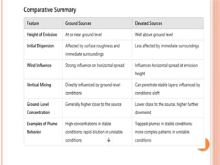
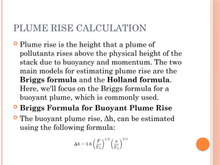
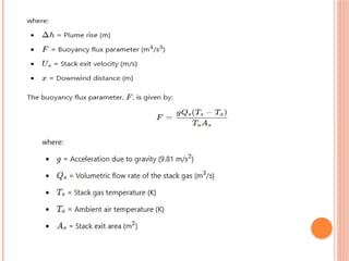
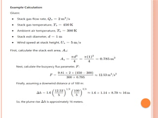
AIR POLLUTION
An overview
INTRODUCTION
 Air pollution refers to the presence of harmful or
excessive quantities of substances in the air that
pose risks to human health and the environment.
These pollutants can be in the form of gases,
particles, or biological molecules
SOURCES OF AIR POLLUTION
 Natural Sources:
• Volcanic Eruptions: Emit ash, sulfur dioxide
(SO ), and other gases.
₂
• Forest Fires: Release particulate matter (PM),
carbon monoxide (CO), and nitrogen oxides
(NO ).
ₓ
• Dust Storms: Spread fine particulate matter
over large areas.
• Biological Decay: Produces methane (CH ) and
₄
other organic compounds.
SOURCES OF AIR POLLUTION
 Anthropogenic (Human-made) Sources:
• Industrial Activities: Factories release pollutants like
sulfur dioxide (SO ), nitrogen oxides (NO ), particulate
₂ ₓ
matter (PM), and volatile organic compounds (VOCs).
• Transportation: Vehicles emit carbon monoxide (CO),
nitrogen oxides (NO ), hydrocarbons, and particulate
ₓ
matter.
• Agricultural Activities: Use of fertilizers and pesticides
releases ammonia (NH ) and other chemicals.
₃
• Burning of Fossil Fuels: Power plants and heating
systems emit sulfur dioxide (SO ), nitrogen oxides (NO ),
₂ ₓ
and carbon dioxide (CO ).
₂
• Waste Management: Landfills produce methane (CH )
₄
and other gases during decomposition.
IMPACT OF AIR POLLUTION ON THE
ENVIRONMENT IN PAKISTAN
Climate Change: Pollutants like carbon dioxide (CO ) and
₂
methane (CH ) contribute to the greenhouse effect, leading to
₄
global warming and climate change.
•Ecosystem Damage: Air pollutants can damage forests, bodies
of water, and soils, affecting plant and animal life.
•Reduction in Visibility: Smog and haze reduce visibility,
affecting daily life and transportation.
•Soil and Water Contamination: Pollutants can settle on the
ground and water bodies, contaminating them and affecting the
flora and fauna.
•Acid Rain: Emissions of sulfur dioxide (SO ) and nitrogen
₂
oxides (NO ) can lead to the formation of acid rain, which harms
ₓ
aquatic ecosystems, soil, and vegetation.
IMPACT OF AIR POLLUTION ON
HEALTH IN PAKISTAN
Respiratory Diseases: High levels of particulate matter (PM) and other
pollutants can lead to respiratory issues, including asthma, bronchitis,
and chronic obstructive pulmonary disease (COPD).
•Cardiovascular Problems: Air pollution is linked to heart diseases,
including heart attacks and strokes.
•Premature Death: Long-term exposure to polluted air can lead to
premature death due to respiratory and cardiovascular diseases.
•Cancer: Certain pollutants, like benzene and formaldehyde, are known
carcinogens and can increase the risk of cancer.
•Developmental and Reproductive Issues: Pollutants can affect fetal
development, leading to low birth weight, preterm birth, and
developmental disorders.
•Eye Irritation: Smog and other pollutants can cause eye irritation and
exacerbate conditions like conjunctivitis.
•Neurological Effects: Emerging research suggests that air pollution
may affect cognitive function and increase the risk of neurological
disorders.
SPECIFIC CHALLENGES IN
PAKISTAN
Urbanization: Rapid urbanization and industrialization have
led to increased pollution levels in major cities like Lahore,
Karachi, and Islamabad.
•Energy Production: Reliance on fossil fuels for energy
production results in significant emissions of pollutants.
•Lack of Regulation: Weak enforcement of environmental
regulations and standards exacerbates the problem.
•Public Awareness: There is limited public awareness and
education about the sources and effects of air pollution.
•Seasonal Variations: Smog in the winter months, particularly
in Punjab, is a major issue due to temperature inversions and
crop burning.
TYPES OF AIR POLLUTANTS
 Primary pollutants
 carbon monoxide
 sulfur dioxide
 nitrogen oxides
 particulate matter
 Secondary pollutants
 Ground level ozone
 smog
ATMOSPHERIC DISPERSION
 Atmospheric dispersion refers to the process by
which airborne pollutants spread and dilute in
the atmosphere. It involves the transport and
diffusion of pollutants emitted from sources such
as factories, vehicles, and natural events (like
wildfires) into the surrounding air. The
dispersion of pollutants is influenced by various
atmospheric conditions, including wind speed
and direction, temperature, humidity, and
atmospheric stability.
KEY FACTORS AFFECTING
ATMOSPHERIC DISPERSION
•Wind:
Speed: Higher wind speeds increase the dispersion of pollutants,
reducing their concentration.
•Direction: The direction of the wind determines the path that
pollutants will follow.
•Atmospheric Stability:
•Stable Atmosphere: Limits vertical mixing, often leading to
higher concentrations of pollutants near the source.
•Unstable Atmosphere: Promotes vertical mixing, dispersing
pollutants more thoroughly.
•Temperature:
•Temperature Inversions: Occur when a layer of warmer air traps
pollutants near the ground, preventing them from dispersing.
KEY FACTORS AFFECTING
ATMOSPHERIC DISPERSION
•Topography:
•Mountains and Valleys: Can channel and
concentrate pollutants in certain areas.
•Urban Structures: Buildings and other
structures can affect wind flow and pollutant
dispersion.
•Turbulence:
•Mechanical Turbulence: Caused by obstacles
such as buildings and trees disrupting airflow.
•Thermal Turbulence: Created by temperature
differences in the atmosphere, enhancing
dispersion.
MODELS OF ATMOSPHERIC
DISPERSION
 Several mathematical and computational models
are used to predict the dispersion of pollutants in
the atmosphere. These models help in assessing
the impact of emissions and planning control
strategies.
 Gaussian Plume Model:
 Lagrangian Models:
 Eulerian Models:
 Computational Fluid Dynamics (CFD)
Models
GAUSSIAN PLUME MODEL:
 The Gaussian Plume Model is one of the most
widely used mathematical models for predicting
the dispersion of pollutants released into the
atmosphere. It assumes that the distribution of
pollutant concentrations downwind of a source
follows a Gaussian, or normal, distribution both
horizontally and vertically
KEY ASSUMPTIONS
 Continuous Emission: The source emits
pollutants at a steady rate over time.
 Steady-State Conditions: Meteorological
conditions (wind speed, wind direction,
atmospheric stability) are constant during the
dispersion period.
 Gaussian Distribution: Pollutant
concentration follows a normal distribution in
both the horizontal and vertical directions from
the source.
GAUSSIAN DISTRIBUTION MODEL
EQUATION
GAUSSIAN DISTRIBUTION MODEL
PARAMETERS
Emission Rate (Q): The amount of pollutant released
per unit time.
Wind Speed (u): The speed of the wind at the
effective stack height, which influences how quickly
pollutants are transported downwind.
Effective Stack Height (H): The height at which
pollutants are effectively released into the
atmosphere, considering both the physical stack
height and the plume rise due to thermal buoyancy
and momentum.
Dispersion Coefficients (σy​and σz​
): These
coefficients depend on the atmospheric stability and
describe the spread of the plume in the horizontal and
vertical directions.
ATMOSPHERIC STABILITY CLASSES
 Atmospheric Stability Classes
 Atmospheric stability affects the dispersion coefficients
and is categorized into six classes (A-F):
• A (Very unstable)
• B (Unstable)
• C (Slightly unstable)
• D (Neutral)
• E (Slightly stable)
• F (Stable)
 Unstable conditions (A-C) promote greater dispersion,
while stable conditions (E-F) limit dispersion and can
lead to higher pollutant concentrations near the source.
APPLICATIONS
•Air Quality Management: Estimating the impact of
industrial emissions on air quality in surrounding areas.
•Regulatory Compliance: Ensuring that emissions from
facilities comply with environmental standards and
regulations.
•Emergency Response: Predicting the dispersion of
pollutants during accidental releases, such as chemical
spills or fires.
•Environmental Impact Assessments: Evaluating the
potential impact of new industrial projects on local air
quality.
ADVANTAGES AND LIMITATIONS
 Advantages:
• Simplicity: The model is relatively simple to understand and
implement.
• Efficiency: Suitable for quick assessments of pollutant dispersion
over short to moderate distances.
• Widely Used: Accepted by regulatory agencies for compliance and
impact assessment purposes.
 Limitations:
• Assumptions: The model assumes steady-state conditions and
continuous emissions, which may not always be realistic.
• Simplification: Complex terrain and varying meteorological
conditions can limit the model's accuracy.
• Distance Limitation: The model is most accurate for short to
moderate distances from the source; accuracy diminishes over long
distances.
DETERMINING ATMOSPHERIC
STABILITY CLASS
 Atmospheric stability class is a key factor in dispersion
modeling, including the Gaussian Plume Model, as it
influences the dispersion coefficients (σy and σz​
).
Stability class can be determined using several
methods, the most common of which are based on
meteorological observations and empirical methods.
 Pasquill-Gifford-Turner (PGT) Method
 Richardson Number Method
 Delta-T Method
 Monin-Obukhov Length (L)
METHODS TO DETERMINING
ATMOSPHERIC STABILITY CLASS
 Pasquill-Gifford-Turner (PGT) Method:
• The PGT method uses empirical criteria based on surface wind
speed and solar radiation (daytime) or cloud cover (nighttime).
• It classifies atmospheric conditions into six stability classes (A-F),
where A is very unstable, and F is very stable.
 Richardson Number Method:
• Uses temperature and wind profile data to compute the
Richardson number, which indicates stability.
 Delta-T Method:
• Based on the temperature difference between two levels (e.g.,
surface and a few hundred meters above the ground).
 Monin-Obukhov Length (L):
• Uses surface fluxes of heat and momentum to estimate stability.
PASQUILL-GIFFORD-TURNER (PGT)
METHOD
STEPS TO DETERMINE STABILITY
CLASS USING PGT METHOD
 Determine the Time of Day
 Measure Surface Wind Speed
 Assess Solar Radiation or Cloud Cover
 Classify Stability
MICROMETEOROLOGY
 Micrometeorology is a branch of meteorology
that focuses on the study of atmospheric
processes and phenomena at a small spatial scale
and over short time periods. It primarily deals
with the atmospheric layer closest to the Earth's
surface, typically extending up to 1-2 kilometers
above the ground. This layer is known as the
atmospheric boundary layer or the planetary
boundary layer.
SCOPE OF MICROMETEOROLOGY
 Surface-Atmosphere Interactions
 Microclimates
 Pollutant Dispersion
 Agricultural Meteorology
 Soil-Atmosphere Interactions
 Weather Forecasting
 Environmental Management
KEY CONTRIBUTIONS OF
MICROMETEOROLOGY TO ATMOSPHERIC
DISPERSION
 Characterization of the Atmospheric Boundary
Layer:
• Structure and Dynamics: Micrometeorology provides
detailed knowledge of the atmospheric boundary layer
(ABL), where most dispersion processes occur.
Understanding the structure (such as the mixed layer,
stable boundary layer, and surface layer) and dynamics
(like turbulence and vertical mixing) is essential for
accurate dispersion modeling.
• Turbulence and Mixing: Micrometeorological studies
help quantify the intensity and scales of turbulence,
which are key factors in the dispersion and dilution of
pollutants. Turbulent eddies enhance mixing, thereby
affecting the concentration and distribution of pollutants.
KEY CONTRIBUTIONS OF
MICROMETEOROLOGY TO ATMOSPHERIC
DISPERSION
 Measurement and Analysis of Micrometeorological
Variables:
• Wind Speed and Direction: Accurate measurements of
wind speed and direction at various heights within the
ABL are crucial for predicting the transport paths of
pollutants.
• Temperature and Humidity Profiles: Vertical profiles
of temperature and humidity influence stability and
stratification within the boundary layer, affecting how
pollutants disperse vertically and horizontally.
• Radiation and Energy Fluxes: Understanding surface
energy balances and radiation fluxes helps in predicting
thermal stratification and the development of temperature
inversions, which can trap pollutants near the surface.
KEY CONTRIBUTIONS OF
MICROMETEOROLOGY TO ATMOSPHERIC
DISPERSION
 Surface-Atmosphere Interactions:
• Surface Roughness: The characteristics of the
Earth's surface (e.g., vegetation, buildings,
terrain) influence turbulence and wind patterns,
thereby affecting dispersion.
• Heat and Moisture Fluxes: Exchanges of heat
and moisture between the surface and the
atmosphere impact boundary layer stability and
mixing processes.
KEY VARIABLES OF
MICROMETEOROLOGY
 Wind Speed and Direction
(Wind speed, wind direction)
 Temperature
(Air Temperature, Earth surface temp)
 Humidity
(Relative Humidity, Specific humidity, Dew Point)
 Radiation
(Solar Radiation, Longwave Radiation)
 Atmospheric Pressure
 Precipitation
KEY VARIABLES OF
MICROMETEOROLOGY
 Soil Moisture
 Heat Fluxes
(Sensible Heat Flux, Latent Heat Flux)
 Atmospheric Stability Parameters
 Cloud Cover and Type
 Vegetation and Land Use
LAPSE RATE
 The lapse rate is defined as the rate of
temperature change with respect to altitude in
the atmosphere. It is typically expressed in
degrees Celsius per kilometer (°C/km).
 Environmental Lapse Rate (ELR)
 The Environmental Lapse Rate (ELR) refers to
the actual rate of temperature decrease with
altitude in the atmosphere at a particular time
and location. It varies with atmospheric
conditions, time of day, season, and geographical
location. The average ELR is about 6.5 °C per
kilometer in the troposphere.
LAPSE RATE
 Adiabatic Lapse Rate
The Adiabatic Lapse Rate refers to the rate of
temperature change in a parcel of air as it moves
vertically in the atmosphere without exchanging
heat with its surroundings. There are two types of
adiabatic lapse rates:
 Dry Adiabatic Lapse Rate (DALR)
DALR is approximately 9.8 °C per kilometer
 Moist Adiabatic Lapse Rate (MALR)
 about 5 °C to 6 °C per
WHAT IS PLUME?
 In environmental engineering and atmospheric
science, a "plume" refers to the visible or invisible
discharge of pollutants or other materials into
the air or water from a point source, such as a
smokestack or an industrial discharge pipe.
Plume behavior is influenced by several factors,
including atmospheric stability, wind speed, and
temperature gradients. Here are the main types
of plumes:
PLUME TYPES
 Fanning Plume
• Characteristics: Horizontally spread out, occurs
under conditions of strong atmospheric stability
(inversion layer).
• Cause: Occurs when a stable atmosphere
prevents vertical mixing, causing the pollutants
to spread horizontally.
LOOPING PLUME
•Characteristics: Up-and-down oscillation, typically
observed during daytime with strong solar heating.
•Cause: Caused by unstable atmospheric conditions
with turbulent vertical mixing.
•Appearance: Loops or waves, indicating significant
vertical mixing.
CONING PLUME
•Characteristics: Cone-shaped, relatively uniform in all
directions.
•Cause: Occurs under neutral atmospheric conditions
where there is neither strong stability nor instability.
•Appearance: Symmetrical, conical shape expanding
outward as it rises
FUMIGATION PLUME
• Characteristics: Rapid downward mixing after
being trapped under a temperature inversion.
• Cause: Occurs when an inversion layer is
present aloft and is then broken by solar heating,
causing pollutants to mix downwards rapidly.
• Appearance: Initially trapped and then quickly
spreads downward, leading to high ground-level
concentrations.
LOFTING PLUME
 Lofting Plume
• Characteristics: Pollutants rise and disperse
upward with minimal downward mixing.
• Cause: Occurs when the ground-level
atmosphere is stable (inversion) but the upper
layers are unstable.
• Appearance: Plume rises and spreads upward,
remaining elevated above the ground.
TRAPPING PLUME
• Characteristics: Confined vertically between
two layers of stable air, causing horizontal
spreading.
• Cause: Occurs when pollutants are emitted into
a layer of the atmosphere that is sandwiched
between two inversion layers.
• Appearance: Horizontal spread between two
stable layers, often appearing as a band.
DISPERSION FROM DIFFERENT
SOURCE TYPES: GROUND AND
ELEVATED SOURCES
 Ground Sources
 Ground sources are emission sources located at
or near the ground level. Examples include
vehicle exhausts, small industrial processes, and
residential heating systems.
CHARACTERISTICS OF DISPERSION FROM
GROUND SOURCES
1. Initial Spread: Pollutants disperse horizontally and vertically from
the source.
2. Wind Influence: Horizontal dispersion is strongly influenced by
wind speed and direction.
3. Vertical Mixing: Vertical dispersion is affected by atmospheric
stability and turbulence. In stable conditions, vertical mixing is
limited, leading to higher concentrations near the ground.
4. Surface Roughness: Terrain and urban structures can influence
the dispersion patterns, causing more complex and variable spread.
5. Dilution: Generally, pollutants from ground sources are diluted
more quickly due to immediate interaction with the ground-level air.
 Plume Behavior Examples
• Stable Conditions: Limited vertical dispersion, pollutants remain
close to the source, creating high ground-level concentrations.
• Unstable Conditions: Enhanced vertical mixing, pollutants
disperse more quickly, leading to lower ground-level concentrations.
ELEVATED SOURCES
 Elevated sources are emission sources located
well above the ground level, such as
smokestacks, chimneys, and flares.
CHARACTERISTICS OF DISPERSION FROM
ELEVATED SOURCES
1. Initial Elevation: Pollutants are emitted at a height above the
ground, reducing immediate ground-level concentrations.
2. Plume Rise: The initial momentum and buoyancy of the emissions
can cause the plume to rise further before it begins to disperse.
3. Wind Influence: Horizontal dispersion is influenced by wind speed
and direction at the emission height.
4. Vertical Mixing: Vertical dispersion depends on atmospheric
stability. Elevated sources can penetrate stable layers, leading to
complex dispersion patterns.
5. Downwash Effects: Buildings and other structures can cause
turbulence and downwash, affecting plume behavior.
 Plume Behavior Examples
• Stable Conditions: Limited vertical mixing can trap pollutants at
higher altitudes, creating a fanning plume.
• Unstable Conditions: Enhanced vertical mixing disperses pollutants
over a larger volume, potentially leading to looping or coning plumes.
PLUME RISE CALCULATION
 Plume rise is the height that a plume of
pollutants rises above the physical height of the
stack due to buoyancy and momentum. The two
main models for estimating plume rise are the
Briggs formula and the Holland formula.
Here, we'll focus on the Briggs formula for a
buoyant plume, which is commonly used.
 Briggs Formula for Buoyant Plume Rise
 The buoyant plume rise, Δh, can be estimated
using the following formula:
Air pollution an overview and management s

Air pollution an overview and management s

  • 1.
  • 2.
    INTRODUCTION  Air pollutionrefers to the presence of harmful or excessive quantities of substances in the air that pose risks to human health and the environment. These pollutants can be in the form of gases, particles, or biological molecules
  • 3.
    SOURCES OF AIRPOLLUTION  Natural Sources: • Volcanic Eruptions: Emit ash, sulfur dioxide (SO ), and other gases. ₂ • Forest Fires: Release particulate matter (PM), carbon monoxide (CO), and nitrogen oxides (NO ). ₓ • Dust Storms: Spread fine particulate matter over large areas. • Biological Decay: Produces methane (CH ) and ₄ other organic compounds.
  • 4.
    SOURCES OF AIRPOLLUTION  Anthropogenic (Human-made) Sources: • Industrial Activities: Factories release pollutants like sulfur dioxide (SO ), nitrogen oxides (NO ), particulate ₂ ₓ matter (PM), and volatile organic compounds (VOCs). • Transportation: Vehicles emit carbon monoxide (CO), nitrogen oxides (NO ), hydrocarbons, and particulate ₓ matter. • Agricultural Activities: Use of fertilizers and pesticides releases ammonia (NH ) and other chemicals. ₃ • Burning of Fossil Fuels: Power plants and heating systems emit sulfur dioxide (SO ), nitrogen oxides (NO ), ₂ ₓ and carbon dioxide (CO ). ₂ • Waste Management: Landfills produce methane (CH ) ₄ and other gases during decomposition.
  • 5.
    IMPACT OF AIRPOLLUTION ON THE ENVIRONMENT IN PAKISTAN Climate Change: Pollutants like carbon dioxide (CO ) and ₂ methane (CH ) contribute to the greenhouse effect, leading to ₄ global warming and climate change. •Ecosystem Damage: Air pollutants can damage forests, bodies of water, and soils, affecting plant and animal life. •Reduction in Visibility: Smog and haze reduce visibility, affecting daily life and transportation. •Soil and Water Contamination: Pollutants can settle on the ground and water bodies, contaminating them and affecting the flora and fauna. •Acid Rain: Emissions of sulfur dioxide (SO ) and nitrogen ₂ oxides (NO ) can lead to the formation of acid rain, which harms ₓ aquatic ecosystems, soil, and vegetation.
  • 6.
    IMPACT OF AIRPOLLUTION ON HEALTH IN PAKISTAN Respiratory Diseases: High levels of particulate matter (PM) and other pollutants can lead to respiratory issues, including asthma, bronchitis, and chronic obstructive pulmonary disease (COPD). •Cardiovascular Problems: Air pollution is linked to heart diseases, including heart attacks and strokes. •Premature Death: Long-term exposure to polluted air can lead to premature death due to respiratory and cardiovascular diseases. •Cancer: Certain pollutants, like benzene and formaldehyde, are known carcinogens and can increase the risk of cancer. •Developmental and Reproductive Issues: Pollutants can affect fetal development, leading to low birth weight, preterm birth, and developmental disorders. •Eye Irritation: Smog and other pollutants can cause eye irritation and exacerbate conditions like conjunctivitis. •Neurological Effects: Emerging research suggests that air pollution may affect cognitive function and increase the risk of neurological disorders.
  • 7.
    SPECIFIC CHALLENGES IN PAKISTAN Urbanization:Rapid urbanization and industrialization have led to increased pollution levels in major cities like Lahore, Karachi, and Islamabad. •Energy Production: Reliance on fossil fuels for energy production results in significant emissions of pollutants. •Lack of Regulation: Weak enforcement of environmental regulations and standards exacerbates the problem. •Public Awareness: There is limited public awareness and education about the sources and effects of air pollution. •Seasonal Variations: Smog in the winter months, particularly in Punjab, is a major issue due to temperature inversions and crop burning.
  • 8.
    TYPES OF AIRPOLLUTANTS  Primary pollutants  carbon monoxide  sulfur dioxide  nitrogen oxides  particulate matter  Secondary pollutants  Ground level ozone  smog
  • 9.
    ATMOSPHERIC DISPERSION  Atmosphericdispersion refers to the process by which airborne pollutants spread and dilute in the atmosphere. It involves the transport and diffusion of pollutants emitted from sources such as factories, vehicles, and natural events (like wildfires) into the surrounding air. The dispersion of pollutants is influenced by various atmospheric conditions, including wind speed and direction, temperature, humidity, and atmospheric stability.
  • 10.
    KEY FACTORS AFFECTING ATMOSPHERICDISPERSION •Wind: Speed: Higher wind speeds increase the dispersion of pollutants, reducing their concentration. •Direction: The direction of the wind determines the path that pollutants will follow. •Atmospheric Stability: •Stable Atmosphere: Limits vertical mixing, often leading to higher concentrations of pollutants near the source. •Unstable Atmosphere: Promotes vertical mixing, dispersing pollutants more thoroughly. •Temperature: •Temperature Inversions: Occur when a layer of warmer air traps pollutants near the ground, preventing them from dispersing.
  • 11.
    KEY FACTORS AFFECTING ATMOSPHERICDISPERSION •Topography: •Mountains and Valleys: Can channel and concentrate pollutants in certain areas. •Urban Structures: Buildings and other structures can affect wind flow and pollutant dispersion. •Turbulence: •Mechanical Turbulence: Caused by obstacles such as buildings and trees disrupting airflow. •Thermal Turbulence: Created by temperature differences in the atmosphere, enhancing dispersion.
  • 12.
    MODELS OF ATMOSPHERIC DISPERSION Several mathematical and computational models are used to predict the dispersion of pollutants in the atmosphere. These models help in assessing the impact of emissions and planning control strategies.  Gaussian Plume Model:  Lagrangian Models:  Eulerian Models:  Computational Fluid Dynamics (CFD) Models
  • 13.
    GAUSSIAN PLUME MODEL: The Gaussian Plume Model is one of the most widely used mathematical models for predicting the dispersion of pollutants released into the atmosphere. It assumes that the distribution of pollutant concentrations downwind of a source follows a Gaussian, or normal, distribution both horizontally and vertically
  • 14.
    KEY ASSUMPTIONS  ContinuousEmission: The source emits pollutants at a steady rate over time.  Steady-State Conditions: Meteorological conditions (wind speed, wind direction, atmospheric stability) are constant during the dispersion period.  Gaussian Distribution: Pollutant concentration follows a normal distribution in both the horizontal and vertical directions from the source.
  • 15.
  • 16.
    GAUSSIAN DISTRIBUTION MODEL PARAMETERS EmissionRate (Q): The amount of pollutant released per unit time. Wind Speed (u): The speed of the wind at the effective stack height, which influences how quickly pollutants are transported downwind. Effective Stack Height (H): The height at which pollutants are effectively released into the atmosphere, considering both the physical stack height and the plume rise due to thermal buoyancy and momentum. Dispersion Coefficients (σy​and σz​ ): These coefficients depend on the atmospheric stability and describe the spread of the plume in the horizontal and vertical directions.
  • 17.
    ATMOSPHERIC STABILITY CLASSES Atmospheric Stability Classes  Atmospheric stability affects the dispersion coefficients and is categorized into six classes (A-F): • A (Very unstable) • B (Unstable) • C (Slightly unstable) • D (Neutral) • E (Slightly stable) • F (Stable)  Unstable conditions (A-C) promote greater dispersion, while stable conditions (E-F) limit dispersion and can lead to higher pollutant concentrations near the source.
  • 18.
    APPLICATIONS •Air Quality Management:Estimating the impact of industrial emissions on air quality in surrounding areas. •Regulatory Compliance: Ensuring that emissions from facilities comply with environmental standards and regulations. •Emergency Response: Predicting the dispersion of pollutants during accidental releases, such as chemical spills or fires. •Environmental Impact Assessments: Evaluating the potential impact of new industrial projects on local air quality.
  • 19.
    ADVANTAGES AND LIMITATIONS Advantages: • Simplicity: The model is relatively simple to understand and implement. • Efficiency: Suitable for quick assessments of pollutant dispersion over short to moderate distances. • Widely Used: Accepted by regulatory agencies for compliance and impact assessment purposes.  Limitations: • Assumptions: The model assumes steady-state conditions and continuous emissions, which may not always be realistic. • Simplification: Complex terrain and varying meteorological conditions can limit the model's accuracy. • Distance Limitation: The model is most accurate for short to moderate distances from the source; accuracy diminishes over long distances.
  • 20.
    DETERMINING ATMOSPHERIC STABILITY CLASS Atmospheric stability class is a key factor in dispersion modeling, including the Gaussian Plume Model, as it influences the dispersion coefficients (σy and σz​ ). Stability class can be determined using several methods, the most common of which are based on meteorological observations and empirical methods.  Pasquill-Gifford-Turner (PGT) Method  Richardson Number Method  Delta-T Method  Monin-Obukhov Length (L)
  • 21.
    METHODS TO DETERMINING ATMOSPHERICSTABILITY CLASS  Pasquill-Gifford-Turner (PGT) Method: • The PGT method uses empirical criteria based on surface wind speed and solar radiation (daytime) or cloud cover (nighttime). • It classifies atmospheric conditions into six stability classes (A-F), where A is very unstable, and F is very stable.  Richardson Number Method: • Uses temperature and wind profile data to compute the Richardson number, which indicates stability.  Delta-T Method: • Based on the temperature difference between two levels (e.g., surface and a few hundred meters above the ground).  Monin-Obukhov Length (L): • Uses surface fluxes of heat and momentum to estimate stability.
  • 22.
  • 23.
    STEPS TO DETERMINESTABILITY CLASS USING PGT METHOD  Determine the Time of Day  Measure Surface Wind Speed  Assess Solar Radiation or Cloud Cover  Classify Stability
  • 24.
    MICROMETEOROLOGY  Micrometeorology isa branch of meteorology that focuses on the study of atmospheric processes and phenomena at a small spatial scale and over short time periods. It primarily deals with the atmospheric layer closest to the Earth's surface, typically extending up to 1-2 kilometers above the ground. This layer is known as the atmospheric boundary layer or the planetary boundary layer.
  • 25.
    SCOPE OF MICROMETEOROLOGY Surface-Atmosphere Interactions  Microclimates  Pollutant Dispersion  Agricultural Meteorology  Soil-Atmosphere Interactions  Weather Forecasting  Environmental Management
  • 26.
    KEY CONTRIBUTIONS OF MICROMETEOROLOGYTO ATMOSPHERIC DISPERSION  Characterization of the Atmospheric Boundary Layer: • Structure and Dynamics: Micrometeorology provides detailed knowledge of the atmospheric boundary layer (ABL), where most dispersion processes occur. Understanding the structure (such as the mixed layer, stable boundary layer, and surface layer) and dynamics (like turbulence and vertical mixing) is essential for accurate dispersion modeling. • Turbulence and Mixing: Micrometeorological studies help quantify the intensity and scales of turbulence, which are key factors in the dispersion and dilution of pollutants. Turbulent eddies enhance mixing, thereby affecting the concentration and distribution of pollutants.
  • 27.
    KEY CONTRIBUTIONS OF MICROMETEOROLOGYTO ATMOSPHERIC DISPERSION  Measurement and Analysis of Micrometeorological Variables: • Wind Speed and Direction: Accurate measurements of wind speed and direction at various heights within the ABL are crucial for predicting the transport paths of pollutants. • Temperature and Humidity Profiles: Vertical profiles of temperature and humidity influence stability and stratification within the boundary layer, affecting how pollutants disperse vertically and horizontally. • Radiation and Energy Fluxes: Understanding surface energy balances and radiation fluxes helps in predicting thermal stratification and the development of temperature inversions, which can trap pollutants near the surface.
  • 28.
    KEY CONTRIBUTIONS OF MICROMETEOROLOGYTO ATMOSPHERIC DISPERSION  Surface-Atmosphere Interactions: • Surface Roughness: The characteristics of the Earth's surface (e.g., vegetation, buildings, terrain) influence turbulence and wind patterns, thereby affecting dispersion. • Heat and Moisture Fluxes: Exchanges of heat and moisture between the surface and the atmosphere impact boundary layer stability and mixing processes.
  • 29.
    KEY VARIABLES OF MICROMETEOROLOGY Wind Speed and Direction (Wind speed, wind direction)  Temperature (Air Temperature, Earth surface temp)  Humidity (Relative Humidity, Specific humidity, Dew Point)  Radiation (Solar Radiation, Longwave Radiation)  Atmospheric Pressure  Precipitation
  • 30.
    KEY VARIABLES OF MICROMETEOROLOGY Soil Moisture  Heat Fluxes (Sensible Heat Flux, Latent Heat Flux)  Atmospheric Stability Parameters  Cloud Cover and Type  Vegetation and Land Use
  • 31.
    LAPSE RATE  Thelapse rate is defined as the rate of temperature change with respect to altitude in the atmosphere. It is typically expressed in degrees Celsius per kilometer (°C/km).  Environmental Lapse Rate (ELR)  The Environmental Lapse Rate (ELR) refers to the actual rate of temperature decrease with altitude in the atmosphere at a particular time and location. It varies with atmospheric conditions, time of day, season, and geographical location. The average ELR is about 6.5 °C per kilometer in the troposphere.
  • 32.
    LAPSE RATE  AdiabaticLapse Rate The Adiabatic Lapse Rate refers to the rate of temperature change in a parcel of air as it moves vertically in the atmosphere without exchanging heat with its surroundings. There are two types of adiabatic lapse rates:  Dry Adiabatic Lapse Rate (DALR) DALR is approximately 9.8 °C per kilometer  Moist Adiabatic Lapse Rate (MALR)  about 5 °C to 6 °C per
  • 33.
    WHAT IS PLUME? In environmental engineering and atmospheric science, a "plume" refers to the visible or invisible discharge of pollutants or other materials into the air or water from a point source, such as a smokestack or an industrial discharge pipe. Plume behavior is influenced by several factors, including atmospheric stability, wind speed, and temperature gradients. Here are the main types of plumes:
  • 34.
    PLUME TYPES  FanningPlume • Characteristics: Horizontally spread out, occurs under conditions of strong atmospheric stability (inversion layer). • Cause: Occurs when a stable atmosphere prevents vertical mixing, causing the pollutants to spread horizontally.
  • 36.
    LOOPING PLUME •Characteristics: Up-and-downoscillation, typically observed during daytime with strong solar heating. •Cause: Caused by unstable atmospheric conditions with turbulent vertical mixing. •Appearance: Loops or waves, indicating significant vertical mixing.
  • 37.
    CONING PLUME •Characteristics: Cone-shaped,relatively uniform in all directions. •Cause: Occurs under neutral atmospheric conditions where there is neither strong stability nor instability. •Appearance: Symmetrical, conical shape expanding outward as it rises
  • 38.
    FUMIGATION PLUME • Characteristics:Rapid downward mixing after being trapped under a temperature inversion. • Cause: Occurs when an inversion layer is present aloft and is then broken by solar heating, causing pollutants to mix downwards rapidly. • Appearance: Initially trapped and then quickly spreads downward, leading to high ground-level concentrations.
  • 39.
    LOFTING PLUME  LoftingPlume • Characteristics: Pollutants rise and disperse upward with minimal downward mixing. • Cause: Occurs when the ground-level atmosphere is stable (inversion) but the upper layers are unstable. • Appearance: Plume rises and spreads upward, remaining elevated above the ground.
  • 40.
    TRAPPING PLUME • Characteristics:Confined vertically between two layers of stable air, causing horizontal spreading. • Cause: Occurs when pollutants are emitted into a layer of the atmosphere that is sandwiched between two inversion layers. • Appearance: Horizontal spread between two stable layers, often appearing as a band.
  • 42.
    DISPERSION FROM DIFFERENT SOURCETYPES: GROUND AND ELEVATED SOURCES  Ground Sources  Ground sources are emission sources located at or near the ground level. Examples include vehicle exhausts, small industrial processes, and residential heating systems.
  • 43.
    CHARACTERISTICS OF DISPERSIONFROM GROUND SOURCES 1. Initial Spread: Pollutants disperse horizontally and vertically from the source. 2. Wind Influence: Horizontal dispersion is strongly influenced by wind speed and direction. 3. Vertical Mixing: Vertical dispersion is affected by atmospheric stability and turbulence. In stable conditions, vertical mixing is limited, leading to higher concentrations near the ground. 4. Surface Roughness: Terrain and urban structures can influence the dispersion patterns, causing more complex and variable spread. 5. Dilution: Generally, pollutants from ground sources are diluted more quickly due to immediate interaction with the ground-level air.  Plume Behavior Examples • Stable Conditions: Limited vertical dispersion, pollutants remain close to the source, creating high ground-level concentrations. • Unstable Conditions: Enhanced vertical mixing, pollutants disperse more quickly, leading to lower ground-level concentrations.
  • 44.
    ELEVATED SOURCES  Elevatedsources are emission sources located well above the ground level, such as smokestacks, chimneys, and flares.
  • 45.
    CHARACTERISTICS OF DISPERSIONFROM ELEVATED SOURCES 1. Initial Elevation: Pollutants are emitted at a height above the ground, reducing immediate ground-level concentrations. 2. Plume Rise: The initial momentum and buoyancy of the emissions can cause the plume to rise further before it begins to disperse. 3. Wind Influence: Horizontal dispersion is influenced by wind speed and direction at the emission height. 4. Vertical Mixing: Vertical dispersion depends on atmospheric stability. Elevated sources can penetrate stable layers, leading to complex dispersion patterns. 5. Downwash Effects: Buildings and other structures can cause turbulence and downwash, affecting plume behavior.  Plume Behavior Examples • Stable Conditions: Limited vertical mixing can trap pollutants at higher altitudes, creating a fanning plume. • Unstable Conditions: Enhanced vertical mixing disperses pollutants over a larger volume, potentially leading to looping or coning plumes.
  • 47.
    PLUME RISE CALCULATION Plume rise is the height that a plume of pollutants rises above the physical height of the stack due to buoyancy and momentum. The two main models for estimating plume rise are the Briggs formula and the Holland formula. Here, we'll focus on the Briggs formula for a buoyant plume, which is commonly used.  Briggs Formula for Buoyant Plume Rise  The buoyant plume rise, Δh, can be estimated using the following formula: