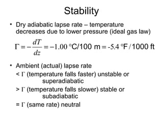
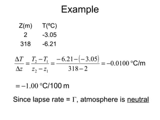
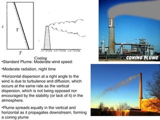
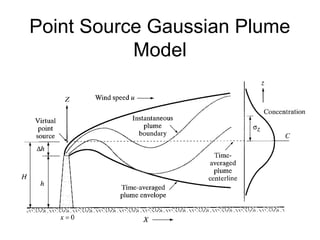
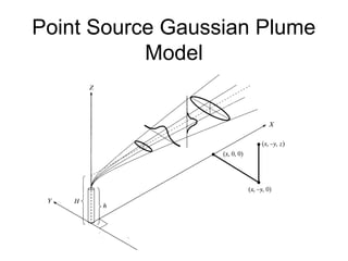
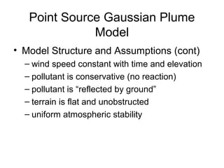
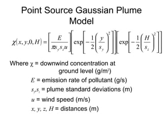
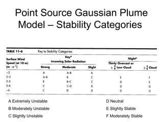
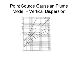
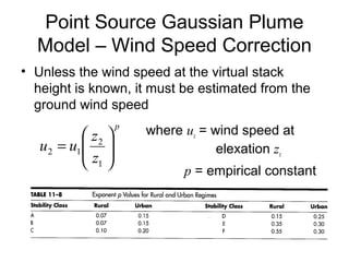
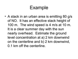
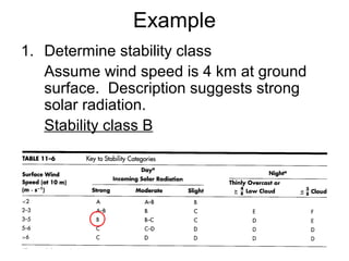
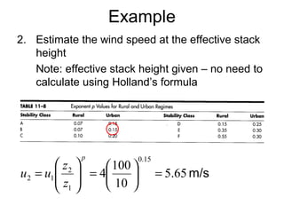
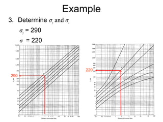
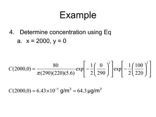
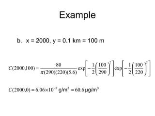
The document discusses meteorological parameters that influence air quality and dispersion modeling. Primary parameters include wind speed, direction, and atmospheric stability, while secondary parameters include temperature, precipitation, and topography. Atmospheric stability is determined by comparing the ambient lapse rate to the dry adiabatic lapse rate. Stability categories include unstable, neutral, and stable atmospheres. Plume rise and dispersion are influenced by stability, with unstable air resulting in greater vertical mixing and stable air suppressing vertical dispersion. The Gaussian plume model is presented as a method to estimate pollutant concentrations downwind of a point source.

1. Meteorology and Dispersion Modeling
Air Quality and Meteorology
• Primary Metrological Parameter
– Wind speed, Wind Direction, Atmospheric Stability
• Secondary Metrological Parameter
– sunlight
– temperature
– precipitation and humidity
– Topography
– Energy from the sun and earth’s rotation drives
atmospheric circulation

2. Stability
• Dry adiabatic lapse rate – temperature
decreases due to lower pressure (ideal gas law)
dT
G = - = -1.00 °C/100 m = -5.4 °F/1000 ft
dz
• Ambient (actual) lapse rate
< Г (temperature falls faster) unstable or
superadiabatic
> Г (temperature falls slower) stable or
subadiabatic
= Г (same rate) neutral

3. Example
Z(m) T(ºC)
2 -3.05
318 -6.21
( ) = - °C/m
-
T T
T
D = -
= - - -
0.0100
2 1
z -
z
D
6.21 3.05
318 2
2 1
z
= -1.00 °C/100 m
Since lapse rate = Г, atmosphere is neutral

4. •Standard Plume: Moderate wind speed:
•Moderate radiation, night time
•Horizontal dispersion at a right angle to the
wind is due to turbulence and diffusion, which
occurs at the same rate as the vertical
dispersion, which is not being opposed nor
encouraged by the stability (or lack of it) in the
atmosphere.
•Plume spreads equally in the vertical and
horizontal as it propagates downstream, forming
a coning plume

5. Example
Z(m) T(ºC)
10 5.11
202 1.09
T T
T
D 0.0209
= - °C/m
= -
1.09 5.11
-
= -
2 1
z -
z
D
202 10
2 1
z
= -2.09 °C/100 m
Since lapse rate is more negative than Г,
(-1.00 ºC/100 m), atmosphere is unstable

6. •In unstable air, the plume will whip up and down as the atmosphere mixes
around (whenever an air parcel goes up, there must be air going down
someplace else to maintain continuity, and the plume follows these air currents).
This gives the plume the appearance that it is looping around.
•Vertical dispersion is very high.
•Less wind speed: Strong & Moderate radiation, day time Mechanical Turbulence
is enhanced.
•High probability of high concentrations sporadically at ground level close to
stack.

7. Example
Z(m) T(ºC)
18 14.03
286 12.56
T T
T
D 0.0055
= - °C/m
= -
12.56 14.03
-
= -
2 1
z -
z
D
286 18
2 1
z
= -0.55 °C/100 m
Suppress Vertical Dispersion
Since lapse rate more positive than Г,
atmosphere is stable

8. •High wind speed: Night time, High horizontal dispersion, Vertical dispersion is
suppresses by stable atmosphere.
•In the vertical, dispersion is suppressed by the stability of the atmosphere, so
pollution does not spread toward the ground. This results in very low pollution
concentrations at the ground

9. Temperature Inversions
• Extreme case of stability when lapse rate
is actually positive, i.e. temperature
increases with altitude
• Resulting temperature inversion prevents
nearly all upward mixing

10. Fanning Plume:
Usually occurs at night, or 1200m-1800m above ground. There is high ground
concentration if stack is short or if plume moves through rugged terrain. Occurs
in stable inversion atmospheric conditions.

11. Lofting Plume: favorable in the sense that fewer impacts
at ground level. Pollutants go up into environment. They
are created when atmospheric conditions are unstable
above the plume

12. Fumigation:
most dangerous plume: contaminants are all coming
down to ground level. They are created when
atmospheric conditions are inversion stable above the
plume and unstable below. This happens most often
after the daylight sun has warmed the atmosphere,
which turns a night time fanning plume into fumigation
for about a half an hour.

13. Effect of Lapse Rate on Plumes

14. Point Source Gaussian Plume
Model

15. Point Source Gaussian Plume
Model

16. Point Source Gaussian Plume
Model
• Model Structure and Assumptions
– pollutants released from a “virtual point
source”
– advective transport by wind
– dispersive transport (spreading) follows
normal (Gaussian) distribution away from
trajectory
– constant emission rate

17. Point Source Gaussian Plume
Model
• Model Structure and Assumptions (cont)
– wind speed constant with time and elevation
– pollutant is conservative (no reaction)
– pollutant is “reflected by ground”
– terrain is flat and unobstructed
– uniform atmospheric stability

18. Point Source Gaussian Plume
Model
x y H E
, ,0, exp 1
( )
ù
é
ù
é
ö
æ
ù
é
=
y
y z y z s
Where χ = downwind concentration at
ground level (g/m3)
é
é
exp 1
E = emission rate of pollutant (g/s)
sy,sz = plume standard deviations (m)
u = wind speed (m/s)
x, y, z, H = distances (m)
ù
ú ú
û
ê ê
ë
ù
ú ú
û
ê ê
ë
ö
÷ ÷ø
æ
ç çè
-
ú ú
û
ê ê ë
ú ú
û
ê ê
ë
÷ ÷
ø
ç ç
è
-
ú úû
ê êë
2 2
2
2
H
s
s s u
p
c

19. Point Source Gaussian Plume
Model – Effective Stack Height
H = h + DH
where
H = Effective stack height (m)
h = height of physical stack (m)
ΔH = plume rise (m)

20. Point Source Gaussian Plume
Model – Effective Stack Height
• Holland’s formula
æ D = + ´ - P T - T
d
( )
é
æ
H v
s 1.5 2.68 10 2 s a
where vs = stack velocity (m/s)
d = stack diameter (m)
u = wind speed (m)
P = pressure (kPa)
Ts = stack temperature (ºK)
Ta = air temperature (ºK)
ù
ú úû
ê êë
ö
÷ ÷ø
ç çè
ö
÷ ÷ø
ç çè
T
u
a

21. Point Source Gaussian Plume
Model – Stability Categories
A Extremely Unstable D Neutral
B Moderately Unstable E Slightly Stable
C Slightly Unstable F Moderately Stable

22. Point Source Gaussian Plume
Model – Horizontal Dispersion

23. Point Source Gaussian Plume
Model – Vertical Dispersion

24. Point Source Gaussian Plume
Model – Wind Speed Correction
• Unless the wind speed at the virtual stack
height is known, it must be estimated from the
ground wind speed
where ux = wind speed at
elexation zx
p = empirical constant
p
æ
u u z ÷ ÷ø
2
z
ö
ç çè
=
1
2 1

25. Example
• A stack in an urban area is emitting 80 g/s
of NO. It has an effective stack height of
100 m. The wind speed is 4 m/s at 10 m.
It is a clear summer day with the sun
nearly overhead. Estimate the ground
level concentration at a) 2 km downwind
on the centerline and b) 2 km downwind,
0.1 km off the centerline.

26. Example
1. Determine stability class
Assume wind speed is 4 km at ground
surface. Description suggests strong
solar radiation.
Stability class B

27. Example
2. Estimate the wind speed at the effective stack
height
Note: effective stack height given – no need to
calculate using Holland’s formula
5.65 m/s
4 100
= æ ÷ ÷ø
u u z
÷ø
= 2 1 10
0.15
2
1
ö çè
ö
ç çè æ
=
p
z

28. Example
3. Determine σy and σz
σy = 290
σz = 220
290
220

29. Example
4. Determine concentration using Eq
a. x = 2000, y = 0
ù
ú úû
é
ê êë
100
2
ö çè
÷ø
- æ
ù
ú úû
é
exp 1
ê êë
0
ö çè
÷ø
(2000,0) 80
= - æ
2 2
220
exp 1
290
2
p
(290)(220)(5.6)
C
C(2000,0) = 6.43´10-5 g/m3 = 64.3 μg/m3

30. Example
b. x = 2000, y = 0.1 km = 100 m
ù
ú úû
é
ê êë
100
2
ö çè
÷ø
- æ
ù
ú úû
é
ê êë
100
2
ö çè
÷ø
(2000,100) 80
= - æ
2 2
220
exp 1
290
exp 1
p
(290)(220)(5.6)
C
C(2000,0) = 6.06´10-5 g/m3 = 60.6 μg/m3