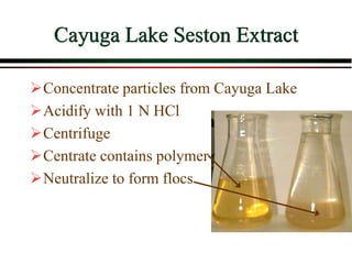
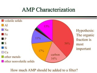
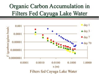
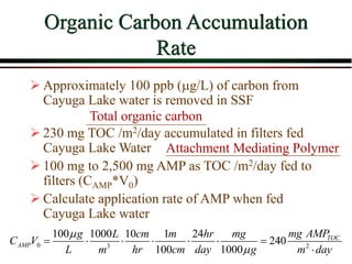
Download to read offline


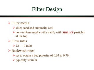
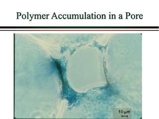
![Overall Filter Performance
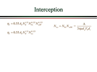
Iwasaki (1937) developed relationships
describing the performance of deep bed
filters.
0
=
dC
C
dz
C is the particle concentration [number/L3]
0 is the initial filter coefficient [1/L]
z is the media depth [L]
The particle’s chances of being caught are the same at all
depths in the filter; pC* is proportional to depth
0
=
dC
dz
C
0
0
0
=
C z
C
dC
dz
C
0
0
ln =
C
z
C
0
0
1
log *
ln 10
C
pC z
C
](https://image.slidesharecdn.com/06filtration-221221090252-66f88678/85/06-Filtration-ppt-6-320.jpg)


The document summarizes information from public health reports on the decline of typhoid fever in the late 19th/early 20th century. It finds that: 1) The decline happened gradually over time and was not associated with any centralized intervention like water filtration or chlorination. 2) Improved personal hygiene was likely the dominant factor in reducing typhoid, as the disease spread through food preparation with contaminated hands rather than centralized systems like water or milk. 3) Other factors like refrigeration and commercial/home refrigeration may have reduced summertime increases in typhoid by limiting bacterial growth in food.