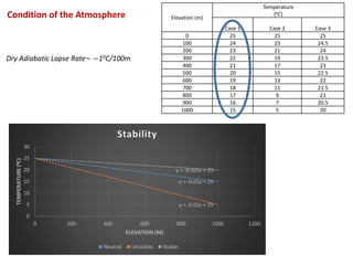
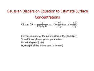
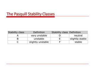
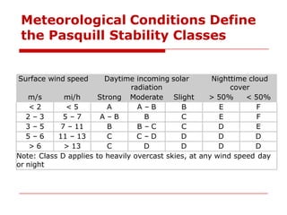
Elevation (m)
Temperature
(0C)
Case 1 Case 2 Case 3
0 25 25 25
100 24 23 24.5
200 23 21 24
300 22 19 23.5
400 21 17 23
500 20 15 22.5
600 19 13 22
700 18 11 21.5
800 17 9 21
900 16 7 20.5
1000 15 5 20
y = -0.01x + 25
y = -0.02x + 25
y = -0.005x + 25
0
5
10
15
20
25
30
0 200 400 600 800 1000 1200
TEMPERATURE
(
0
C)
ELEVATION (M)
Stability
Neutral Unstable Stable
Dry Adiabatic Lapse Rate~ −10C/100m
Condition of the Atmosphere
MODELING
Plume from Stacks
GAUSSIAN DISPERSION
Instantaneous and Time-averaged Plume
 At any given time, the
plume looks rather
turbulent and does not
have a well defined
shape
 However, under steady
wind condition and
averaged over
sufficient time, the
plume shows well
defined shape
Plume photographs (a) instantaneous 1/50s exposure,
(b) 5-min time exposure (Slade, 1968) – Walton J.C. (2008)
Pollutant Concentration Profile
Gaussian Distribution of Pollutant Concentration
 Time-averaged pollutant
concentration follows Gaussian
distribution:
y2
2
: Plume spread
1  
C(y)  exp− 
 2 2

0
Distance away from the center
Pollutant
Concentration
s s
s
s
More about Sy and Sz
 Called “plume spread parameter”
 Function of downwind distance (x)
◼ The further downwind, the greater the
spread parameter values
 Function of atmospheric stability
◼ The more unstable the larger the
parameter values
 Sz usually smaller than Sy
Gaussian Dispersion Equation to Estimate Surface
Concentrations
E= Emission rate of the pollutant from the stack (g/s)
Sy and Sz are plume spread parameters
U= Wind speed (m/s)
He=Height of the plume central line (m)
C x, y, 0 =
E
 SySz U
exp(−
y2
2Sy
2) exp(−
He
2
2Sz
2)
The Pasquill Stability Classes
Stability class Definition Stability class Definition
A very unstable D neutral
B unstable E slightly stable
C slightly unstable F stable
Meteorological Conditions Define
the Pasquill Stability Classes
Surface wind speed Daytime incoming solar
radiation
Nighttime cloud
cover
m/s mi/h Strong Moderate Slight > 50% < 50%
< 2 < 5 A A – B B E F
2 – 3 5 – 7 A – B B C E F
3 – 5 7 – 11 B B – C C D E
5 – 6 11 – 13 C C – D D D D
> 6 > 13 C D D D D
Note: Class D applies to heavily overcast skies, at any wind speed day
or night
Determine Solar Radiation Strength
 As a rule of thumb
◼ Strong: Solar intensity > 700 W/m2
◼ Moderate: Solar intensity > 350 W/m2
◼ Slight: Solar intensity > 100 W/m2
◼ Solar intensity < 100 W/m2 but still day
hours → neutral
Sy, Sz Charts
S
y
Equations to Estimate Sy and Sz
a, c, d, f are parameters. They are functions of stability classes and
distance downwind (x). NOTE: 'x' should be in units of km.
Stability a
x<1km x>1km
c d f c d f
A 213 440.8 1.941 9.27 459.7 2.094 -9.6
B 156 106.6 1.149 3.3 108.2 1.098 2
C 104 61 0.911 0 61 0.911 0
D 68 33.2 0.725 -1.7 44.5 0.516 -13
E 50.5 22.8 0.678 -1.3 55.4 0.305 -34
F 34 14.35 0.74 -0.35 62.6 0.18 -48.6
𝑆𝑧 = 𝑐 × 𝑥𝑑 + 𝑓
𝑆𝑦 = 𝑎 × 𝑥0.894
Example Problem
Given:
• E=127 g/s
• x=850 m
• y=0
• He=101 m
• U=4.5 m/s
• Strong solar radiation
Surface wind speed Daytime incoming solar
radiation
Nighttime cloud
cover
m/s mi/h Strong Moderate Slight > 50% < 50%
< 2 < 5 A A – B B E F
2 – 3 5 – 7 A – B B C E F
3 – 5 7 – 11 B B – C C D E
5 – 6 11 – 13 C C – D D D D
> 6 > 13 C D D D D
Note: Class D applies to heavily overcast skies, at any wind speed day
or night
Step 1
Estimate Plume Spread parameters
C x, y, 0 =
E
 SySz U
exp(−
y2
2Sy
2) exp(−
He
2
2Sz
2)
𝑆𝑦 = 𝑎 × 𝑥0.894
Stability a
x<1km x>1km
c d f c d f
A 213 440.8 1.941 9.27 459.7 2.094 -9.6
B 156 106.6 1.149 3.3 108.2 1.098 2
C 104 61 0.911 0 61 0.911 0
D 68 33.2 0.725 -1.7 44.5 0.516 -13
E 50.5 22.8 0.678 -1.3 55.4 0.305 -34
F 34 14.35 0.74 -0.35 62.6 0.18 -48.6
𝑆𝑦 =134.9 m
𝑆𝑧 = 𝑐 × 𝑥𝑑
+ 𝑓
Sz =91.7 m
Step 2
Estimate Surface Concentration using Gaussian Dispersion Equation
C x, y, 0 =
E
 SySz U
exp(−
y2
2Sy
2) exp(−
He
2
2Sz
2)

4. AQ part3.pdf

  • 1.
    Elevation (m) Temperature (0C) Case 1Case 2 Case 3 0 25 25 25 100 24 23 24.5 200 23 21 24 300 22 19 23.5 400 21 17 23 500 20 15 22.5 600 19 13 22 700 18 11 21.5 800 17 9 21 900 16 7 20.5 1000 15 5 20 y = -0.01x + 25 y = -0.02x + 25 y = -0.005x + 25 0 5 10 15 20 25 30 0 200 400 600 800 1000 1200 TEMPERATURE ( 0 C) ELEVATION (M) Stability Neutral Unstable Stable Dry Adiabatic Lapse Rate~ −10C/100m Condition of the Atmosphere
  • 2.
  • 3.
    Instantaneous and Time-averagedPlume  At any given time, the plume looks rather turbulent and does not have a well defined shape  However, under steady wind condition and averaged over sufficient time, the plume shows well defined shape Plume photographs (a) instantaneous 1/50s exposure, (b) 5-min time exposure (Slade, 1968) – Walton J.C. (2008)
  • 5.
  • 6.
    Gaussian Distribution ofPollutant Concentration  Time-averaged pollutant concentration follows Gaussian distribution: y2 2 : Plume spread 1   C(y)  exp−   2 2  0 Distance away from the center Pollutant Concentration s s s s
  • 7.
    More about Syand Sz  Called “plume spread parameter”  Function of downwind distance (x) ◼ The further downwind, the greater the spread parameter values  Function of atmospheric stability ◼ The more unstable the larger the parameter values  Sz usually smaller than Sy
  • 8.
    Gaussian Dispersion Equationto Estimate Surface Concentrations E= Emission rate of the pollutant from the stack (g/s) Sy and Sz are plume spread parameters U= Wind speed (m/s) He=Height of the plume central line (m) C x, y, 0 = E  SySz U exp(− y2 2Sy 2) exp(− He 2 2Sz 2)
  • 9.
    The Pasquill StabilityClasses Stability class Definition Stability class Definition A very unstable D neutral B unstable E slightly stable C slightly unstable F stable
  • 10.
    Meteorological Conditions Define thePasquill Stability Classes Surface wind speed Daytime incoming solar radiation Nighttime cloud cover m/s mi/h Strong Moderate Slight > 50% < 50% < 2 < 5 A A – B B E F 2 – 3 5 – 7 A – B B C E F 3 – 5 7 – 11 B B – C C D E 5 – 6 11 – 13 C C – D D D D > 6 > 13 C D D D D Note: Class D applies to heavily overcast skies, at any wind speed day or night
  • 11.
    Determine Solar RadiationStrength  As a rule of thumb ◼ Strong: Solar intensity > 700 W/m2 ◼ Moderate: Solar intensity > 350 W/m2 ◼ Slight: Solar intensity > 100 W/m2 ◼ Solar intensity < 100 W/m2 but still day hours → neutral
  • 12.
  • 13.
    Equations to EstimateSy and Sz a, c, d, f are parameters. They are functions of stability classes and distance downwind (x). NOTE: 'x' should be in units of km. Stability a x<1km x>1km c d f c d f A 213 440.8 1.941 9.27 459.7 2.094 -9.6 B 156 106.6 1.149 3.3 108.2 1.098 2 C 104 61 0.911 0 61 0.911 0 D 68 33.2 0.725 -1.7 44.5 0.516 -13 E 50.5 22.8 0.678 -1.3 55.4 0.305 -34 F 34 14.35 0.74 -0.35 62.6 0.18 -48.6 𝑆𝑧 = 𝑐 × 𝑥𝑑 + 𝑓 𝑆𝑦 = 𝑎 × 𝑥0.894
  • 14.
    Example Problem Given: • E=127g/s • x=850 m • y=0 • He=101 m • U=4.5 m/s • Strong solar radiation Surface wind speed Daytime incoming solar radiation Nighttime cloud cover m/s mi/h Strong Moderate Slight > 50% < 50% < 2 < 5 A A – B B E F 2 – 3 5 – 7 A – B B C E F 3 – 5 7 – 11 B B – C C D E 5 – 6 11 – 13 C C – D D D D > 6 > 13 C D D D D Note: Class D applies to heavily overcast skies, at any wind speed day or night Step 1 Estimate Plume Spread parameters C x, y, 0 = E  SySz U exp(− y2 2Sy 2) exp(− He 2 2Sz 2)
  • 15.
    𝑆𝑦 = 𝑎× 𝑥0.894 Stability a x<1km x>1km c d f c d f A 213 440.8 1.941 9.27 459.7 2.094 -9.6 B 156 106.6 1.149 3.3 108.2 1.098 2 C 104 61 0.911 0 61 0.911 0 D 68 33.2 0.725 -1.7 44.5 0.516 -13 E 50.5 22.8 0.678 -1.3 55.4 0.305 -34 F 34 14.35 0.74 -0.35 62.6 0.18 -48.6 𝑆𝑦 =134.9 m 𝑆𝑧 = 𝑐 × 𝑥𝑑 + 𝑓 Sz =91.7 m
  • 16.
    Step 2 Estimate SurfaceConcentration using Gaussian Dispersion Equation C x, y, 0 = E  SySz U exp(− y2 2Sy 2) exp(− He 2 2Sz 2)