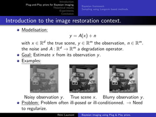
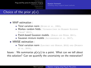
1. The document presents Plug-and-Play priors for Bayesian imaging using Langevin-based sampling methods. 2. It introduces the Bayesian framework for image restoration and discusses challenges in modeling the prior. 3. A Plug-and-Play approach is proposed that uses an implicit prior defined by a denoising network in conjunction with Langevin sampling, termed PnP-ULA. Experiments demonstrate its effectiveness on image deblurring and inpainting tasks.

1. Introduction.
Plug-and-Play priors for Bayesian imaging.
Theoritical results.
Experiments.
Conclusion.
Bayesian imaging using Plug & Play priors.
When Langevin meets Tweedie.
Rémi Laumont
Joint work with:
Valentin De Bortoli, Julie Delon, Andrés Almansa, Alain
Durmus, Marcelo Pereyra.
March 10, 2021
Rémi Laumont Bayesian imaging using Plug & Play priors.

2. Introduction.
Plug-and-Play priors for Bayesian imaging.
Theoritical results.
Experiments.
Conclusion.
1 Introduction.
2 Plug-and-Play priors for Bayesian imaging.
Bayesian framework.
Sampling using Langevin based methods.
3 Theoritical results.
4 Experiments.
A first example on deblurring and inpainting.
Uncertainty Quantification in medical imaging.
5 Conclusion.
Rémi Laumont Bayesian imaging using Plug & Play priors.

3. Introduction.
Plug-and-Play priors for Bayesian imaging.
Theoritical results.
Experiments.
Conclusion.
Bayesian framework.
Sampling using Langevin based methods.
Introduction to the image restoration context.
Modelisation:
y = A(x) + n
with x ∈ Rd the true scene, y ∈ Rm the observation, n ∈ Rm.
the noise and A : Rd → Rm a degradation operator.
Goal: Estimate x from its observation y.
Examples:
Noisy observation y. True scene x. Blurry observation y.
Problem: Problem often ill-posed or ill-conditionned. → Need
to regularize.
Rémi Laumont Bayesian imaging using Plug & Play priors.

4. Introduction.
Plug-and-Play priors for Bayesian imaging.
Theoritical results.
Experiments.
Conclusion.
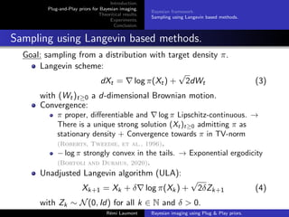
Bayesian framework.
Sampling using Langevin based methods.
Bayesian paradigm.
Bayesian formulation:
p(y|x) ∝ p(x)p(y|x)
where p(x) the prior and p(y|x) is the likelihood (assumed to
be known).
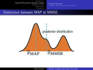
Maximum-A-Posteriori estimator:
x̂MAP =arg max
x∈Rd
p(x|y)=arg min
x∈Rd
{F(x, y) + λR(x)} (1)
where R(x) = − log p(x) and F(x, y) = − log p(y|x).
Minimum Mean Square Error (MMSE) estimator:
x̂MMSE =arg min
u∈Rd
E[kx − uk2
|y] =E[x|y] (2)
Rémi Laumont Bayesian imaging using Plug & Play priors.

5. Introduction.
Plug-and-Play priors for Bayesian imaging.
Theoritical results.
Experiments.
Conclusion.
Bayesian framework.
Sampling using Langevin based methods.
Distinction between MAP et MMSE.
Rémi Laumont Bayesian imaging using Plug & Play priors.

6. Introduction.
Plug-and-Play priors for Bayesian imaging.
Theoritical results.
Experiments.
Conclusion.
Bayesian framework.
Sampling using Langevin based methods.
Choice of the prior p(x).
MAP estimation :
Total variation norm (Rudin et al., 1992).
Markov random fields (“Introduction to Markov Random
Fields” 2011).
Patch-based Gaussian models. (Zoran and Weiss, 2011).
Gaussian mixture models (Aguerrebere et al., 2017).
MMSE estimation :
Total variation norm (Louchet and Moisan, 2013) and (Durmus
et al., 2018).
Issues : We summarize p(x|y) to a point. What can we tell about
this solution? Can we quantify the uncertainty on the restoration?
Rémi Laumont Bayesian imaging using Plug & Play priors.

7. Introduction.
Plug-and-Play priors for Bayesian imaging.
Theoritical results.
Experiments.
Conclusion.
Bayesian framework.
Sampling using Langevin based methods.
Sampling using Langevin based methods.
Goal: sampling from a distribution with target density π.
Langevin scheme:
dXt = ∇ log π(Xt) +
√
2dWt (3)
with (Wt)t≥0 a d-dimensional Brownian motion.
Convergence:
π proper, differentiable and ∇ log π Lipschitz-continuous. →
There is a unique strong solution (Xt)t≥0 admitting π as
stationary density + Convergence towards π in TV-norm
(Roberts, Tweedie, et al., 1996).
− log π strongly convex in the tails. → Exponential ergodicity
(Bortoli and Durmus, 2020).
Unadjusted Langevin algorithm (ULA):
Xk+1 = Xk + δ∇ log π(Xk) +
√
2δZk+1 (4)
with Zk ∼ N(0, Id) for all k ∈ N and δ > 0.
Rémi Laumont Bayesian imaging using Plug & Play priors.

8. Introduction.
Plug-and-Play priors for Bayesian imaging.
Theoritical results.
Experiments.
Conclusion.
Bayesian framework.
Sampling using Langevin based methods.
Role of the discretization step-size δ.
δ controls the trade-off between the convergence speed and
the acuracy of the Markov chain.
1-D example:
π(x) ∝ exp [−x2
/(2σ2
)] with σ = 1.
We sample from πδ ∝ exp [−x2
/(2σ2
δ)] with
σ2
δ = σ2
/(2 − δ/σ2
).
Rémi Laumont Bayesian imaging using Plug & Play priors.

9. Introduction.
Plug-and-Play priors for Bayesian imaging.
Theoritical results.
Experiments.
Conclusion.
Bayesian framework.
Sampling using Langevin based methods.
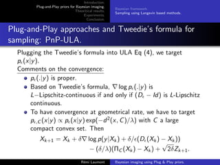
Plug-and-Play approaches.
Targetting p(x|y), Eq (4) becomes
Xk+1 = Xk + δ∇ log p(Xk) + δ∇ log p(y|Xk) +
√
2δZk+1. (5)
Problem: p(x) is unknown and difficult to model. → Implicit prior
such as neural networks to target ∇R e.g (Alain and Bengio,
2014), (Guo et al., 2019),(Romano et al., 2017) and
(Kadkhodaie and Simoncelli, 2021) based on the Tweedie’s
formula :
E[X|X + N = x̃] − x̃ = ∇ log(p ∗ g)(x̃) = ∇ log(p)(x̃), (6)
with X ∼ p, N ∼ N(0, Id) and g a Gaussian kernel (Efron, 2011).
But,
E[X|X + N = x̃] ' D(x̃),
with D a denoiser.
Rémi Laumont Bayesian imaging using Plug Play priors.

10. Introduction.
Plug-and-Play priors for Bayesian imaging.
Theoritical results.
Experiments.
Conclusion.
Bayesian framework.
Sampling using Langevin based methods.
Plug-and-Play approaches and Tweedie’s formula for
sampling: PnP-ULA.
Plugging the Tweedie’s formula into ULA Eq (4), we target
p(x|y).
Comments on the convergence:
p(.|y) is proper.
Based on Tweedie’s formula, ∇ log p(.|y) is
L−Lipschitz-continuous if and only if (D − Id) is L-Lipschitz
continuous.
To have convergence at geometrical rate, we have to target
p,C (x|y) ∝ p(x|y) exp(−d2(x, C)/λ) with C a large
compact convex set. Then
Xk+1 = Xk + δ∇ log p(y|Xk) + δ/(D(Xk) − Xk))
− (δ/λ)(ΠC (Xk) − Xk) +
√
2δZk+1.
Rémi Laumont Bayesian imaging using Plug Play priors.

11. Introduction.
Plug-and-Play priors for Bayesian imaging.
Theoritical results.
Experiments.
Conclusion.
Bayesian framework.
Sampling using Langevin based methods.
PnP-ULA.
1 Require: n ∈ N, y ∈ Rm, , λ, δ 0, C ⊂ Rd convex and
compact.
2 Ensure:
2λ(2Ly + L/) ≤ 1, // Strong convexity in the tails
δ (1/3)(Ly + 1/λ + αL/)−1
. // Stability
3 Initialization: Set X0 = y and k = 0.
4 For k=1, ... N,
5 Zk+1 ∼ N(0, Id).
6 Xk+1 = Xk + δ∇ log(p(y|Xk)) + (δ/)(D(Xk) − Xk) −
(δ/λ)(ΠC (Xk) − Xk) +
√
2δZk+1.
7 End for.
8 return {Xk, k ∈ {0, .., N + 1}}.
Rémi Laumont Bayesian imaging using Plug Play priors.

12. Introduction.
Plug-and-Play priors for Bayesian imaging.
Theoritical results.
Experiments.
Conclusion.
Theorems.
Convergence guarantee under the following assumptions:
The likelihood is C1 and the log-likelihood is
Lipschitz-continuous.
The prior admits a second order moment.
The denoiser residual D is L-Lipschitz.
Estimation of the non-asymptotic error:
|n−1
n
X
k=1
h(Xk) −
Z
Rd
h(x̃)p(x̃|y)dx̃|
≤ {C0β/4
+ C1R−1
C + C2(δ1/2
+ (nδ)−1
)}(1 + E{kX0k4
}). (7)
with h : Rd → R such that supx∈Rd {|h(x)|(1 + kxk2)−1} ≤ 1
Rémi Laumont Bayesian imaging using Plug Play priors.

13. Introduction.
Plug-and-Play priors for Bayesian imaging.
Theoritical results.
Experiments.
Conclusion.
A first example on deblurring and inpainting.
Uncertainty Quantification in medical imaging.
Problem position
-Log-likelihood: F(x, y) = (Ax − y)2/(2σ2) with σ = 1/255.
Deblurring: A encodes a bloc filter of size 9.
Inpainting: A is a diagonal matrix with 1 or 0 on the
diagonal and hidding 80% of the pixels in the original image.
Original images:
Simpson. Cameraman. Traffic.
Rémi Laumont Bayesian imaging using Plug Play priors.

14. Introduction.
Plug-and-Play priors for Bayesian imaging.
Theoritical results.
Experiments.
Conclusion.
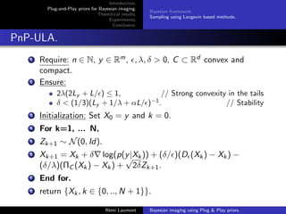
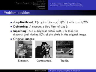
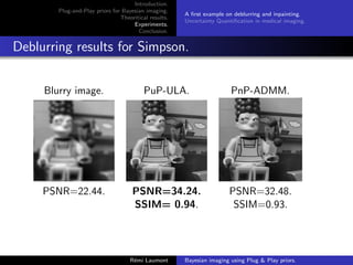
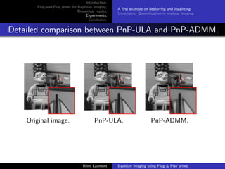
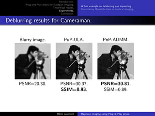
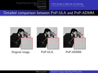
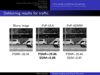
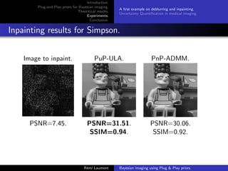
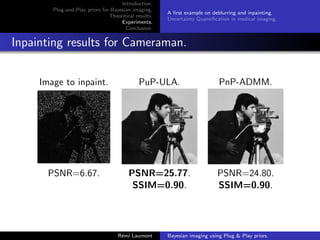
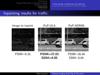
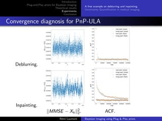
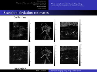
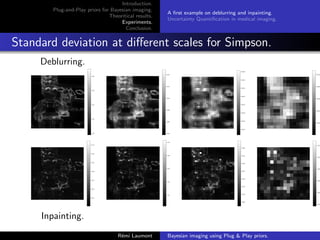
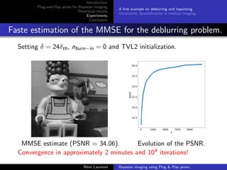
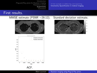
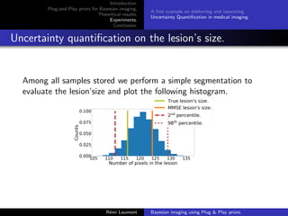
A first example on deblurring and inpainting.
Uncertainty Quantification in medical imaging.
Algorithm parameters
D provided by (Ryu et al., 2019) and such that (D − Id) is
L-Lipschitz with L 1. = (5/255)2.
Comparison with PnP-ADMM with deblurring = (5/255)2 and
inpainting = (40/255)2.
C = [−1, 2]d .
A thinned version of the Markov chain is considered made of
samples stored every 2500 iterations.
n nburn−in δ Initialization
PnP-ULA 2.5e7 2.5e6 3δmax y
Rémi Laumont Bayesian imaging using Plug Play priors.

15. Introduction.
Plug-and-Play priors for Bayesian imaging.
Theoritical results.
Experiments.
Conclusion.
A first example on deblurring and inpainting.
Uncertainty Quantification in medical imaging.
Deblurring results for Simpson.
Blurry image. PuP-ULA. PnP-ADMM.
PSNR=22.44. PSNR=34.24. PSNR=32.48.
SSIM= 0.94. SSIM=0.93.
Rémi Laumont Bayesian imaging using Plug Play priors.

16. Introduction.
Plug-and-Play priors for Bayesian imaging.
Theoritical results.
Experiments.
Conclusion.
A first example on deblurring and inpainting.
Uncertainty Quantification in medical imaging.
Detailed comparison between PnP-ULA and PnP-ADMM.
Original image. PnP-ULA. PnP-ADMM.
Rémi Laumont Bayesian imaging using Plug Play priors.

17. Introduction.
Plug-and-Play priors for Bayesian imaging.
Theoritical results.
Experiments.
Conclusion.
A first example on deblurring and inpainting.
Uncertainty Quantification in medical imaging.
Deblurring results for Cameraman.
Blurry image. PuP-ULA. PnP-ADMM.
PSNR=20.30. PSNR=30.37. PSNR=30.81.
SSIM=0.93. SSIM=0.89.
Rémi Laumont Bayesian imaging using Plug Play priors.

18. Introduction.
Plug-and-Play priors for Bayesian imaging.
Theoritical results.
Experiments.
Conclusion.
A first example on deblurring and inpainting.
Uncertainty Quantification in medical imaging.
Detailed comparison between PnP-ULA and PnP-ADMM.
Original image. PnP-ULA. PnP-ADMM.
Rémi Laumont Bayesian imaging using Plug Play priors.

19. Introduction.
Plug-and-Play priors for Bayesian imaging.
Theoritical results.
Experiments.
Conclusion.
A first example on deblurring and inpainting.
Uncertainty Quantification in medical imaging.
Deblurring results for traffic.
Blurry image PuP-ULA PnP-ADMM
PSNR=20.34. PSNR=29.86. PSNR=29.44.
SSIM=0.89. SSIM=0.87.
Rémi Laumont Bayesian imaging using Plug Play priors.

20. Introduction.
Plug-and-Play priors for Bayesian imaging.
Theoritical results.
Experiments.
Conclusion.
A first example on deblurring and inpainting.
Uncertainty Quantification in medical imaging.
Inpainting results for Simpson.
Image to inpaint. PuP-ULA. PnP-ADMM.
PSNR=7.45. PSNR=31.51. PSNR=30.06.
SSIM=0.94. SSIM=0.92.
Rémi Laumont Bayesian imaging using Plug Play priors.

21. Introduction.
Plug-and-Play priors for Bayesian imaging.
Theoritical results.
Experiments.
Conclusion.
A first example on deblurring and inpainting.
Uncertainty Quantification in medical imaging.
Inpainting results for Cameraman.
Image to inpaint. PuP-ULA. PnP-ADMM.
PSNR=6.67. PSNR=25.77. PSNR=24.80.
SSIM=0.90. SSIM=0.90.
Rémi Laumont Bayesian imaging using Plug Play priors.

22. Introduction.
Plug-and-Play priors for Bayesian imaging.
Theoritical results.
Experiments.
Conclusion.
A first example on deblurring and inpainting.
Uncertainty Quantification in medical imaging.
Inpainting results for traffic.
Image to inpaint. PuP-ULA. PnP-ADMM.
PSNR=8.35. PSNR=27.02. PSNR=26.46.
SSIM=0.85. SSIM=0.84.
Rémi Laumont Bayesian imaging using Plug Play priors.

23. Introduction.
Plug-and-Play priors for Bayesian imaging.
Theoritical results.
Experiments.
Conclusion.
A first example on deblurring and inpainting.
Uncertainty Quantification in medical imaging.
Convergence diagnosis for PnP-ULA
Deblurring.
Inpainting.
kMMSE − Xkk2
2. ACF.
Rémi Laumont Bayesian imaging using Plug Play priors.

24. Introduction.
Plug-and-Play priors for Bayesian imaging.
Theoritical results.
Experiments.
Conclusion.
A first example on deblurring and inpainting.
Uncertainty Quantification in medical imaging.
Standard deviation estimates.
Deblurring.
Inpainting.
Rémi Laumont Bayesian imaging using Plug Play priors.

25. Introduction.
Plug-and-Play priors for Bayesian imaging.
Theoritical results.
Experiments.
Conclusion.
A first example on deblurring and inpainting.
Uncertainty Quantification in medical imaging.
Standard deviation at different scales for Simpson.
Deblurring.
Inpainting.
Rémi Laumont Bayesian imaging using Plug Play priors.

26. Introduction.
Plug-and-Play priors for Bayesian imaging.
Theoritical results.
Experiments.
Conclusion.
A first example on deblurring and inpainting.
Uncertainty Quantification in medical imaging.
Animation
To show.
Rémi Laumont Bayesian imaging using Plug Play priors.

27. Introduction.
Plug-and-Play priors for Bayesian imaging.
Theoritical results.
Experiments.
Conclusion.
A first example on deblurring and inpainting.
Uncertainty Quantification in medical imaging.
First conclusions.
3 Computation of higher moments.
3 First uncertainty study.
3 Convergence Diagnosis.
7 It is time-and memory-consuming (' 65 computation hours
on Titan XP).
→ it depends on our goals.
Rémi Laumont Bayesian imaging using Plug Play priors.

28. Introduction.
Plug-and-Play priors for Bayesian imaging.
Theoritical results.
Experiments.
Conclusion.
A first example on deblurring and inpainting.
Uncertainty Quantification in medical imaging.
Faste estimation of the MMSE for the deblurring problem.
Setting δ = 24δth, nburn−in = 0 and TVL2 initialization.
MMSE estimate (PSNR = 34.06). Evolution of the PSNR.
Convergence in approximately 2 minutes and 104 iterations!
Rémi Laumont Bayesian imaging using Plug Play priors.

29. Introduction.
Plug-and-Play priors for Bayesian imaging.
Theoritical results.
Experiments.
Conclusion.
A first example on deblurring and inpainting.
Uncertainty Quantification in medical imaging.
Faste estimation of the MMSE for the inpainting problem.
Setting δ = 24δth, nburn−in = 0 and TVL2 initialization.
MMSE estimate (PSNR = 30.78). Evolution of the PSNR.
Results obtained after 1.5 × 105 iterations and 20 minutes.
Rémi Laumont Bayesian imaging using Plug Play priors.

30. Introduction.
Plug-and-Play priors for Bayesian imaging.
Theoritical results.
Experiments.
Conclusion.
A first example on deblurring and inpainting.
Uncertainty Quantification in medical imaging.
Problem position and parameter presentation.
The original image x is a Computed Tomography slice from
(Yan et al., 2018) with an annotated lesion.
-Log-likelihood: F(x, y) = (x − y)2/(2σ2) with σ = 25/255.
We set n = 5 × 106 with nburn−in = 5 × 104, init = y.
We consider a thinned Markov chain made of samples stored
every 500 iterations.
Original image from (Yan et al., 2018). Noisy image (PSNR = 20.17).
Rémi Laumont Bayesian imaging using Plug Play priors.

31. Introduction.
Plug-and-Play priors for Bayesian imaging.
Theoritical results.
Experiments.
Conclusion.
A first example on deblurring and inpainting.
Uncertainty Quantification in medical imaging.
First results.
MMSE estimate (PSNR =29.12). Standard deviation estimate.
ACF.
Rémi Laumont Bayesian imaging using Plug Play priors.

32. Introduction.
Plug-and-Play priors for Bayesian imaging.
Theoritical results.
Experiments.
Conclusion.
A first example on deblurring and inpainting.
Uncertainty Quantification in medical imaging.
Uncertainty quantification on the lesion’s size.
Among all samples stored we perform a simple segmentation to
evaluate the lesion’size and plot the following histogram.
Rémi Laumont Bayesian imaging using Plug Play priors.

33. Introduction.
Plug-and-Play priors for Bayesian imaging.
Theoritical results.
Experiments.
Conclusion.
Conclusion.
Summary.
Development of a Langevin based algorithm with detailed
convergence guarantees under realistic hypothesis.
Estimation of the non-asymptotic error when using this
algorithm.
Efficient methods on different classical inverse problems.
Future work.
Develop accelerated computation algorithms using this
framework (Pereyra et al., 2020).
Apply this framework to uncertainty quantification in
astrophysics or medical imaging.
Rémi Laumont Bayesian imaging using Plug Play priors.

34. Introduction.
Plug-and-Play priors for Bayesian imaging.
Theoritical results.
Experiments.
Conclusion.
If you want to know more you can:
1 ask questions.
2 visit this website https://arxiv.org/abs/2103.04715.
Rémi Laumont Bayesian imaging using Plug Play priors.

35. References
Aguerrebere, Cecilia, Andres Almansa, Julie Delon, Yann Gousseau, and Pablo Muse
(2017). “A Bayesian Hyperprior Approach for Joint Image Denoising and
Interpolation, With an Application to HDR Imaging”. In: IEEE Transactions on
Computational Imaging 3.4, pp. 633–646. issn: 2333-9403. doi:
10.1109/TCI.2017.2704439. arXiv: 1706.03261 (cit. on p. 6).
Alain, Guillaume and Yoshua Bengio (2014). “What Regularized Auto-Encoders Learn
from the Data-Generating Distribution”. In: Journal of Machine Learning Research
15, pp. 3743–3773. issn: 1532-4435. arXiv: 1211.4246 (cit. on p. 9).
Bortoli, Valentin De and Alain Durmus (2020). Convergence of diffusions and their
discretizations: from continuous to discrete processes and back. arXiv: 1904.09808
[math.PR] (cit. on p. 7).
Durmus, Alain, Eric Moulines, and Marcelo Pereyra (2018). “Efficient bayesian
computation by proximal markov chain monte carlo: when langevin meets moreau”.
In: SIAM Journal on Imaging Sciences 11.1, pp. 473–506 (cit. on p. 6).
Efron, Bradley (2011). “Tweedie’s Formula and Selection Bias”. In: Journal of the
American Statistical Association 106.496, pp. 1602–1614. issn: 0162-1459. doi:
10.1198/jasa.2011.tm11181 (cit. on p. 9).
Guo, Bichuan, Yuxing Han, and Jiangtao Wen (2019). “AGEM : Solving Linear
Inverse Problems via Deep Priors and Sampling”. In: (NeurIPS) Advances in Neural
Rémi Laumont Bayesian imaging using Plug Play priors.

36. References
Information Processing Systems. Ed. by Curran Associates Inc., pp. 545–556
(cit. on p. 9).
“Introduction to Markov Random Fields” (2011). In: Markov Random Fields for Vision
and Image Processing. The MIT Press. doi: 10.7551/mitpress/8579.003.0001
(cit. on p. 6).
Kadkhodaie, Zahra and Eero P. Simoncelli (2021). Solving Linear Inverse Problems
Using the Prior Implicit in a Denoiser. arXiv: 2007.13640 [cs.CV] (cit. on p. 9).
Louchet, Cécile and Lionel Moisan (2013). “Posterior expectation of the total variation
model: Properties and experiments”. In: SIAM Journal on Imaging Sciences 6.4,
pp. 2640–2684. issn: 19364954. doi: 10.1137/120902276 (cit. on p. 6).
Pereyra, Marcelo, Luis Vargas Mieles, and Konstantinos C. Zygalakis (2020).
“Accelerating proximal Markov chain Monte Carlo by using an explicit stabilized
method”. In: SIAM J. Imaging Sci. 13.2, pp. 905–935. doi: 10.1137/19M1283719
(cit. on p. 33).
Roberts, Gareth O, Richard L Tweedie, et al. (1996). “Exponential convergence of
Langevin distributions and their discrete approximations”. In: Bernoulli 2.4,
pp. 341–363 (cit. on p. 7).
Romano, Yaniv, Michael Elad, and Peyman Milanfar (2017). “The Little Engine That
Could: Regularization by Denoising (RED)”. In: SIAM Journal on Imaging Sciences
Rémi Laumont Bayesian imaging using Plug Play priors.

37. References
10.4, pp. 1804–1844. issn: 1936-4954. doi: 10.1137/16M1102884. arXiv:
1611.02862 (cit. on p. 9).
Rudin, Leonid I., Stanley Osher, and Emad Fatemi (1992). “Nonlinear total variation
based noise removal algorithms”. In: Physica D: Nonlinear Phenomena 60.1-4,
pp. 259–268. issn: 01672789. doi: 10.1016/0167-2789(92)90242-F (cit. on p. 6).
Ryu, Ernest K., Jialin Liu, Sicheng Wang, Xiaohan Chen, Zhangyang Wang, and
Wotao Yin (2019). “Plug-and-Play Methods Provably Converge with Properly
Trained Denoisers”. In: ICML. arXiv: 1905.05406 (cit. on p. 14).
Yan, Ke, Xiaosong Wang, Le Lu, and Ronald M Summers (2018). “DeepLesion:
automated mining of large-scale lesion annotations and universal lesion detection
with deep learning”. In: Journal of Medical Imaging 5.3, p. 036501 (cit. on p. 30).
Zoran, Daniel and Yair Weiss (2011). “From learning models of natural image patches
to whole image restoration”. In: (ICCV) International Conference on Computer
Vision. IEEE, pp. 479–486. isbn: 978-1-4577-1102-2. doi:
10.1109/ICCV.2011.6126278 (cit. on p. 6).
Rémi Laumont Bayesian imaging using Plug Play priors.