The document introduces the concept of generalized quasi-nonexpansive (GQN) maps. Some key results are: 1) GQN maps generalize quasi-nonexpansive maps but the fixed point set may not always be closed or convex. 2) If a subset satisfies certain conditions, it is a GQN-retract of the space. 3) Under these conditions, the class of GQN-retracts is closed under intersection and the common fixed point set of an increasing sequence of GQN maps is a GQN-retract.

1. IOSR Journal of Mathematics (IOSR-JM)
e-ISSN: 2278-5728, p-ISSN: 2319-765X. Volume 11, Issue 1 Ver. III (Jan - Feb. 2015), PP 33-36
www.iosrjournals.org
DOI: 10.9790/5728-11133336 www.iosrjournals.org 33 |Page
A Generalization of QN-Maps
S. C. Arora1
, Vagisha Sharma2
1
Former Professor& Head, Department of Mathematics, University of Delhi, Delhi, INDIA
2
Department of Mathematics, IP College for Women, (University of Delhi), Delhi, INDIA
Abstract: The notion of GQN-Maps is introduced and some results regarding these maps are obtained.
Keywords: Quasi-nonexpansive maps, GQN-maps, convex set, fixed point set, continuous maps, retract,
retraction mapping, locally weakly compact, conditional fixed point property.
AMS subject classification codes: 47H10, 54H25
I. Introduction
A self mapping T of a subset C of a normed linear space X is said to be nonexpansive if Tx – Ty ≤
x – y for allx , y in C [3]. It is quasi- nonexpansiveif T has at least one fixed point p of T in C and Tx – p
≤ x – p for allx in C and for each fixed point p of T in C [5,6].Many results have been proved for
nonexpansive and quasi-nonexpansive mappings. One may referBrowder and Petryshyn [1], Bruck [4],
Chidume [5], Das and Debata [6], Dotson [7],Petryshyn and Williamson [8], Rhoades [9], Singh and Nelson
[11], Senter and Dotson [10]and many more.
The purpose of the present paper is to introduce the notion of generalized quasi-nonexpansive
mappings (GQN-maps).
Throughout the paper, unless stated otherwise, X denotes a Banach space, , the field of real numbers,
A, the closure of A and F(T), the fixed point set of a mapping T. A subset C of X is locally compact if each point
of C has a compact neighbourhood in C [12]. The mapping r from a set C onto A, A being a subset of C, is a
retraction mapping if ra = afor alla in A[2].
II. Definition
2.1:A selfmapping T of a subset C of X is said to be generalised quasi-nonexpansive mapping (GQN-map)
provided T has at least one fixed point and corresponding to each fixed point T, there exists a constant M
depending on the fixed point p (referred as M(p)) in  such that for each x belonging to C,
Tx – p ≤ M(p) x – p 
Clearly, every quasi-nonexpansive map is a GQN map. However, the converse may not be true.
Example 1.2 establishes the same. It is well known that for a linear map, the fixed point setF(T) is convex and
for a continuous map, the fixed point set is closed. But there are non-linear discontinuous GQN-maps whose
fixed point sets are closed and convex.
Example 2.2:
(i) Define T:[0,
π
2
]→ [0,
π
2
] by
Tx = x + ( x −
π
4
)( cosx + 1)
Then F(T) = {
π
4
}
(ii) Define T: [0,1]→ [0,1] by
Tx= n + 1 x − 1 ,
1
n+1
< x ≤
1
n
, n = 1,2, . . ..
T(0) = 1
Then F(T) = {1,
1
2
,
1
3
,
1
4
, ........}
(iii) Define T:  +
→ +
by
Tx =
1−x
n
,
1
n+1
< x ≤
1
n
, n = 0,1,2,3, . . . . ..
Then F(T) = {
1
n+1
: n = 0,1,2,3,.....}
(iv) Consider the Banach space n
= {(x1, x2, x3 … . xn): xifor all i = 1,2,3,. . . . . . n}.
Set C = {(x1, x2, x3 … . xn):xn = 0for all n > 2,x2 ≠ 0, x2 ≠1}.

2. A Generalization of QN-Maps
DOI: 10.9790/5728-11133336 www.iosrjournals.org 34 |Page
Define T : C → C by
T(x1, x2, 0, 0 … .0) = (2x2 − x2 − 1 x1, x2, 0, 0, … .0)
Then F(T) = {(2, x2, 0,0, . . . ,0): x2 ~{0,1}}.
The above examples show that F(T) may or may not be closed and convex for a GQN-map. Note that except in
example (i), the GQN-maps are discontinuous also. The exact set of conditions under which the fixed point set
of a GQN-map is closed and convex, areyet to obtained, but the conditions for F(T) to be a GQN-retract are
obtained in the next section.
III. Main results
IV.
In this section, C always denotes a closed, bounded and convex subset of the space X.
Definition3.1:A subset A of C is said to be a GQN-retract of C if there exists a retraction mapping r from C
onto A which is a GQN-map.
To find the set of conditions for any nonempty subset of a locally weakly compact set to be aGQN-retract, we
prove the following two lemmas:
Lemma3.2: Suppose A is a nonempty subset of a locally weakly compact set C and let
G(A) = {f: C → C is a GQN-map and f(x) = x for each x in A}. Then G(A) is compact in the topology of
weak-pointwise convergence.
Proof: Fix x0A. For each f G(A), there exists a real number Mf(x0) such that
f(x) – f (x0) ≤ Mf(x0)x – x0for allxC.
Let M x0 = Mff∈G A
Sup
(x0).
Case (i): Let M x0 be finite. For each xC, define Ax= {yC: y – x0≤ M(x0)x – x0}. Then Ax contains
f(x) for each x in C and f in G(A) which gives that G(A) is a subset of the Cartesian product P =x∈C Ax. Now
Ax is convex and weakly compact. So if Axis given the weak topology and P is given the product topology, by
Tychonoff’s theorem for the product of compact sets, P is compact.
Case (ii): Let M x0 be infinite. Then P = C and hence P is compact.
Now to show that G(A) is closed in P, let f be a limit point of G(A) in Pand <f>, a net in G(A) such that f →f.
Then, using lower semi-continuity of the norm function and the fact that f is in G(A), we get that G(A) is a
closed subset of the compact set P and hence is compact as desired.
Lemma3.3: Suppose A is nonempty subset of C and C is locally weakly compact. Then there exists an r in G(A)
such that for each f G(A) we have rx – ry ≤ f x – f(y)  for all x, yin C.
Proof: Define an order < on G(A) by setting f < 𝑔 if f(x) – f(y) ≤g(x) – g(y)  for each x, y in C with
inequality holding for at least one pair of x and y. Also f ≤ g means either f < 𝑔or f = g. Clearly ≤ is a partial
order on G(A).For each f in G(A), we define the initial segmentIs(f) = { gG(A): g ≤ f}. Then, as shown in
lemma 2.2, Is(f) is closed and compact in G(A). Now consider a chain in G(A). Then T = {Is(f): f } is a
chain of compact sets under set- inclusion as a partial order relation.By the finite intersection property for
compact sets, T is bounded below, say, by Is(h). Thenf ≤ h ∀ f  G(A).
Now we prove the desired result in the following form:
Theorem3.4: Suppose C is locally weakly compact and A is a nonempty subset of C. Suppose further that for
each z in C, there exists an h ∈ G(A) such that h(z) A. Then A is a GQN-retract of C.
Proof: By lemma 2.3, there exists an r  G(A) such that for each x, y in C and f G(A)
r(x) – r(y) ≤f(x) – f(y) ...................................................................... (2.1)
Also, it can be easily verified that for each f  G(A), the composite map f ∘ r  G(A).
Since r G(A), it is sufficient to show that for each x  C, r(x)  A. For this, let x  C and put z = r(x).
Then as z C, the hypothesis assures the existence of an h  G(A) such that h(r(x))  A. Now, let h(r(x)) =
y then as h ∘ r  G(A), the inequality 2.1 implies

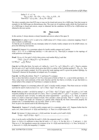
3. A Generalization of QN-Maps
DOI: 10.9790/5728-11133336 www.iosrjournals.org 35 |Page
r(x) – r(y) ≤ h ∘ r (x) – h ∘ r (y) ....................................................................... (2.2)
Since y = h(r(x)) A and r  G(A), therefore, r(y) = y which further implies h(r(y)) = h(y) = y =
h(r(x)). So we get , in view of 2.2, that r(x)  A.
Since for a GQN-map T, the fixed point set F(T) is always nonempty, so we have the following :
Corollary 3.5: Let C be a locally weakly compact set and T: C → C is a GQN-map. Suppose that for each z  C
there exists an h in G(F(T)) such that h(z)  F(T). Then F T is a GQN-retract of C.
Theorem 3.6: Under the conditions of Theorem 2.4, the class of GQN-retracts is closed under arbitrary
intersection.
Proof:By theorem 2.4, the collection { Is(f): f}, where  is a chain in G(A), has a minimal element f in G(A)
which is a GQN-retract of C. Let  = {Af  C: f  G(A) and Af is the corresponding GQN-retract of C}. Clearly
≠ φas A . Order  by AfAgiff ≤ g f and g in G(A). By Zorn’s lemma,  has a minimal element, say,
Ag. It can be seen that g is minimal in G(A).
Put F = Af.f∈G(A) AsA  F(f) for every f, therefore, F is nonempty. Also minimality of g in G(A) implies that
Agis contained in each GQN-retract of C and hence in F. Then F= Ag. Thus F is a GQN-retract of C.
We now establish that the set of common fixed points of an increasing sequence of GQN-maps is a GQN-retract
of C .
Theorem 3.7: Let C be a locally weakly compact subset of X. If <rn> is a sequence of GQN-maps in G(A) such
that the corresponding GQN-retracts F(rn) form an increasing sequence with F(n rn ) ≠ φ then there exists a
GQN-map r from C to C such that F(r) = F(n rn ).
Proof: Consider  = {F(rn): rn is a GQN-retraction of C onto F(rn)}.Order as A ≤ B if A  B. By Zorn’s
lemma, there exists a minimal element, say, F.ThenF= F(n rn). Thus F(n rn ) is a GQN-retract of C.
By hypothesis, F(n rn) ≠ φ. So let  F(n rn). Then pF(rn) for each n. Choose a sequence <n > of
positive numbers such that nn = 1 and let r = nn rn.For each p  F(n rn) and x C,
r(x) – r(p) ≤  ( nn rn ) (x)( nn rn)(p)
≤ nn rn x − rn p 
≤ M(p)x  p
as nn = 1 and M(p) = maxn{Mrn
(p):Mrn
(p) is a constant corresponding to the GQN-map rn}. Thus r is a
GQN-map. Further, using nn = 1, it can be shown that F(r) = F(n rn) which proves the result.
Definition3.8: [3]:A mapping T: C →X is said to satisfy the conditional fixed point property (CFPP) if either T
has no fixed point or T has a fixed point in each nonempty bounded closed set it leaves invariant.
Definition 3.9: A nonempty subset C is said to have the hereditary fixed point property (HFPP) for GQN maps
if every nonempty bounded closed convex subset of C has a fixed point for GQN- mappings.
Following Bruck [3], we prove the following:
Theorem 3.10: If C is locally weakly compact and T: C →C is a GQN-map which satisfies CFPP then F(T) is a
GQN retract of C.
Proof: By definition of T, F(T) is nonempty. For a fixed z in C, define K = {f(z) ∶ f  G(F(T))}. In view of the
compactness of G(F(T)), following [3], K is weakly compact and hence bounded. Also, K . For f and g in
G(F(T) and 0 ≤  ≤ 1, consider f + (1 − )g. If y0 F(T) then F(y0) = y0= g(y0) so that for all x, y in C,
(f + (1 )g)(x)y0  ≤ (Mf (y0)+ (1 )Mg (y0)xx0 
where Mf (y0 ) andMg (y0 ) are real numbers corresponding to the fixed point y0 and for mappings f and g
respectively. Let us putM(Mf + (1)Mg)
(y0) = Mf (y0) + (1 )Mg (y0) then f + (1 )gis a GQN-map.
Also every fixed point x of T is a fixed point of f + (1 )g and hence K is convex. Also for fG(F(T)),
T ∘ f  G(F(T)) i.e. T(K)  K. Therefore, by hypothesis T has a fixed point in K i.e. ∃f G(F(T)) such that
f(z)  F(T) for each z C. Thus, by theorem 2.4, F(T) is a GQN-retract of C.
Corollary3.11: Suppose T: C →C is a GQN-map satisfying CFPP and the convex closure conv(T C ) of the
range of T is locally weakly compact then F(T) is a GQN-retract of C.

4. A Generalization of QN-Maps
DOI: 10.9790/5728-11133336 www.iosrjournals.org 36 |Page
The following result can be proved following the arguments of Bruck [3].
Theorem3.12: Let C be locally weakly compact and {Fα: } be a family of weakly closed GQN retracts of C.
Then
(a) If this family is directed by, then Fαα is a generalised quasi-nonexpansive retract of C.
(b) If each Fα is convex and the family is directed by  then ( Fαα ), the closure of( Fαα ), is a generalised
quasi-nonexpansive retract of C.
Lemma3.13: Let C be weakly compact and satisfies HFPP for GQN-maps. Let F be nonempty GQN- retract of
C and T: C → C is a GQN-map which leaves F invariant. Then F(T) ∩F is a nonempty GQN-retract of C.
Theorem3.14: Suppose C is weakly compact and has HFPP for GQN-maps. If {Tj : 1 ≤ j ≤ n} is a finite family
of commuting GQN-mapsTj: C → C then F(Tj)n
j=1 is a nonempty GQN-retract of C.
Theorem 3.15: Let {Tα: } is a family of GQN-maps of C, where,  is some index set. If exactly one map,
sayTα, of the family is linear and continuous and commutes with each of the remaining then F( Tα ) ∩
( conv. F(Tβ)β≠α ) is nonempty.
Proof: Without loss of generality, we may assume that T1 is linear and continuous such that T1Tα= TαT1 for
allα. Clearly conv (F T1 ) = F(T1). Also for each α, conv (F Tα ) is a nonempty compact convex subset
of C. Linearity and continuity of T1 implies T1(conv (F Tα )conv (F Tα ). So, by Tychonoff’s theorems for
fixed points, T1 has fixed points in conv (F Tα ) and hence the result.
Remark3.16: In the proof of the above result, the condition of the self mapping being GQN-map is required to
assume that F(Tα)’s are nonempty. So if the hypothesis of the theorem contains the fact that F(Tα) ≠ for
allα, the result remains true for an ordinary family of mappings with exactly one map of the family being
linear and continuous.
The result of theorem 2.15 can be extended to a countable intersection of convex closures of F(Ti)’s but the least
conditions required are yet to be traced though the result is trivially true for the family of linear and continuous
maps.
References
[1]. Browder, F.E. andPetryshyn, W.V.: The Solutions Of Iterations Of Nonlinear Functional Analysis Of Banach Spaces, Bull. Amer.
Math. Soc. 72 (1966), 571 – 575.
[2]. Bruck R. E.: Nonexpansive Retracts of Banachspaces, Bull. Amer. Math. Soc. 76 (1970), 384 – 386.
[3]. Bruck, R. E.: Properties of Fixed Points of Nonexpansive Mappings InBanach Spaces, Trans. Amer. Math. Soc., Vol. 179 (1973),
251 – 262.
[4]. Bruck,R.E.: A Common Fixed Point Theorem For A Commuting Family of Nonexpansivemaps, Pac. J. Math., Vol. 53, No.1, 1974,
59 – 71.
[5]. Chidume, C.E.: Quasi-Nonexpansive Mappings AndUniform Asymptotic Regularity, Kobe J. Math. 3 (1986), No.1,29 – 35.
[6]. Das, G. andDebata, J. P.:FixedPoints Of Quasi-Nonexpansive Mappings, Indianj. Pure Appl. Math, 17 (1986), No.11, 1263 – 1269.
[7]. Dotson, W. G.: Fixed Points OfQuasi- Nonexpansive Mappings, J. Australian Math. Soc.13 (1972), 167 – 170.
[8]. Petryshyn, W. V. AND Williamson, T. E.: Strong And Weak Convergence Of The Sequence Of Successive Approximations For
Quasi-Nonexpansive Mapping, J. Math. Anal.Appl. Vol. 43 (1973), 459 – 497.
[9]. Rhoades, B. E.:Fixedpoint Iterations OfGeneralised Nonexpansive Mappings, J. Math. Anal.Appl. Vol. 130 (1988), No. 2, 564 –
576.
[10]. Senter, H. F. And Dotson, W. G.: Approximating Fixed Points OfNonexpansive Mappings, Proc. Amer. Math. Soc. 44 (1974), 375
– 380.
[11]. Singh, K. L. AND Nelson, James L.: Nonstationary Process ForQuasi- Nonexpansivemappings, Math. Japon. 30 (1985), No. 6, 963
– 970.
[12]. Yosida,K.:Functional Analysis, Narosa Publishing House, New Delhi, 1979.