Download as PDF, PPTX
![Introduction: Euclidean Smallest Enclosing Balls
Given d-dimensional P = {p1, ..., pn}, find the “smallest”
(with respect to the volume ≡ radius ≡ inclusion)
ball B = Ball(c, r ) fully covering P:
c∗ = min
c∈Rd
n
max
i=1 kc − pik.
◮ unique Euclidean circumcenter c∗, SEB [19].
◮ optimization problem non-differentiable [10]
c∗ lie on the farthest Voronoi diagram
c
2013-14 Frank Nielsen, ´E
cole Polytechnique & Sony Computer Science Laboratories 2/39](https://image.slidesharecdn.com/smallestenclosingriemannianball-141003080411-phpapp02/85/On-approximating-the-Riemannian-1-center-2-320.jpg)
![Euclidean smallest enclosing balls (SEBs)
◮ 1857: d = 2, Smallest Enclosing Ball? of P = {p1, ..., pn}
(Sylvester [16])
◮ Randomized expected linear time algorithm [19, 5] in fixed
dimension (but hidden constant exponential in d)
◮ Core-set [3] approximation: (1 + ǫ)-approximation in
O( dn
ǫ + 1
ǫ2 )-time in arbitrary dimension, O( dn
ǫ4.5 log 1
ǫ ) [7]
◮ Many other algorithms and heuristics [14, 9, 17], etc.
SEB also known as Minimum Enclosing Ball (MEB), minimax
center, 1-center, bounding (hyper)sphere, etc.
→ Applications in computer graphics (collision detection with ball
cover proxies [15]), in machine learning (Core Vector
Machines [18]), etc.
c
2013-14 Frank Nielsen, ´E
cole Polytechnique & Sony Computer Science Laboratories 3/39](https://image.slidesharecdn.com/smallestenclosingriemannianball-141003080411-phpapp02/85/On-approximating-the-Riemannian-1-center-3-320.jpg)
![Optimization and core-sets [3]
Let c(P) denote the circumcenter of the SEB and r (P) its radius
Given ǫ > 0, ǫ-core-set C ⊂ P, such that
P ⊆ Ball(c(C), (1 + ǫ)r (C))
⇔ Expanding SEB(C) by 1 + ǫ fully covers P
Core-set of optimal size ⌈1
ǫ ⌉, independent of the dimension d,
and n. Note that combinatorial basis for SEB is from 2 to
d + 1 [19].
→ Core-sets find many applications for problems in
large-dimensions.
c
2013-14 Frank Nielsen, ´E
cole Polytechnique & Sony Computer Science Laboratories 4/39](https://image.slidesharecdn.com/smallestenclosingriemannianball-141003080411-phpapp02/85/On-approximating-the-Riemannian-1-center-4-320.jpg)
![Euclidean SEBs from core-sets [2]
B˘adoiu-Clarkson algorithm based on core-sets [2, 3]:
BCA:
◮ Initialize the center c1 ∈ P = {p1, ..., pn}, and
◮ Iteratively update the current center using the rule
ci+1 ← ci +
fi − ci
i + 1
where fi denotes the farthest point of P to ci :
fi = ps , s = argmaxnj
=1kci − pjk
⇒ gradient-descent method
⇒ (1 + ǫ)-approximation after ⌈ 1
ǫ2 ⌉ iterations: O( dn
ǫ2 ) time
⇒ Core-set: f1, ..., fl with l = ⌈ 1
ǫ2 ⌉
c
2013-14 Frank Nielsen, ´E
cole Polytechnique & Sony Computer Science Laboratories 5/39](https://image.slidesharecdn.com/smallestenclosingriemannianball-141003080411-phpapp02/85/On-approximating-the-Riemannian-1-center-5-320.jpg)
![Euclidean SEBs from core-sets: Rewriting with #
a#tb: point (1 − t)a + tb = a + t(b − a) on the line segment [ab].
D(x, y) = kx − yk2, D(x, P) = miny∈P D(x, y)
Algorithm 1: BCA(P, l ).
c1 ← choose randomly a point in P;
for i = 2 to l − 1 do
nj
// farthest point from ci
si ← argmax=1D(ci , pj );
// update the center: walk on the segment [ci , psi ]
ci+1 ← ci# 1
psi ;
i+1
end
// Return the SEB approximation
return Ball(cl , r 2
l = D(cl ,P)) ;
⇒ (1 + ǫ)-approximation after l = ⌈ 1
ǫ2 ⌉ iterations.
c
2013-14 Frank Nielsen, ´E
cole Polytechnique & Sony Computer Science Laboratories 6/39](https://image.slidesharecdn.com/smallestenclosingriemannianball-141003080411-phpapp02/85/On-approximating-the-Riemannian-1-center-6-320.jpg)
![Bregman divergences (incl. squared Euclidean distance)
SEB extended to Bregman divergences BF (· : ·) [13]
BF (c : x) = F(c) − F(x) − hc − x,∇F(x)i,
BF (c : X) = minx∈X BF (c : x)
F
ˆp
ˆq
q p
Hq
H′
q
BF (p, q) = Hq − H′
q
⇒ Bregman divergence = remainder of a first order Taylor
expansion.
c
2013-14 Frank Nielsen, ´E
cole Polytechnique & Sony Computer Science Laboratories 7/39](https://image.slidesharecdn.com/smallestenclosingriemannianball-141003080411-phpapp02/85/On-approximating-the-Riemannian-1-center-7-320.jpg)
![Smallest enclosing Bregman ball [13]
F∗ = convex conjugate of F with (∇F)−1 = ∇F∗
Algorithm 2: MBC(P, l ).
// Create the gradient point set (η-coordinates)
P′ ← {∇F(p) : p ∈ P};
g ← BCA(P′, l );
return Ball(cl = ∇F−1(c(g)), rl = BF (cl : P)) ;
Guaranteed approximation algorithm with approximation factor
depending on 1
minx∈X k∇2F(x)k
, ... but poor in practice
∀s, SF (x;∇F−1(c(g))) ≤
(1 + ǫ)2r ′∗
minx∈X k∇2F(x)k
with SF (c; x) = BF (c : x) + BF (x : c)
c
2013-14 Frank Nielsen, ´E
cole Polytechnique & Sony Computer Science Laboratories 8/39](https://image.slidesharecdn.com/smallestenclosingriemannianball-141003080411-phpapp02/85/On-approximating-the-Riemannian-1-center-8-320.jpg)
![Smallest enclosing Bregman ball [13]
A better approximation in practice...
Algorithm 3: BBCA(P, l ).
c1 ← choose randomly a point in P;
for i = 2 to l − 1 do
nj
// farthest point from ci wrt. BF
si ← argmax=1BF (ci : pj );
// update the center: walk on the η-segment
[ci , psi ]η
ci+1 ← ∇F−1(∇F(ci )# 1
i+1∇F(psi )) ;
end
// Return the SEBB approximation
return Ball(cl , rl = BF (cl : X)) ;
θ-, η-geodesic segments in dually flat geometry.
c
2013-14 Frank Nielsen, ´E
cole Polytechnique & Sony Computer Science Laboratories 9/39](https://image.slidesharecdn.com/smallestenclosingriemannianball-141003080411-phpapp02/85/On-approximating-the-Riemannian-1-center-9-320.jpg)
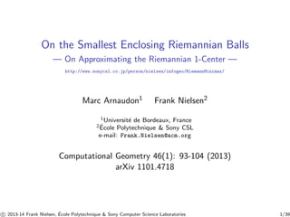
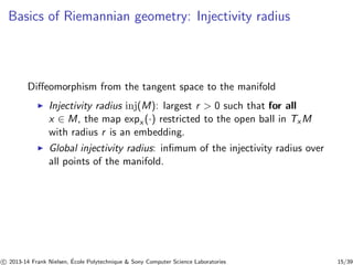
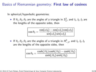
![Basics of Riemannian geometry
◮ (M, g): Riemannian manifold
◮ h·, ·i, Riemannian metric tensor g: definite positive bilinear
form on each tangent space TxM (depends smoothly on x)
◮ k · kx : kuk = hu, ui1/2: Associated norm in TxM
◮ ρ(x, y): metric distance between two points on the manifold
M (length space)
ρ(x, y) = inf Z 1
0 kϕ˙ (t)k dt, ϕ ∈ C1([0, 1],M), ϕ(0) = x, ϕ(1) = y
Parallel transport wrt. Levi-Civita metric connection ∇: ∇g = 0.
c
2013-14 Frank Nielsen, ´E
cole Polytechnique Sony Computer Science Laboratories 10/39](https://image.slidesharecdn.com/smallestenclosingriemannianball-141003080411-phpapp02/85/On-approximating-the-Riemannian-1-center-10-320.jpg)
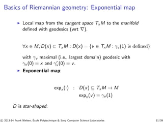
![Basics of Riemannian geometry: Geodesics
◮ Geodesic: smooth path which locally minimizes the distance
between two points. (In general such a curve does not
minimize it globally.)
◮ Given a vector v ∈ TxM with base point x, there is a unique
geodesic started at x with speed v at time 0: t7→ expx (tv) or
t7→ γt(v).
◮ Geodesic on [a, b] is minimal if its length is less or equal to
others. For complete M (i.e., expx (v)), taking x, y ∈ M, there
exists a minimal geodesic from x to y in time 1.
γ·(x, y) : [0, 1] → M, t7→ γt (x, y) with the conditions
γ0(x, y) = x and γ1(x, y) = y.
◮ U ⊆ M is convex if for any x, y ∈ U, there exists a unique
minimal geodesic γ·(x, y) in M from x to y. Geodesic fully
lies in U and depends smoothly on x, y, t.
c
2013-14 Frank Nielsen, ´E
cole Polytechnique Sony Computer Science Laboratories 12/39](https://image.slidesharecdn.com/smallestenclosingriemannianball-141003080411-phpapp02/85/On-approximating-the-Riemannian-1-center-12-320.jpg)
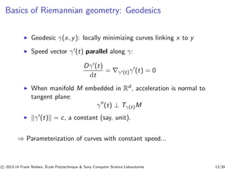
![Basics of Riemannian geometry: Geodesics
Constant speed geodesic γ(t) so that γ(0) = x and γ(ρ(x, y)) = y
(constant speed 1, the unit of length).
x#ty = m = γ(t) : ρ(x,m) = t × ρ(x, y)
For example, in the Euclidean space:
x#ty = (1 − t)x + ty = x + t(y − x) = m
ρE (x,m) = kt(y − x)k = tky − xk = t × ρ(x, y), t ∈ [0, 1]
⇒ m interpreted as a mean (barycenter) between x and y.
c
2013-14 Frank Nielsen, ´E
cole Polytechnique Sony Computer Science Laboratories 14/39](https://image.slidesharecdn.com/smallestenclosingriemannianball-141003080411-phpapp02/85/On-approximating-the-Riemannian-1-center-14-320.jpg)
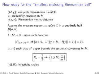
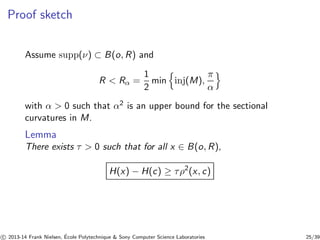
![Riemannian SEB: Existence and uniqueness [1]
Assume
R Rα
Consider farthest point map:
H : M → [0,∞]
x7→ kρ(x, ·)kL∞(ν) (1)
c ∈ B(o, R).
→ c ⊂ CH(supp(ν)) [1] (convex hull)
⇒ center: notion of centrality of the measure
⇒ point set: discrete measure, center → circumcenter
c
2013-14 Frank Nielsen, ´E
cole Polytechnique Sony Computer Science Laboratories 21/39](https://image.slidesharecdn.com/smallestenclosingriemannianball-141003080411-phpapp02/85/On-approximating-the-Riemannian-1-center-21-320.jpg)
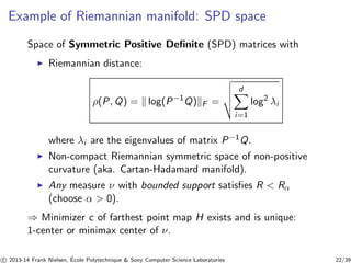
![Generalizing BCA to Riemannian manifolds
a#Mt
b: point γ(t) on the geodesic line segment [ab] wrt M.
Algorithm 4: GeoA
c1 ← choose randomly a point in P;
for i = 2 to l do
nj
// farthest point from ci
si ← argmax=1ρ(ci , pj );
// update the center: walk on the geodesic line
segment [ci , psi ]
ci+1 ← ci#M
1
i+1
psi ;
end
// Return the SEB approximation
return Ball(cl , rl = ρ(cl ,P)) ;
c
2013-14 Frank Nielsen, ´E
cole Polytechnique Sony Computer Science Laboratories 24/39](https://image.slidesharecdn.com/smallestenclosingriemannianball-141003080411-phpapp02/85/On-approximating-the-Riemannian-1-center-24-320.jpg)
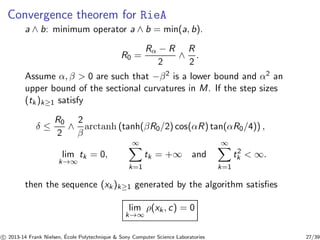
![Stochastic approximation for measures
For x ∈ B(o, R), t7→ γt (v(x, ν)) a unit speed geodesic from
γ0(v(x, ν)) = x to one point y = γH(x)(v(x, ν)) in supp(ν) which
realizes the maximum of the distance from x to supp(ν).
v =
1
H(x)
exp−1
x (y)
RieA:
Fix some δ 0.
◮ Step 1 Choose a starting point x0 ∈ supp(ν) and let
k = 0
◮ Step 2 Choose a step size tk+1 ∈ (0, δ] and let
xk+1 = γtk+1(v(xk , ν)), then do again step 2 with
k ← k + 1.
c
2013-14 Frank Nielsen, ´E
cole Polytechnique Sony Computer Science Laboratories 26/39](https://image.slidesharecdn.com/smallestenclosingriemannianball-141003080411-phpapp02/85/On-approximating-the-Riemannian-1-center-26-320.jpg)
![Case study I: Hyperbolic planar manifold
In Klein disk (projective model), geodesics are straight (euclidean)
lines [11].
ρ(p, q) = arccosh
1 − p⊤q
p(1 − p⊤p)(1 − q⊤q)
where arccosh(x) = log(x + √x2 − 1).
Here, we choose non-constant speed curve parameterization (not
constant-speed geodesic):
˜γt (p, q) = (1 − t)p + tq, t ∈ [0, 1].
⇒ Implement a dichotomy on ˜γt(p, q) to get #t .
c
2013-14 Frank Nielsen, ´E
cole Polytechnique Sony Computer Science Laboratories 28/39](https://image.slidesharecdn.com/smallestenclosingriemannianball-141003080411-phpapp02/85/On-approximating-the-Riemannian-1-center-28-320.jpg)
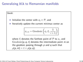
![Case study II: Space of SPD matrices
◮ d × d matrix M Symmetric Positive Definite (SPD) ⇔
M = M⊤ and that for all x6= 0, x⊤Mx 0.
◮ The set of d × d SPD matrices: manifold of dimension
d(d+1)
2 [8]
◮ The geodesic linking (matrix) point P to point Q:
γt(P,Q) = P
1
2 P−1
2 t
2QP−1
P
1
2
where the matrix function h(M) is computed from the
singular value decomposition M = UDV ⊤ (with U and V
unitary matrices and D = diag(λ1, ..., λd ) a diagonal matrix
of eigenvalues) as h(M) = Udiag(h(λ1), ..., h(λd ))V ⊤. For
example, the square root function of a matrix is computed as
M
1
2 = U diag(√λ1, ...,√λd ) V ⊤.
c
2013-14 Frank Nielsen, ´E
cole Polytechnique Sony Computer Science Laboratories 31/39](https://image.slidesharecdn.com/smallestenclosingriemannianball-141003080411-phpapp02/85/On-approximating-the-Riemannian-1-center-31-320.jpg)
![Remark on SPD spaces and hyperbolic geometry
◮ 2D SPD(2) matrix space has dimension d = 3: A positive
cone.
(a, b, c) : a 0, ab − c2 0 ◮ Can be peeled into sheets of dimension 2, each sheet
corresponding to a constant value of the determinant of the
elements [4]
SPD(2) = SSPD(2) × R+,
where SSPD(2) = {a, b, c = √1 − ab) : a 0, ab − c2 = 1}
2 ≥ 1, x1 = a−b
◮ Map to (x0 = a+b
2 , x2 = c) in hyperboloid
model [12], and z = a−b+2ic
2+a+b in Poincar´e disk [12].
c
2013-14 Frank Nielsen, ´E
cole Polytechnique Sony Computer Science Laboratories 34/39](https://image.slidesharecdn.com/smallestenclosingriemannianball-141003080411-phpapp02/85/On-approximating-the-Riemannian-1-center-34-320.jpg)
![Conclusion: Smallest Riemannian Enclosing Ball
◮ Generalize Euclidean 1-center algorithm of [2] to Riemannian
geometry
◮ Proved the convergence under mild assumptions (for
measures/point sets)
◮ Existence of Riemannian core-sets for optimization
◮ 1-center building block for k-center clustering [6]
◮ can be extended to sets of Riemannian (geodesic) balls
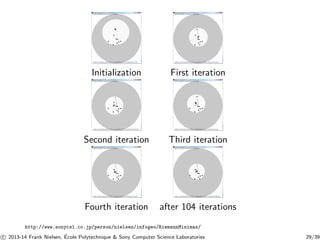
Reproducible research codes with interactive demos:
http://www.sonycsl.co.jp/person/nielsen/infogeo/RiemannMinimax/
c
2013-14 Frank Nielsen, ´E
cole Polytechnique Sony Computer Science Laboratories 35/39](https://image.slidesharecdn.com/smallestenclosingriemannianball-141003080411-phpapp02/85/On-approximating-the-Riemannian-1-center-35-320.jpg)

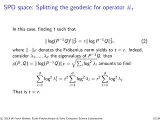
This document discusses algorithms for finding the smallest enclosing ball that fully covers a set of points on a Riemannian manifold. It begins by reviewing Euclidean smallest enclosing ball algorithms, then extends the concept to Riemannian manifolds. Coreset approximations are discussed as well as gradient descent algorithms. The document provides background on Riemannian geometry concepts needed like geodesics, exponential maps, and curvature. Overall, it presents algorithms to generalize the smallest enclosing ball problem to points on Riemannian manifolds.