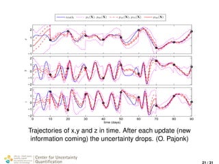
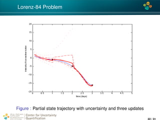
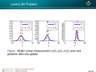
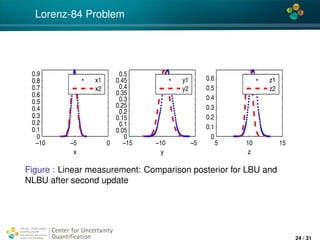
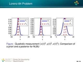
The document discusses non-linear approximation methods for Bayesian updates, emphasizing the need for computational efficiency in Bayesian inference as conventional methods like MCMC can be costly. It proposes using polynomial chaos coefficients and focuses on improving parameter identification with conditional expectations in a Bayesian framework. Multiple examples illustrate the application of these concepts to uncertain systems, including the Lorenz system and elliptic PDE scenarios.

1. NON-LINEAR APPROXIMATION OF
BAYESIAN UPDATE
Alexander Litvinenko1, Hermann G. Matthies2, Elmar Zander2
Center for Uncertainty
Quantification
ntification Logo Lock-up
http://sri-uq.kaust.edu.sa/
1Extreme Computing Research Center, KAUST,
2Institute of Scientific Computing, TU Braunschweig, Brunswick, Germany

2. 4*
KAUST
Figure : KAUST campus, 7 years old, approx. 7000 people (include
1700 kids), 100 nations, 36 km2
.
Center for Uncertainty
Quantification
ation Logo Lock-up
2 / 31

3. 4*
Stochastic Numerics Group at KAUST
Center for Uncertainty
Quantification
ation Logo Lock-up
3 / 31

4. Center for Uncertainty
Quantification
ation Logo Lock-up
4 / 31

5. 4*
A BIG picture
1. Computing the full Bayesian update is very expensive
(MCMC is expensive)
2. Look for a cheap surrogate (linear, quadratic, cubic,...
approx.)
3. Kalman filter is a particular case
4. Do Bayesian update of Polynomial Chaos Coefficients!
(not probability densities!)
5. Consider non-Gaussian cases
Center for Uncertainty
Quantification
ation Logo Lock-up
5 / 31

6. 4*
History
1. O. Pajonk, B. V. Rosic, A. Litvinenko, and H. G. Matthies, A
Deterministic Filter for Non-Gaussian Bayesian Estimation,
Physica D: Nonlinear Phenomena, Vol. 241(7), pp. 775-788,
2012.
2. B. V. Rosic, A. Litvinenko, O. Pajonk and H. G. Matthies,
Sampling Free Linear Bayesian Update of Polynomial Chaos
Representations, J. of Comput. Physics, Vol. 231(17), 2012 , pp
5761-5787
3. A. Litvinenko and H. G. Matthies, Inverse problems and
uncertainty quantification
http://arxiv.org/abs/1312.5048, 2013
4. H. G. Matthies, E. Zander, B.V. Rosic, A. Litvinenko, Parameter
estimation via conditional expectation - A Bayesian Inversion,
accepted to AMOS-D-16-00015, 2016.
5. H. G. Matthies, E. Zander, B.V. Rosic, A. Litvinenko, Bayesian
parameter estimation via filtering and functional approximation,
Tehnicki vjesnik 23, 1(2016), 1-17.Center for Uncertainty
Quantification
ation Logo Lock-up
6 / 31

7. 4*
Setting for the identification process
General idea:
We observe / measure a system, whose structure we know in
principle.
The system behaviour depends on some quantities
(parameters),
which we do not know ⇒ uncertainty.
We model (uncertainty in) our knowledge in a Bayesian setting:
as a probability distribution on the parameters.
We start with what we know a priori, then perform a
measurement.
This gives new information, to update our knowledge
(identification).
Update in probabilistic setting works with conditional
probabilities
⇒ Bayes’s theorem.
Repeated measurements lead to better identification.
Center for Uncertainty
Quantification
ation Logo Lock-up
7 / 31

8. 4*
Mathematical setup
Consider
A(u; q) = f ⇒ u = S(f; q),
where S is solution operator.
Operator depends on parameters q ∈ Q,
hence state u ∈ U is also function of q:
Measurement operator Y with values in Y:
y = Y(q; u) = Y(q, S(f; q)).
Examples of measurements:
y(ω) = D0
u(ω, x)dx, or u in few points
Center for Uncertainty
Quantification
ation Logo Lock-up
8 / 31

9. 4*
Inverse problem
For given f, measurement y is just a function of q.
This function is usually not invertible ⇒ ill-posed problem,
measurement y does not contain enough information.
In Bayesian framework state of knowledge modelled in a
probabilistic way,
parameters q are uncertain, and assumed as random.
Bayesian setting allows updating / sharpening of information
about q when measurement is performed.
The problem of updating distribution—state of knowledge of q
becomes well-posed.
Can be applied successively, each new measurement y and
forcing f —may also be uncertain—will provide new
information.
Center for Uncertainty
Quantification
ation Logo Lock-up
9 / 31

10. 4*
Conditional probability and expectation
With state u a RV, the quantity to be measured
y(ω) = Y(q(ω), u(ω)))
is also uncertain, a random variable.
Noisy data: ˆy + (ω), where ˆy is the “true” value and a random
error .
Forecast of the measurement: z(ω) = y(ω) + (ω).
Classically, Bayes’s theorem gives conditional probability
P(Iq|Mz) =
P(Mz|Iq)
P(Mz)
P(Iq) (or πq(q|z) =
p(z|q)
Zs
pq(q))
expectation with this posterior measure is conditional
expectation. Kolmogorov starts from conditional expectation
E (·|Mz),
from this conditional probability via P(Iq|Mz) = E χIq
|Mz .
Center for Uncertainty
Quantification
ation Logo Lock-up
10 / 31

11. 4*
Conditional expectation
The conditional expectation is defined as
orthogonal projection onto the closed subspace L2(Ω, P, σ(z)):
E(q|σ(z)) := PQ∞ q = argmin˜q∈L2(Ω,P,σ(z)) q − ˜q 2
L2
The subspace Q∞ := L2(Ω, P, σ(z)) represents the available
information.
The update, also called the assimilated value
qa(ω) := PQ∞ q = E(q|σ(z)),
and represents new state of knowledge after the measurement.
Doob-Dynkin: Q∞ = {ϕ ∈ Q : ϕ = φ ◦ z, φ measurable}.
Center for Uncertainty
Quantification
ation Logo Lock-up
11 / 31

12. 4*
Polynomial Chaos Expansion (Norbert Wiener, 1938)
Multivariate Hermite polynomials were used to approximate
random fields/stochastic processes with Gaussian random
variables. According to Cameron and Martin theorem PCE
expansion converges in the L2 sense.
Let Y(x, θ), θ = (θ1, ..., θM, ...), is approximated:
Y(x, θ) =
β∈Jm,p
Hβ(θ)Yβ(x), |Jm,p| =
(m + p)!
m!p!
,
Hβ(θ) = M
k=1 hβk
(θk ),
Yβ(x) =
1
β! Θ
Hβ(θ)Y(x, θ) P(dθ).
Yβ(x) ≈
1
β!
Nq
i=1
Hβ(θi)Y(x, θi)wi.
Center for Uncertainty
Quantification
ation Logo Lock-up
12 / 31

13. 4*
Numerical computation of NLBU
Look for ϕ such that q(ξ) = ϕ(z(ξ)), z(ξ) = y(ξ) + ε(ω):
ϕ ≈ ˜ϕ =
α∈Jp
ϕαΦα(z(ξ)) (1)
and minimize q(ξ) − ˜ϕ(z(ξ)) 2, where Φα are polynomials
(e.g. Hermite, Laguerre, Chebyshev or something else). Taking
derivatives with respect to ϕα:
∂
∂ϕα
q(ξ) − ˜ϕ(z(ξ)), q(ξ) − ˜ϕ(z(ξ)) = 0 ∀α ∈ Jp (2)
Inserting representation for ˜ϕ, obtain
Center for Uncertainty
Quantification
ation Logo Lock-up
13 / 31

14. 4*
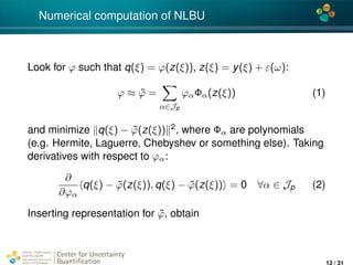
Numerical computation of NLBU
∂
∂ϕα
E

q2
(ξ) − 2
β∈J
qϕβΦβ(z) +
β,γ∈J
ϕβϕγΦβ(z)Φγ(z)


= 2E

−qΦα(z) +
β∈J
ϕβΦβ(z)Φα(z)


= 2


β∈J
E [Φβ(z)Φα(z)] ϕβ − E [qΦα(z)]

 = 0 ∀α ∈ J
E [Φβ(z)Φα(z)] ϕβ = E [qΦα(z)]
Center for Uncertainty
Quantification
ation Logo Lock-up
14 / 31

15. 4*
Numerical computation of NLBU
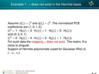
Now, rewriting the last sum in a matrix form, obtain the linear
system of equations (=: A) to compute coefficients ϕβ:



... ... ...
... E [Φα(z(ξ))Φβ(z(ξ))]
...
... ... ...







...
ϕβ
...



 =




...
E [q(ξ)Φα(z(ξ))]
...



 ,
where α, β ∈ J , A is of size |J | × |J |.
Center for Uncertainty
Quantification
ation Logo Lock-up
15 / 31

16. 4*
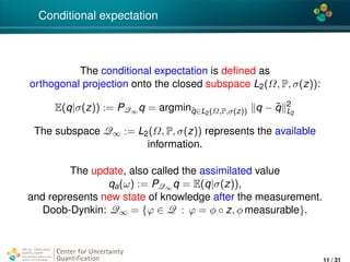
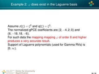
Numerical computation of NLBU
Using the same quadrature rule of order q for each element of
A, we can write
A = E ΦJα (z(ξ))ΦJβ
(z(ξ))T
≈
NA
i=1
wA
i ΦJα (zi)ΦJβ
(zi)T
, (3)
where (wA
i , ξi) are weights and quadrature points, zi := z(ξi)
and ΦJα (zi) := (...Φα(z(ξi))....)T is a vector of length |Jα|.
b = E [q(ξ)ΦJα (z(ξ))] ≈
Nb
i=1
wb
i q(ξi)ΦJα (zi), (4)
where ΦJα (z(ξi)) := (..., Φα(z(ξi)), ...), α ∈ Jα.
Center for Uncertainty
Quantification
ation Logo Lock-up
16 / 31

17. 4*
Numerical computation of NLBU
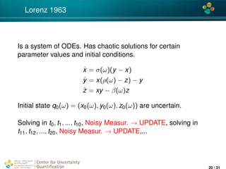
We can write the Eq. 15 with the right-hand side in Eq. 4 in the
compact form:
[ΦA] [diag(...wA
i ...)] [ΦA]T




...
ϕβ
...



 = [Φb]


wb
0 q(ξ0)
...
wb
Nb q(ξNb )

 (5)
[ΦA] ∈ RJα×NA
, [diag(...wA
i ...)] ∈ RNA×NA
, [Φb] ∈ RJα×Nb
,
[wb
0 q(ξ0)...wb
Nb q(ξNb )] ∈ RNb
.
Solving Eq. 5, obtain vector of coefficients (...ϕβ...)T for all β.
Finally, the assimilated parameter qa will be
qa = qf + ˜ϕ(ˆy) − ˜ϕ(z), (6)
z(ξ) = y(ξ) + ε(ω), ˜ϕ = β∈Jp
ϕβΦβ(z(ξ))
Center for Uncertainty
Quantification
ation Logo Lock-up
17 / 31

18. 4*
Example 1: ϕ does not exist in the Hermite basis
Assume z(ξ) = ξ2 and q(ξ) = ξ3. The normalized PCE
coefficients are (1, 0, 1, 0)
(ξ2 = 1 · H0(ξ) + 0 · H1(ξ) + 1 · H2(ξ) + 0 · H3(ξ))
and (0, 3, 0, 1)
(ξ3 = 0 · H0(ξ) + 3 · H1(ξ) + 0 · H2(ξ) + 1 · H3(ξ)).
For such data the mapping ϕ does not exist. The matrix A is
close to singular.
Support of Hermite polynomials (used for Gaussian RVs) is
(−∞, ∞).
Center for Uncertainty
Quantification
ation Logo Lock-up
18 / 31

19. 4*
Example 2: ϕ does exist in the Laguerre basis
Assume z(ξ) = ξ2 and q(ξ) = ξ3.
The normalized gPCE coefficients are (2, −4, 2, 0) and
(6, −18, 18, −6).
For such data the mapping mapping ϕ of order 8 and higher
produces a very accurate result.
Support of Laguerre polynomials (used for Gamma RVs) is
[0, ∞).
Center for Uncertainty
Quantification
ation Logo Lock-up
19 / 31

20. 4*
Lorenz 1963
Is a system of ODEs. Has chaotic solutions for certain
parameter values and initial conditions.
˙x = σ(ω)(y − x)
˙y = x(ρ(ω) − z) − y
˙z = xy − β(ω)z
Initial state q0(ω) = (x0(ω), y0(ω), z0(ω)) are uncertain.
Solving in t0, t1, ..., t10, Noisy Measur. → UPDATE, solving in
t11, t12, ..., t20, Noisy Measur. → UPDATE,...
Center for Uncertainty
Quantification
ation Logo Lock-up
20 / 31

21. Trajectories of x,y and z in time. After each update (new
information coming) the uncertainty drops. (O. Pajonk)
Center for Uncertainty
Quantification
ation Logo Lock-up
21 / 31

22. 4*
Lorenz-84 Problem
Figure : Partial state trajectory with uncertainty and three updates
Center for Uncertainty
Quantification
ation Logo Lock-up
22 / 31

23. 4*
Lorenz-84 Problem
10 0 10
0
0.1
0.2
0.3
0.4
0.5
0.6
0.7
0.8
x
20 0 20
0
0.05
0.1
0.15
0.2
0.25
0.3
0.35
0.4
0.45
y
0 10 20
0
0.1
0.2
0.3
0.4
0.5
0.6
0.7
0.8
0.9
1
z
xf
x
a
yf
y
a
zf
z
a
Figure : NLBU: Linear measurement (x(t), y(t), z(t)): prior and
posterior after one update
Center for Uncertainty
Quantification
ation Logo Lock-up
23 / 31

24. 4*
Lorenz-84 Problem
10 5 0
0
0.1
0.2
0.3
0.4
0.5
0.6
0.7
0.8
0.9
x
x1
x2
15 10 5
0
0.05
0.1
0.15
0.2
0.25
0.3
0.35
0.4
0.45
0.5
y
y1
y2
5 10 15
0
0.1
0.2
0.3
0.4
0.5
0.6
z
z1
z2
Figure : Linear measurement: Comparison posterior for LBU and
NLBU after second update
Center for Uncertainty
Quantification
ation Logo Lock-up
24 / 31

25. 4*
Lorenz-84 Problem
20 0 20
0
0.02
0.04
0.06
0.08
0.1
0.12
0.14
0.16
x
50 0 50
0
0.01
0.02
0.03
0.04
0.05
0.06
0.07
0.08
0.09
y
0 10 20
0
0.02
0.04
0.06
0.08
0.1
0.12
0.14
0.16
0.18
z
xf
x
a
yf
y
a
zf
z
a
Figure : Quadratic measurement (x(t)2
, y(t)2
, z(t)2
): Comparison of
a priori and a posterior for NLBU
Center for Uncertainty
Quantification
ation Logo Lock-up
25 / 31

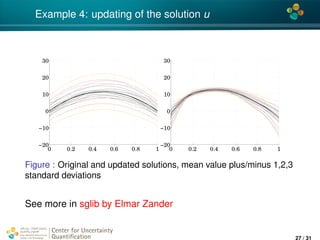
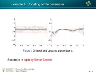
26. 4*
Example 4: 1D elliptic PDE with uncertain coeffs
Taken from Stochastic Galerkin Library (sglib), by Elmar Zander
(TU Braunschweig)
− · (κ(x, ξ) u(x, ξ)) = f(x, ξ), x ∈ [0, 1]
Measurements are taken at x1 = 0.2, and x2 = 0.8. The means
are y(x1) = 10, y(x2) = 5 and the variances are 0.5 and 1.5
correspondingly.
Center for Uncertainty
Quantification
ation Logo Lock-up
26 / 31

27. 4*
Example 4: updating of the solution u
0 0.2 0.4 0.6 0.8 1
−20
−10
0
10
20
30
0 0.2 0.4 0.6 0.8 1
−20
−10
0
10
20
30
Figure : Original and updated solutions, mean value plus/minus 1,2,3
standard deviations
See more in sglib by Elmar Zander
Center for Uncertainty
Quantification
ation Logo Lock-up
27 / 31

28. 4*
Example 4: Updating of the parameter
0 0.2 0.4 0.6 0.8 1
−1
−0.5
0
0.5
1
1.5
2
0 0.2 0.4 0.6 0.8 1
−1
−0.5
0
0.5
1
1.5
2
Figure : Original and updated parameter q.
See more in sglib by Elmar Zander
Center for Uncertainty
Quantification
ation Logo Lock-up
28 / 31

29. 4*
Conclusion about NLBU
+ Step 1. Introduced a way to derive MMSE ϕ (as a linear,
quadratic, cubic etc approximation, i. e. compute
conditional expectation of q, given measurement Y.
Step 2. Apply ϕ to identify parameter q
+ All ingredients can be given as gPC.
+ we apply it to solve inverse problems (ODEs and PDEs).
- Stochastic dimension grows up very fast.
Center for Uncertainty
Quantification
ation Logo Lock-up
29 / 31

30. 4*
Acknowledgment
I used a Matlab toolbox for stochastic Galerkin methods (sglib)
https://github.com/ezander/sglib
Alexander Litvinenko and his research work was supported by
the King Abdullah University of Science and Technology
(KAUST), SRI-UQ and ECRC centers.
Center for Uncertainty
Quantification
ation Logo Lock-up
30 / 31

31. 4*
Literature
1. Bojana Rosic, Jan Sykora, Oliver Pajonk, Anna Kucerova
and Hermann G. Matthies, Comparison of Numerical
Approaches to Bayesian Updating, report on
www.wire.tu-bs.de, 2014
2. A. Litvinenko and H. G. Matthies, Inverse problems and
uncertainty quantification
http://arxiv.org/abs/1312.5048, 2013
3. L. Giraldi, A. Litvinenko, D. Liu, H. G. Matthies, A. Nouy, To
be or not to be intrusive? The solution of parametric and
stochastic equations - the ”plain vanilla” Galerkin case,
http://arxiv.org/abs/1309.1617, 2013
4. O. Pajonk, B. V. Rosic, A. Litvinenko, and H. G. Matthies, A
Deterministic Filter for Non-Gaussian Bayesian Estimation,
Physica D: Nonlinear Phenomena, Vol. 241(7), pp.
775-788, 2012.
5. B. V. Rosic, A. Litvinenko, O. Pajonk and H. G. Matthies,
Sampling Free Linear Bayesian Update of PolynomialCenter for Uncertainty
Quantification
ation Logo Lock-up
31 / 31

32. 4*
Literature
1. PCE of random coefficients and the solution of stochastic partial
differential equations in the Tensor Train format, S. Dolgov, B. N.
Khoromskij, A. Litvinenko, H. G. Matthies, 2015/3/11,
arXiv:1503.03210
2. Efficient analysis of high dimensional data in tensor formats, M.
Espig, W. Hackbusch, A. Litvinenko, H.G. Matthies, E. Zander Sparse
Grids and Applications, 31-56, 40, 2013
3. Application of hierarchical matrices for computing the
Karhunen-Loeve expansion, B.N. Khoromskij, A. Litvinenko, H.G.
Matthies, Computing 84 (1-2), 49-67, 31, 2009
4. Efficient low-rank approximation of the stochastic Galerkin matrix
in tensor formats, M. Espig, W. Hackbusch, A. Litvinenko, H.G.
Matthies, P. Waehnert, Comp. & Math. with Appl. 67 (4), 818-829,
2012
5. Numerical Methods for Uncertainty Quantification and Bayesian
Update in Aerodynamics, A. Litvinenko, H. G. Matthies, Book
”Management and Minimisation of Uncertainties and Errors in
Numerical Aerodynamics” pp 265-282, 2013
Center for Uncertainty
Quantification
ation Logo Lock-up
32 / 31