STATISTICS OF CLIMATE EXTREMES:
MULTIVARIATE AND SPATIAL EXTREMES
Richard L Smith
Departments of STOR and Biostatistics, University
of North Carolina at Chapel Hill
and
Statistical and Applied Mathematical Sciences
Institute (SAMSI)
SAMSI Graduate Class
November 28, 2017
1
Heffernan and Tawn (2004)
1
MULTIVARIATE EXTREMES
AND MAX-STABLE PROCESSES
I Limit theory for multivariate sample maxima
II Alternative formulations of multivariate extreme value theory
III Max-stable processes
2
Multivariate extreme value theory applies when we are interested
in the joint distribution of extremes from several random vari-
ables.
Examples:
• Winds and waves on an offshore structure
• Meteorological variables, e.g. temperature and precipitation
• Air pollution variables, e.g. ozone and sulfur dioxide
• Finance, e.g. price changes in several stocks or indices
• Spatial extremes, e.g. joint distributions of extreme precipi-
tation at several locations
3
I LIMIT THEOREMS FOR MULTIVARIATE SAMPLE
MAXIMA
Let Yi = (Yi1...YiD)T be i.i.d. D-dimensional vectors, i = 1, 2, ...
Mnd = max{Y1d, ..., Ynd}(1 ≤ d ≤ D) — d’th-component maxi-
mum
Look for constants and, bnd such that
Pr
Mnd − bnd
and
≤ xd, d = 1, ..., D → G(x1, ..., xD).
Vector notation:
Pr
Mn − bn
an
≤ x → G(x).
4
Two general points:
1. If G is a multivariate extreme value distribution, then each
of its marginal distributions must be one of the univariate
extreme value distributions, and therefore can be represented
in GEV form
2. The form of the limiting distribution is invariant under mono-
tonic transformation of each component. Therefore, without
loss of generality we can transform each marginal distribu-
tion into a specified form. For most of our applications, it is
convenient to assume the Fr´echet form:
Pr{Xd ≤ x} = exp(−x−α), x > 0, d = 1, ..., D.
Here α > 0. The case α = 1 is called unit Fr´echet.
5
Representations of Limit Distributions
Any MEVD with unit Fr´echet margins may be written as
G(x) = exp {−V (x)} , (1)
V (x) =
SD
max
d=1,...,D
wj
xj
dH(w), (2)
where SD = {(x1, ..., xD) : x1 ≥ 0, ..., xD ≥ 0, x1 + ... + xD = 1}
and H is a measure on SD.
The function V (x) is called the exponent measure and formula
(2) is the Pickands representation. If we fix d ∈ {1, ..., D} with
0 < xd < ∞, and define xd = +∞ for d = d , then
V (x) =
SD
max
d=1,...,D
wd
xd
dH(w) =
1
xd SD
wd dH(w)
so to ensure correct marginal distributions we must have
SD
wddH(w) = 1, d = 1, ..., D. (3)
6
Note that
kV (x) = V
x
k
(which is in fact another characterization of V ) so
Gk(x) = exp(−kV (x))
= exp −V
x
k
= G
x
k
.
Hence G is max-stable. In particular, if X1, ..., Xk are i.i.d. from
G, then max{X1, ..., Xk} (vector of componentwise maxima) has
the same distribution as kX1.
7
The Pickands Dependence Function
In the two-dimensional case (with unit Fr´echet margins) there is
an alternative representation due to Pickands:
Pr{X1 ≤ x1, X2 ≤ x2} = exp −
1
x1
+
1
x2
A
x1
x1 + x2
where A is a convex function on [0,1] such that A(0) = A(1) =
1, 1
2 ≤ A 1
2 ≤ 1.
The value of A 1
2 is often taken as a measure of the strength of
dependence: A 1
2 = 1
2 is “perfect dependence” while A 1
2 = 1
is independence.
8
I.a EXAMPLES
9
Logistic (Gumbel and Goldstein, 1964)
V (x) =


D
d=1
x−r
d


1/r
, r ≥ 1.
Check:
1. V (x/k) = kV (x)
2. V ((+∞, +∞, ..., xd, ..., +∞, +∞) = x−1
d
3. e−V (x) is a valid c.d.f.
Limiting cases:
• r = 1: independent components
• r → ∞: the limiting case when Xi1 = Xi2 = ... = XiD with
probability 1.
10
Asymmetric logistic (Tawn 1990)
V (x) =
c∈C



i∈c
θi,c
xi
rc



1/rc
,
where C is the class of non-empty subsets of {1, ..., D}, rc ≥
1, θi,c = 0 if i /∈ c, θi,c ≥ 0, c∈C θi,c = 1 for each i.
Negative logistic (Joe 1990)
V (x) =
1
xj
+
c∈C: |c|≥2
(−1)|c|



i∈c
θi,c
xi
rc



1/rc
,
rc ≤ 0, θi,c = 0 if i /∈ c, θi,c ≥ 0, c∈C(−1)|c|θi,c ≤ 1 for each i.
11
Tilted Dirichlet (Coles and Tawn 1991)
A general construction: Suppose h∗ is an arbitrary positive func-
tion on Sd with md = SD
udh∗(u)du < ∞, then define
h(w) = ( mkwk)−(D+1)
D
d=1
mdh∗ m1w1
mkwk
, ...,
mDwD
mkwk
.
h is density of positive measure H, SD
uddH(u) = 1 each d.
As a special case of this, they considered Dirichlet density
h∗(u) =
Γ( αj)
d Γ(αd)
D
d=1
u
αd−1
d .
Leads to
h(w) =
D
d=1
αd
Γ(αd)
·
Γ( αd + 1)
( αdwd)D+1
D
d=1
αdwd
αkwk
αd−1
.
Disadvantage: need for numerical integration
12
I.b ESTIMATION
• Parametric
• Non/semi-parametric
Both approaches have problems, e.g. nonregular behavior of
MLE even in finite-parameter problems; curse of dimensionality
if D large.
Typically proceed by transforming margins to unit Fr´echet first,
though there are advantages in joint estimation of marginal dis-
tributions and dependence structure (Shi 1995)
13
II ALTERNATIVE FORMULATIONS OF
MULTIVARIATE EXTREMES
14
• Ledford-Tawn-Ramos approach
• Heffernan-Tawn approach
15
The first paper to suggest that multivariate extreme value theory
(as defined so far) might not be general enough was Ledford and
Tawn (1996).
Suppose (Z1, Z2) are a bivariate random vector with unit Fr´echet
margins. Traditional cases lead to
Pr{Z1 > r, Z2 > r} ∼
const. × r−1 dependent cases
const. × r−2 exact independent
The first case covers all bivariate extreme value distributions ex-
cept the independent case. However, Ledford and Tawn showed
by example that for a number of cases of practical interest,
Pr{Z1 > r, Z2 > r} ∼ L(r)r−1/η,
where L is a slowly varying function (L(rx)
L(r)
→ 1 as r → ∞) and
η ∈ (0, 1].
Estimation: used fact that 1/η is Pareto index for min(Z1, Z2).
16
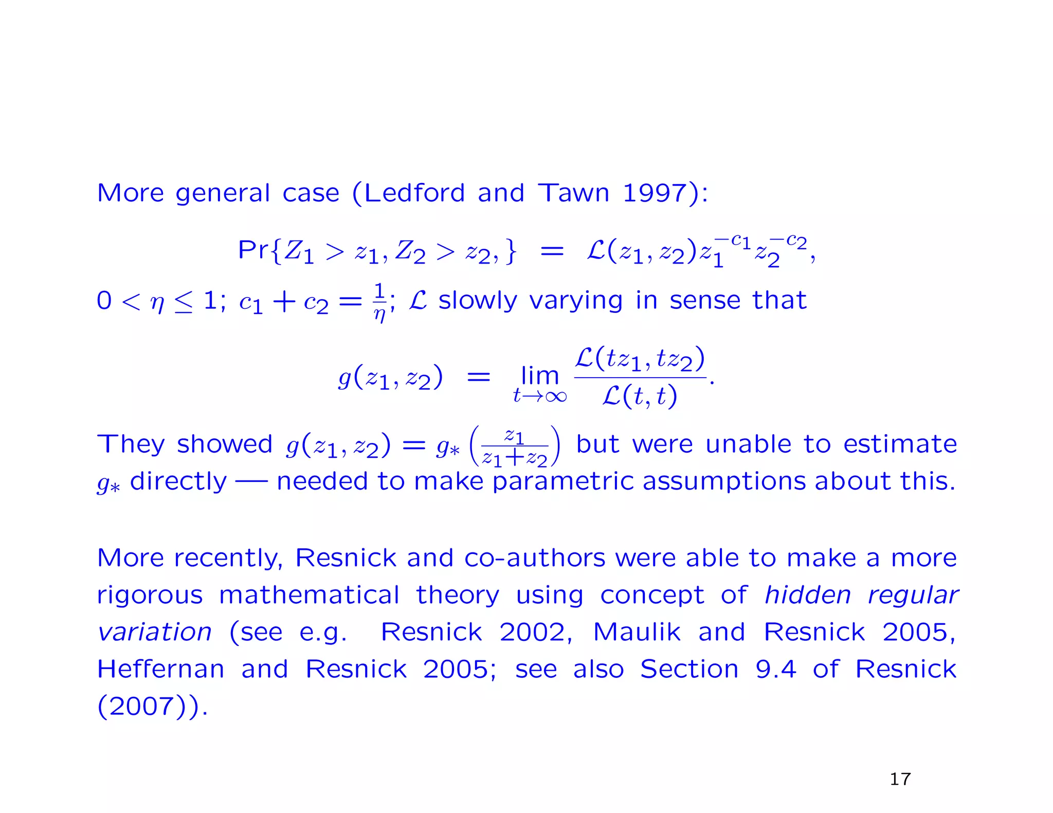
More general case (Ledford and Tawn 1997):
Pr{Z1 > z1, Z2 > z2, } = L(z1, z2)z
−c1
1 z
−c2
2 ,
0 < η ≤ 1; c1 + c2 = 1
η; L slowly varying in sense that
g(z1, z2) = lim
t→∞
L(tz1, tz2)
L(t, t)
.
They showed g(z1, z2) = g∗
z1
z1+z2
but were unable to estimate
g∗ directly — needed to make parametric assumptions about this.
More recently, Resnick and co-authors were able to make a more
rigorous mathematical theory using concept of hidden regular
variation (see e.g. Resnick 2002, Maulik and Resnick 2005,
Heffernan and Resnick 2005; see also Section 9.4 of Resnick
(2007)).
17
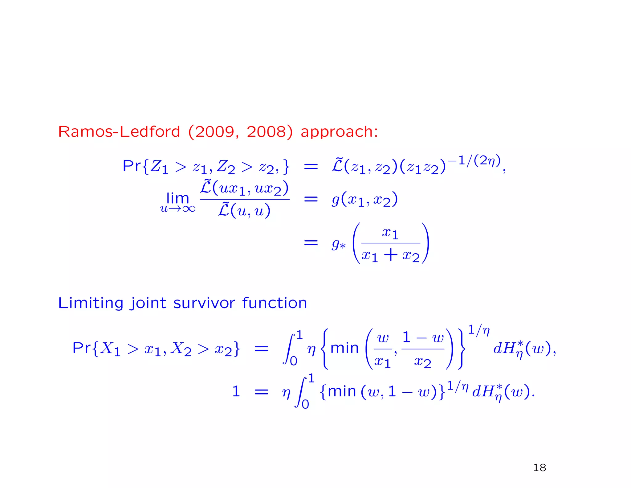
Ramos-Ledford (2009, 2008) approach:
Pr{Z1 > z1, Z2 > z2, } = ˜L(z1, z2)(z1z2)−1/(2η),
lim
u→∞
˜L(ux1, ux2)
˜L(u, u)
= g(x1, x2)
= g∗
x1
x1 + x2
Limiting joint survivor function
Pr{X1 > x1, X2 > x2} =
1
0
η min
w
x1
,
1 − w
x2
1/η
dH∗
η(w),
1 = η
1
0
{min (w, 1 − w)}1/η
dH∗
η(w).
18
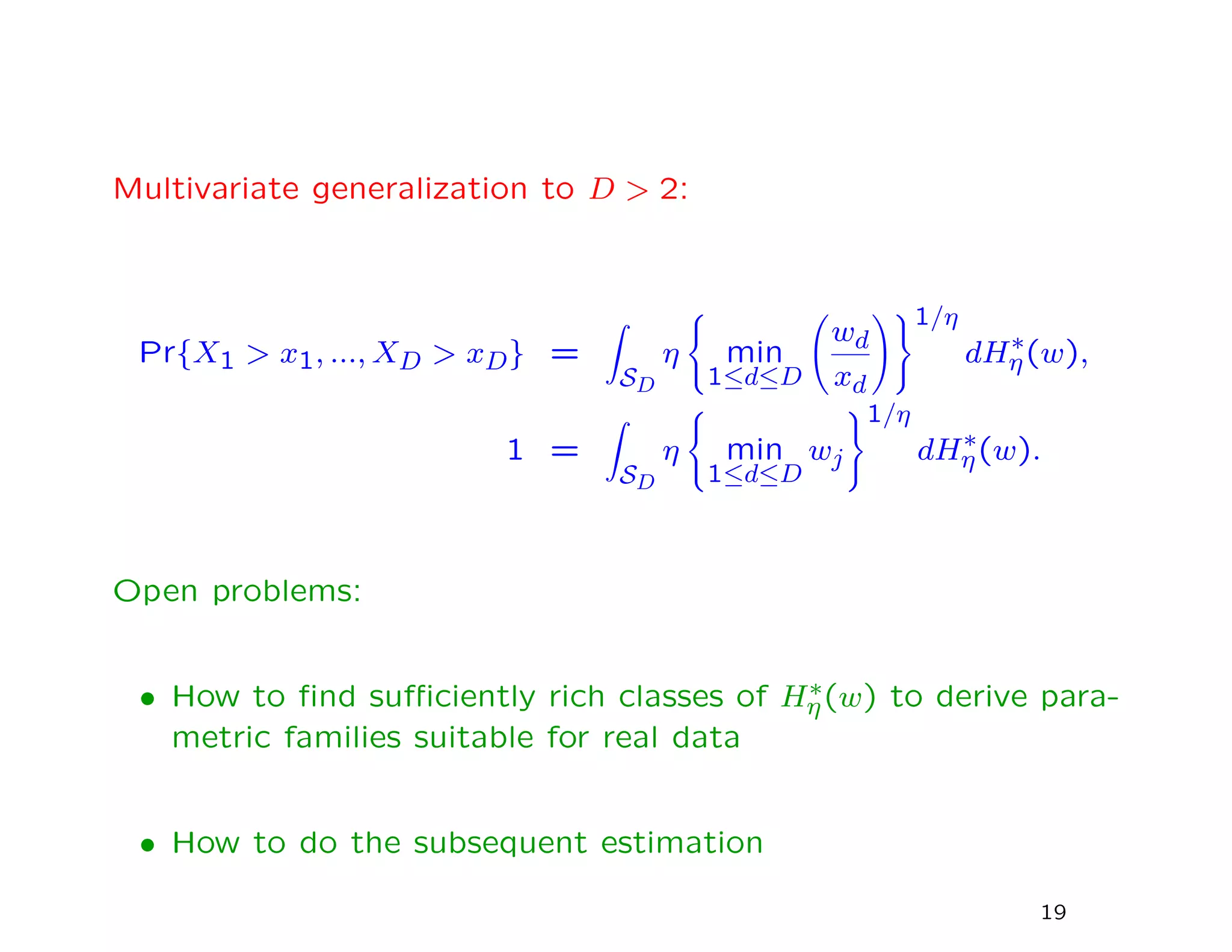
Multivariate generalization to D > 2:
Pr{X1 > x1, ..., XD > xD} =
SD
η min
1≤d≤D
wd
xd
1/η
dH∗
η(w),
1 =
SD
η min
1≤d≤D
wj
1/η
dH∗
η(w).
Open problems:
• How to find sufficiently rich classes of H∗
η(w) to derive para-
metric families suitable for real data
• How to do the subsequent estimation
19
The Heffernan-Tawn approach
Reference:
A conditional approach for multivariate extreme values, by Janet
Heffernan and Jonathan Tawn, J.R. Statist. Soc. B 66, 497–
546 (with discussion)
20
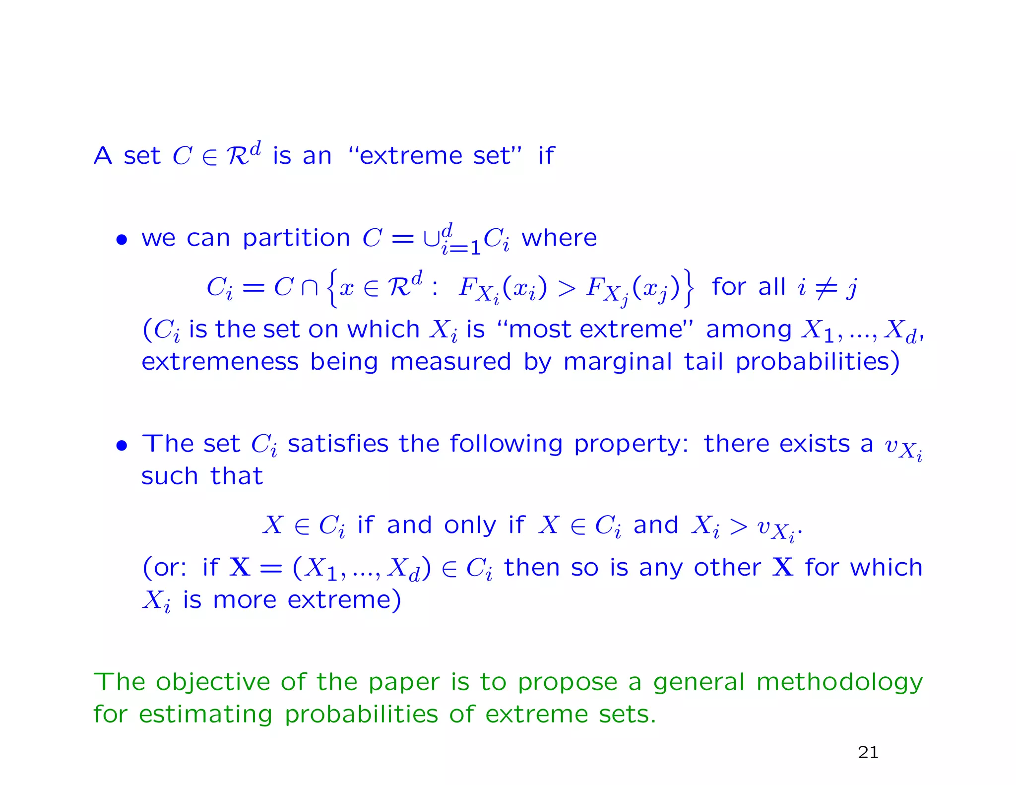
A set C ∈ Rd is an “extreme set” if
• we can partition C = ∪d
i=1Ci where
Ci = C ∩ x ∈ Rd : FXi
(xi) > FXj
(xj) for all i = j
(Ci is the set on which Xi is “most extreme” among X1, ..., Xd,
extremeness being measured by marginal tail probabilities)
• The set Ci satisfies the following property: there exists a vXi
such that
X ∈ Ci if and only if X ∈ Ci and Xi > vXi
.
(or: if X = (X1, ..., Xd) ∈ Ci then so is any other X for which
Xi is more extreme)
The objective of the paper is to propose a general methodology
for estimating probabilities of extreme sets.
21
Marginal distributions
• Standard “GPD” model fit: define a threshold uXi
and as-
sume
Pr{Xi > uXi
+ x | Xi > uXi
} = 1 + ξi
x
βi
−1/ξi
+
for x > 0.
• Also estimate FXi
(x) by empirical CDF for x < uXi
.
• Combine together for an estimate ˆFXi
(x) across the entire
range of x.
• Apply componentwise probability integral transform — Yi =
− log[− log{ ˆFXi
(Xi)}] to have approximately Gumbel margins
(i.e. Pr{Yi ≤ yi} ≈ exp(−e−y)).
• Henceforth assume marginal distributions are exactly Gumbel
and concentrate on dependence among Y1, ..., Yd.
22
Existing techniques
Most existing extreme value methods with Gumbel margins re-
duce to
Pr{Y ∈ t + A} ≈ e−t/ηY Pr{Y ∈ A}
for some ηY ∈ (0, 1]. Ledford-Tawn classification:
• ηY = 1 is asymptotic dependence (includes all conventional
multivariate extreme value distributions)
• 1
d < ηY < 1 — positive extremal dependence
• 0 < ηY < 1
d — negative extremal dependence
• ηY = 1
d — near extremal independence
Disadvantage: doesn’t work for extreme sets that are not simul-
taneously extreme in all components
23
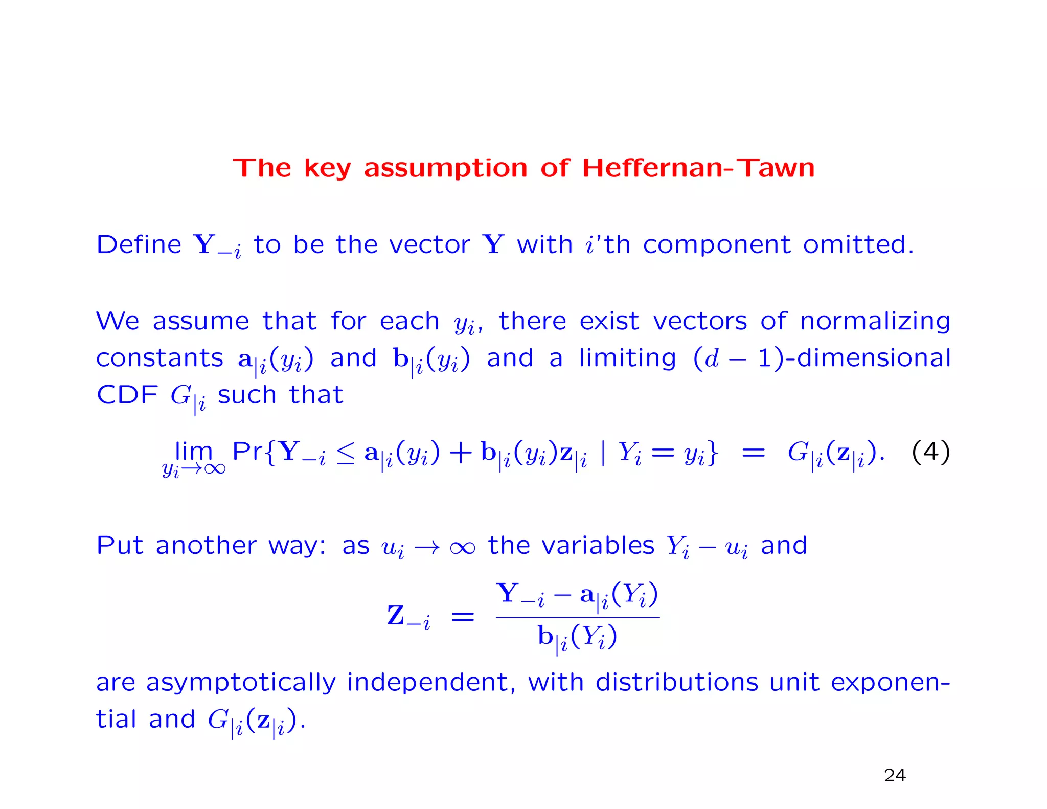
The key assumption of Heffernan-Tawn
Define Y−i to be the vector Y with i’th component omitted.
We assume that for each yi, there exist vectors of normalizing
constants a|i(yi) and b|i(yi) and a limiting (d − 1)-dimensional
CDF G|i such that
lim
yi→∞
Pr{Y−i ≤ a|i(yi) + b|i(yi)z|i | Yi = yi} = G|i(z|i). (4)
Put another way: as ui → ∞ the variables Yi − ui and
Z−i =
Y−i − a|i(Yi)
b|i(Yi)
are asymptotically independent, with distributions unit exponen-
tial and G|i(z|i).
24
Examples in case d = 2
Distribution η a(y) b(y)
Perfect pos. dependence 1 y 1
Bivariate EVD 1 y 1
Bivariate normal, ρ > 0 1+ρ
2 ρ2y y1/2
Inverted logistic, α ∈ (0, 1] 2−α 0 y1−α
Independent 1
2 0 1
Morganstern 1
2 0 1
Bivariate normal, ρ < 0 1+ρ
2 − log(ρ2y) y−1/2
Perfect neg. dependence 0 − log(y) 1
Key observation: in all cases b(y) = yb for some b and a(y) is
either 0 or a linear function of y or − log y (for more precise
conditions see equation (3.8) of the paper)
25
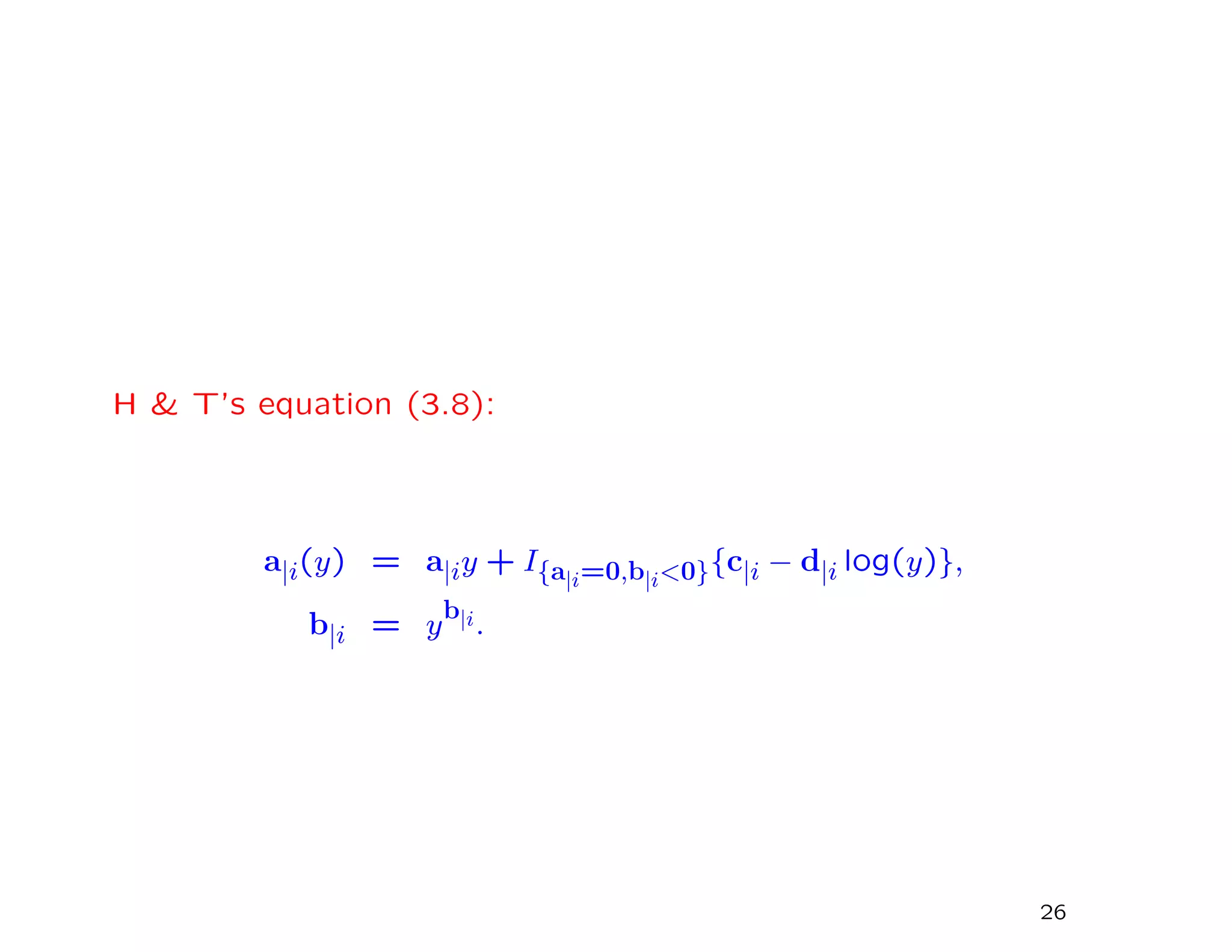
H & T’s equation (3.8):
a|i(y) = a|iy + I{a|i=0,b|i<0}{c|i − d|i log(y)},
b|i = y
b|i.
26
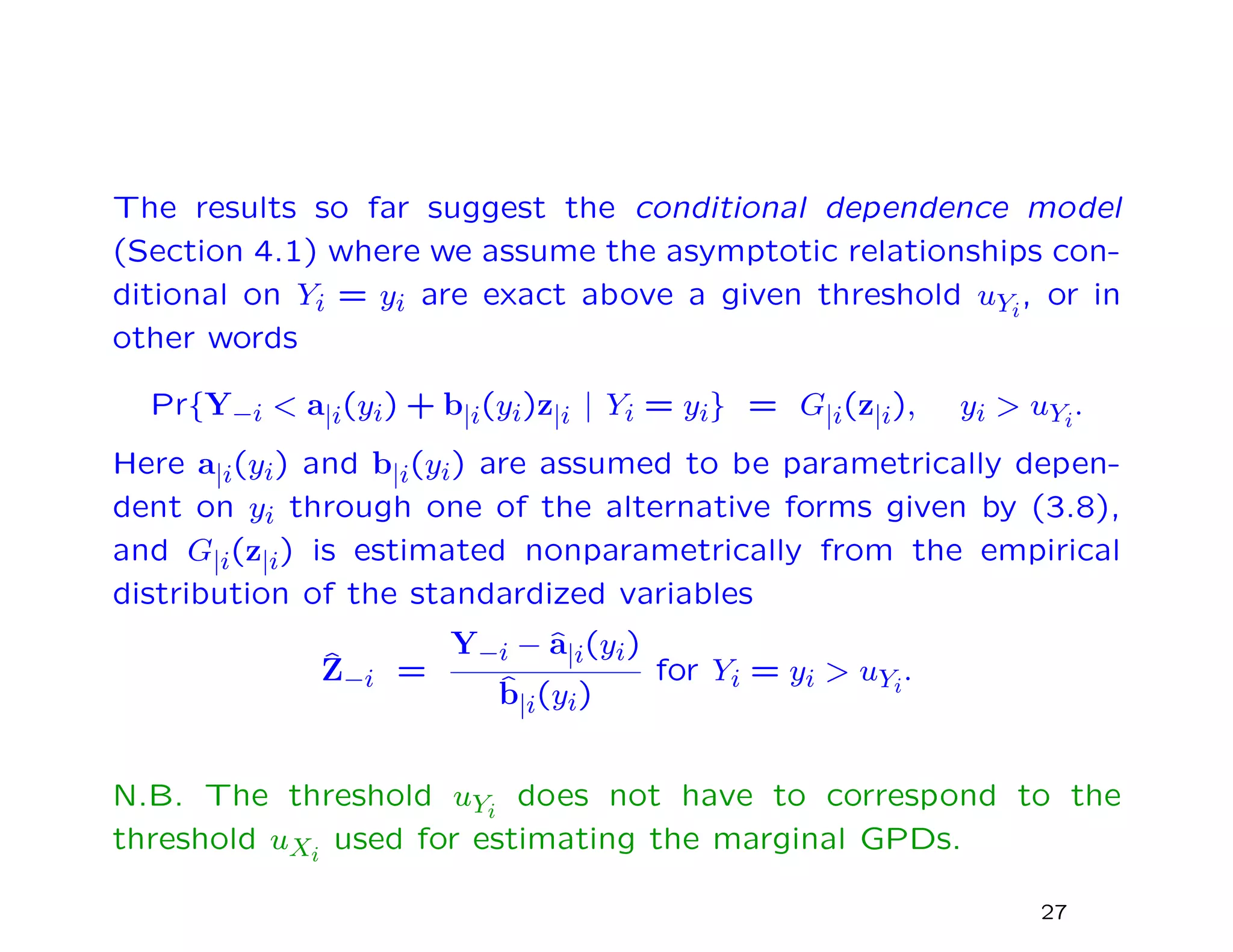
The results so far suggest the conditional dependence model
(Section 4.1) where we assume the asymptotic relationships con-
ditional on Yi = yi are exact above a given threshold uYi
, or in
other words
Pr{Y−i < a|i(yi) + b|i(yi)z|i | Yi = yi} = G|i(z|i), yi > uYi
.
Here a|i(yi) and b|i(yi) are assumed to be parametrically depen-
dent on yi through one of the alternative forms given by (3.8),
and G|i(z|i) is estimated nonparametrically from the empirical
distribution of the standardized variables
ˆZ−i =
Y−i − ˆa|i(yi)
ˆb|i(yi)
for Yi = yi > uYi
.
N.B. The threshold uYi
does not have to correspond to the
threshold uXi
used for estimating the marginal GPDs.
27
In the remainder of the paper, they
1. Proposed an estimation method
2. Discussed various issues such as self-consistency of the rep-
resentation, the use of these models for extrapolation, and
diagnostics
3. Presented an example about the joint distribution of air pol-
lutants (daily values of O3, NO2, NO, SO2, PM10 in Leeds,
U.K., during 1994–1998). The objective was to study condi-
tions where at least one of the five pollutants was extreme,
28
III. Spatial Extremes
Presentation follows a forthcoming book chapter by A. Davison,
R. Huser and E. Thibaud, to appear in Handbook of Environ-
mental Statistics, eds. A. Gelfand, M. Fuentes, J. Hoeting and
R. Smith, Chapman and Hall, to appear
29
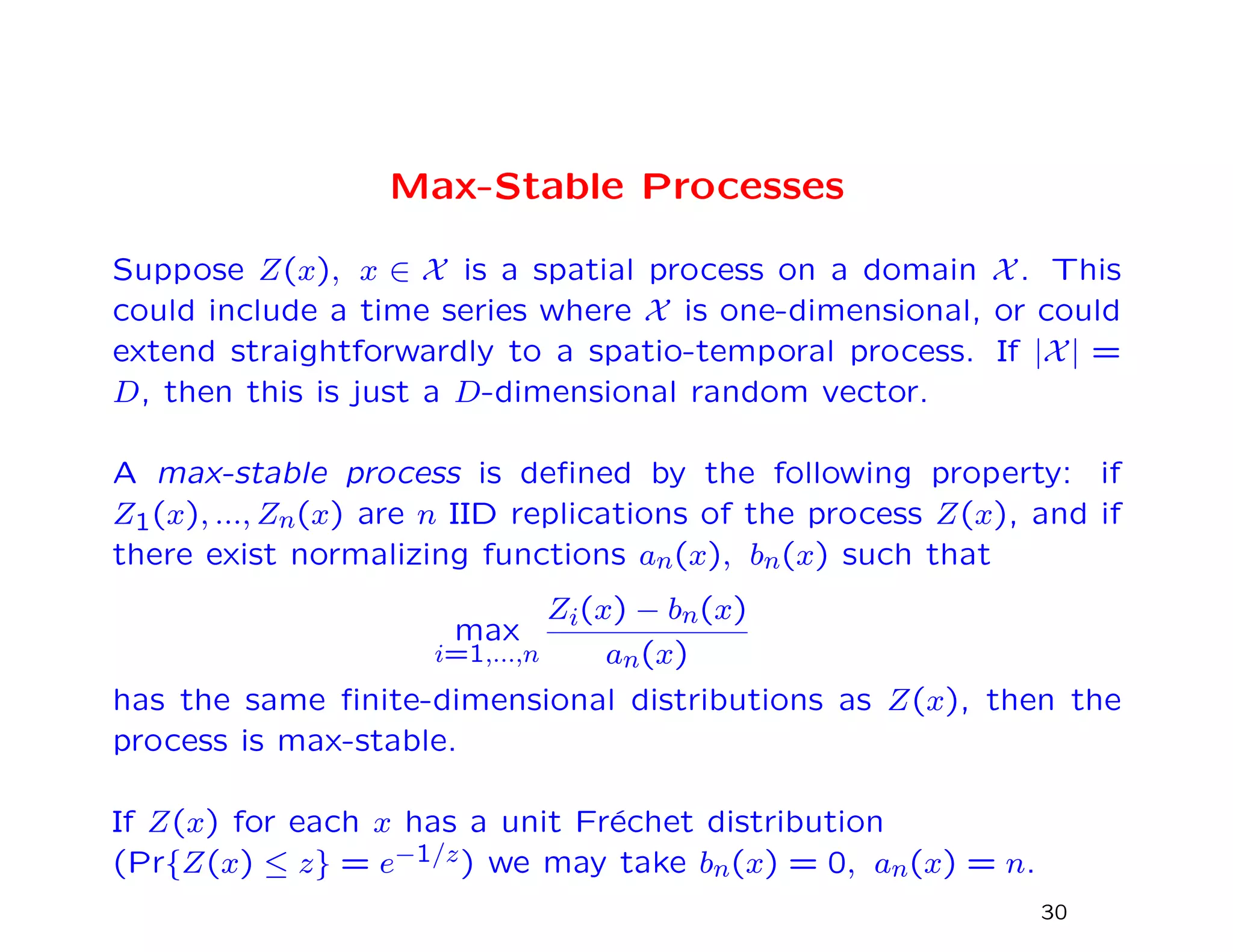
Max-Stable Processes
Suppose Z(x), x ∈ X is a spatial process on a domain X. This
could include a time series where X is one-dimensional, or could
extend straightforwardly to a spatio-temporal process. If |X| =
D, then this is just a D-dimensional random vector.
A max-stable process is defined by the following property: if
Z1(x), ..., Zn(x) are n IID replications of the process Z(x), and if
there exist normalizing functions an(x), bn(x) such that
max
i=1,...,n
Zi(x) − bn(x)
an(x)
has the same finite-dimensional distributions as Z(x), then the
process is max-stable.
If Z(x) for each x has a unit Fr´echet distribution
(Pr{Z(x) ≤ z} = e−1/z) we may take bn(x) = 0, an(x) = n.
30
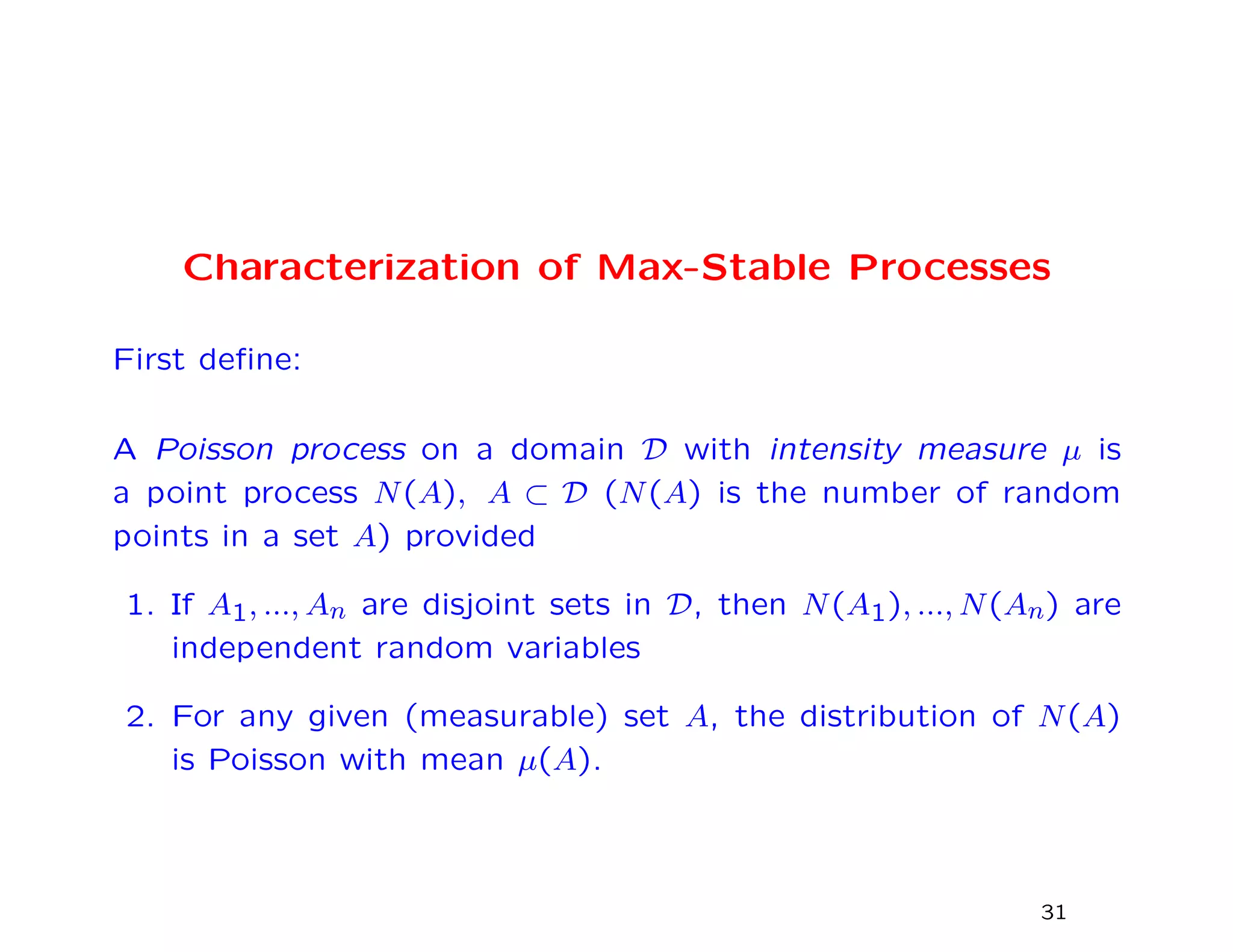
Characterization of Max-Stable Processes
First define:
A Poisson process on a domain D with intensity measure µ is
a point process N(A), A ⊂ D (N(A) is the number of random
points in a set A) provided
1. If A1, ..., An are disjoint sets in D, then N(A1), ..., N(An) are
independent random variables
2. For any given (measurable) set A, the distribution of N(A)
is Poisson with mean µ(A).
31
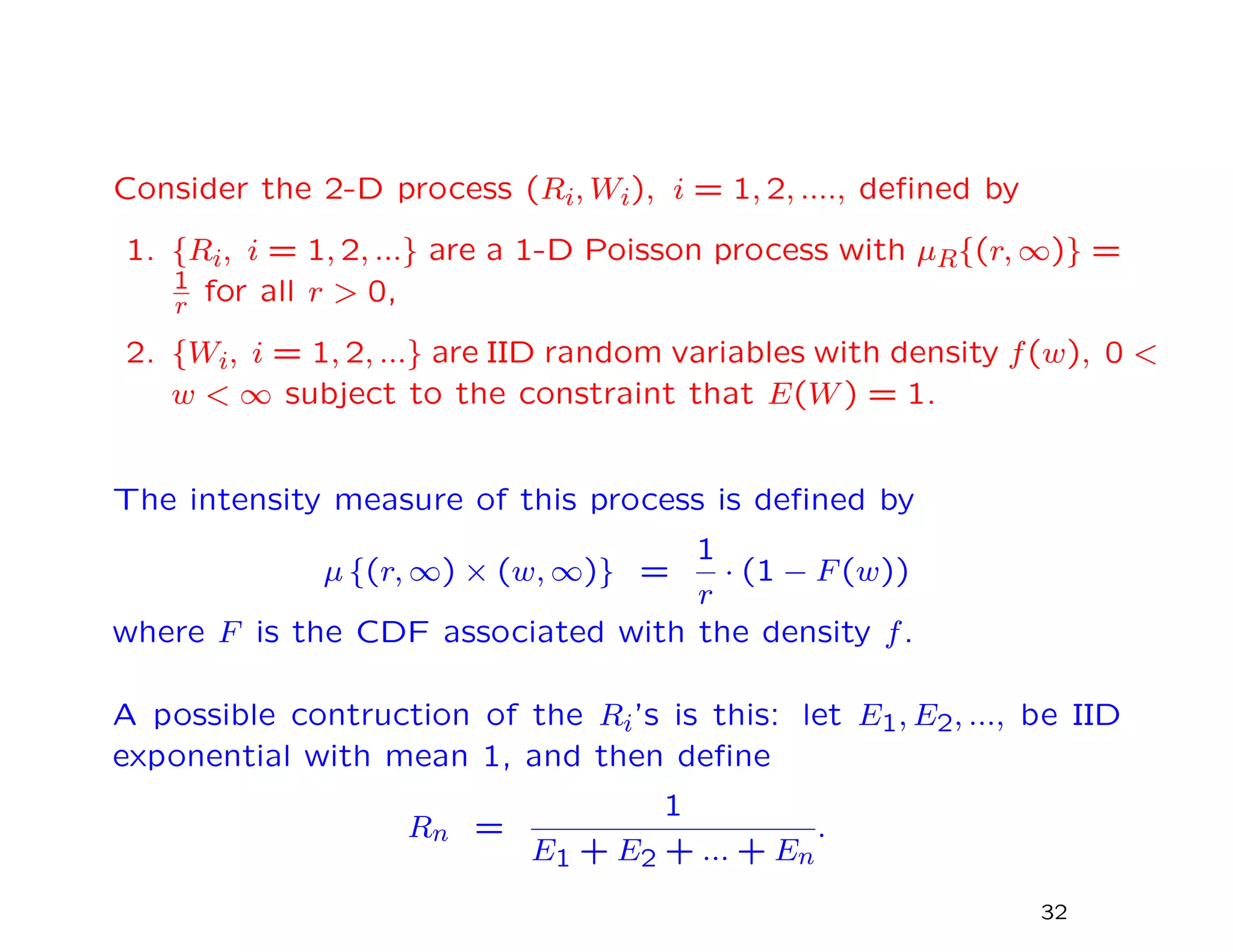
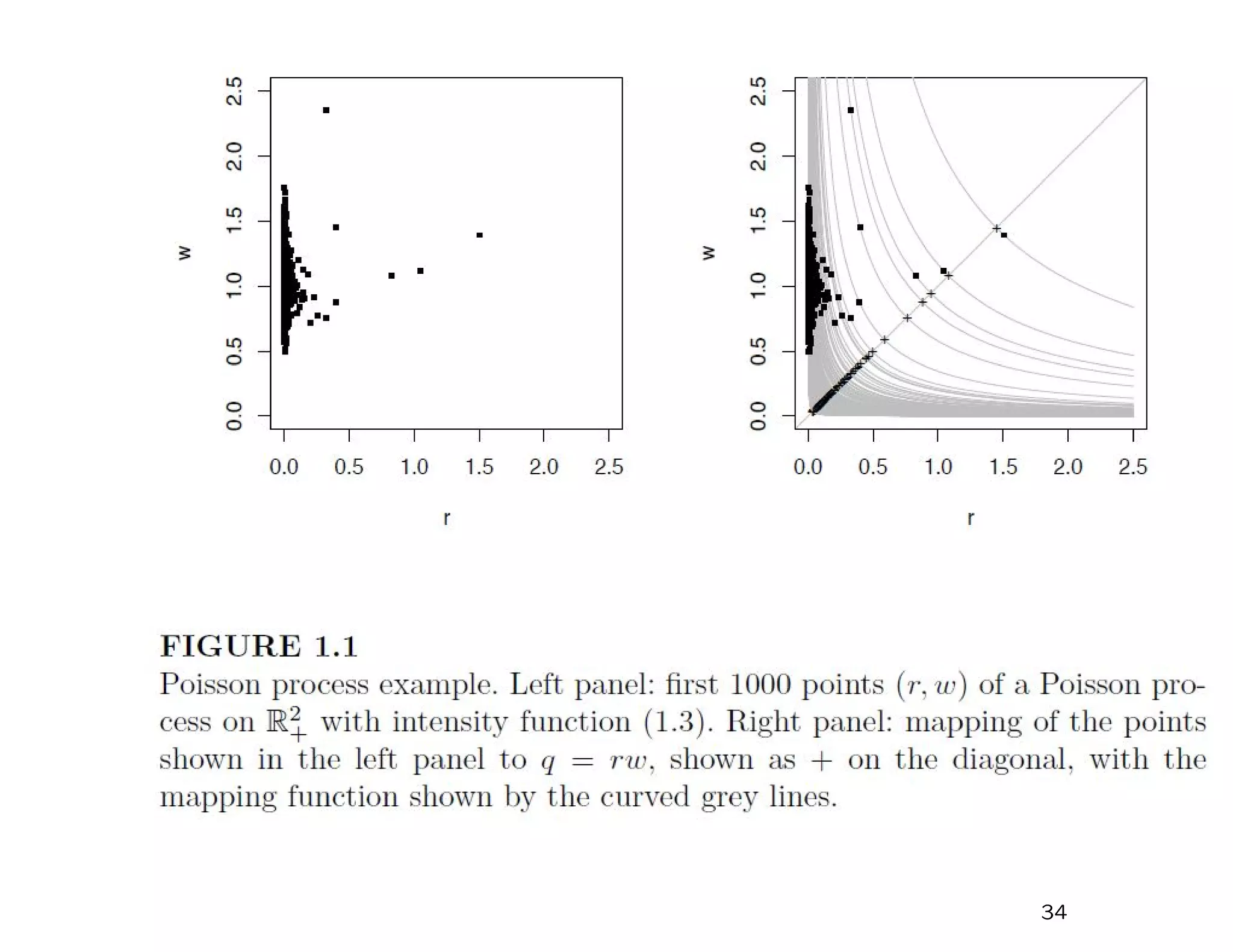
Consider the 2-D process (Ri, Wi), i = 1, 2, ...., defined by
1. {Ri, i = 1, 2, ...} are a 1-D Poisson process with µR{(r, ∞)} =
1
r for all r > 0,
2. {Wi, i = 1, 2, ...} are IID random variables with density f(w), 0 <
w < ∞ subject to the constraint that E(W) = 1.
The intensity measure of this process is defined by
µ {(r, ∞) × (w, ∞)} =
1
r
· (1 − F(w))
where F is the CDF associated with the density f.
A possible contruction of the Ri’s is this: let E1, E2, ..., be IID
exponential with mean 1, and then define
Rn =
1
E1 + E2 + ... + En
.
32
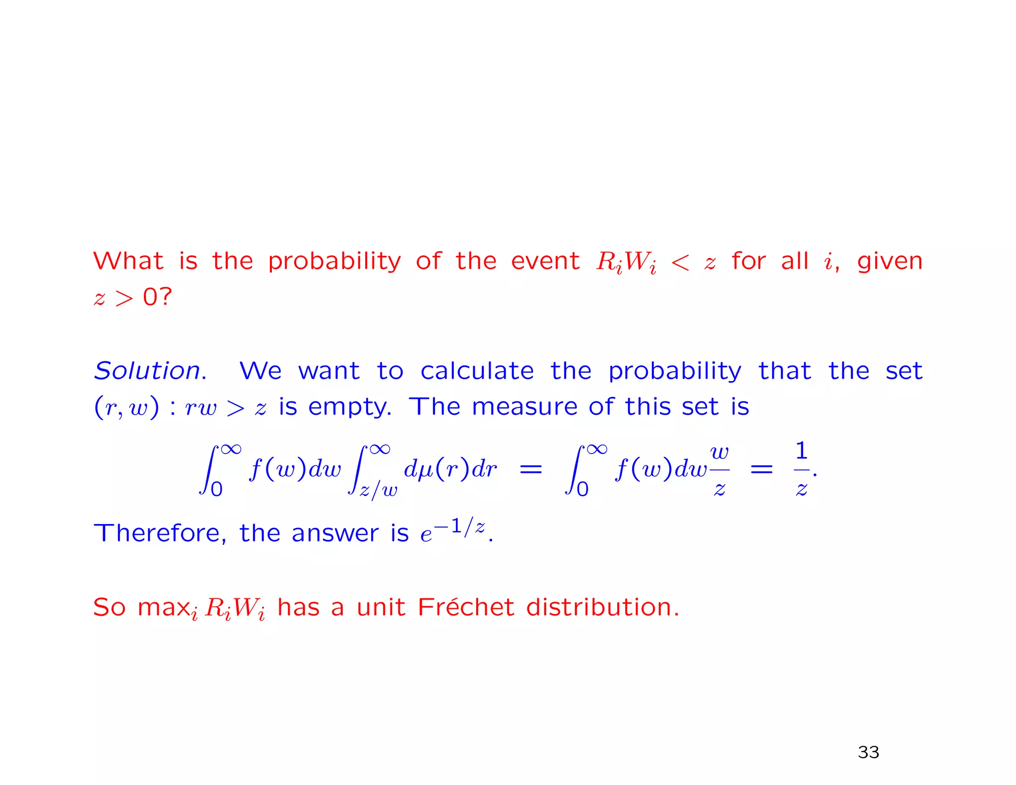
What is the probability of the event RiWi < z for all i, given
z > 0?
Solution. We want to calculate the probability that the set
(r, w) : rw > z is empty. The measure of this set is
∞
0
f(w)dw
∞
z/w
dµ(r)dr =
∞
0
f(w)dw
w
z
=
1
z
.
Therefore, the answer is e−1/z.
So maxi RiWi has a unit Fr´echet distribution.
33
Heffernan and Tawn (2004)
34
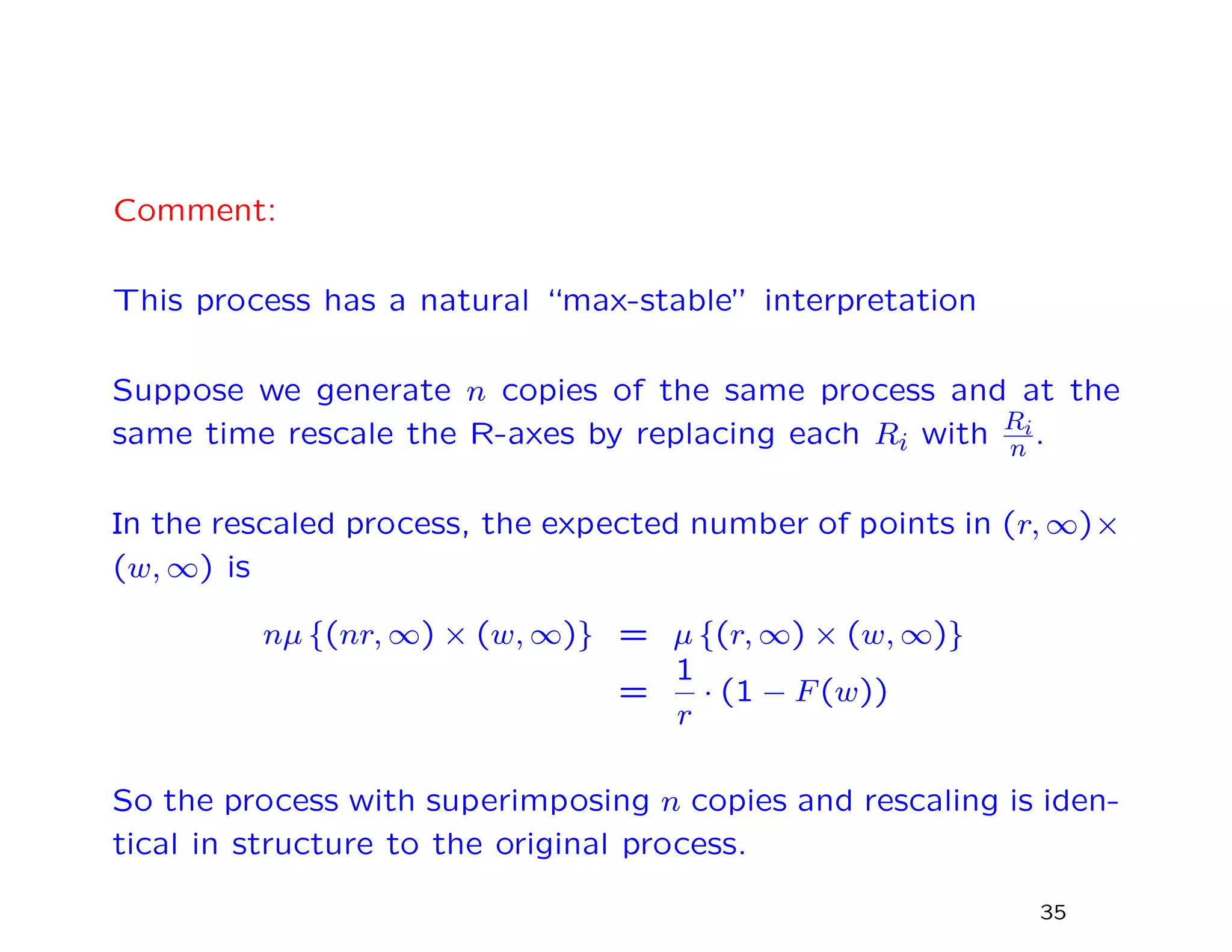
Comment:
This process has a natural “max-stable” interpretation
Suppose we generate n copies of the same process and at the
same time rescale the R-axes by replacing each Ri with Ri
n .
In the rescaled process, the expected number of points in (r, ∞)×
(w, ∞) is
nµ {(nr, ∞) × (w, ∞)} = µ {(r, ∞) × (w, ∞)}
=
1
r
· (1 − F(w))
So the process with superimposing n copies and rescaling is iden-
tical in structure to the original process.
35
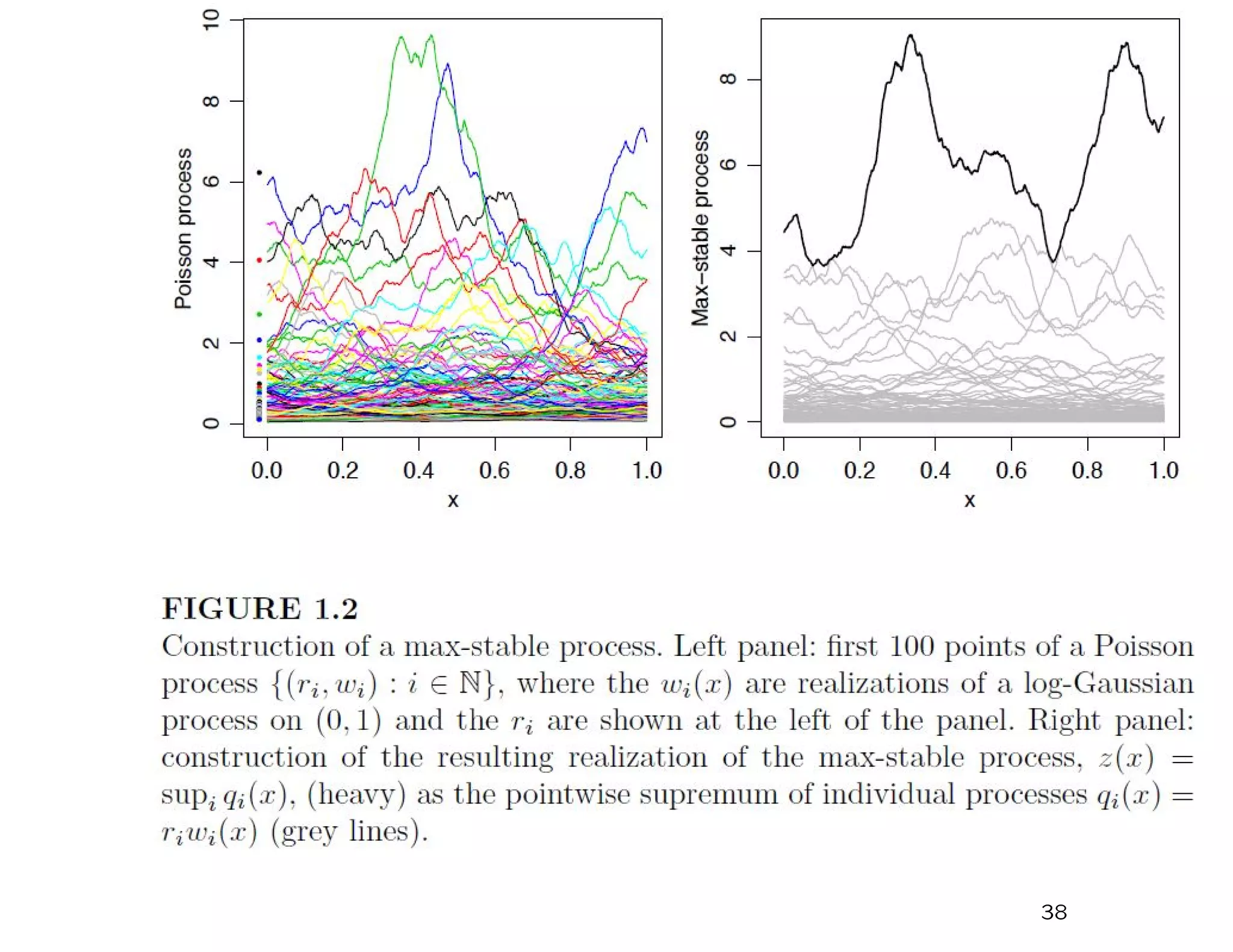
Now consider a process (Ri, Wi(x)), i = 1, 2, ...., x ∈ D:
1. {Ri, i = 1, 2, ...} Poisson process with µ{(r, ∞)} = 1
r , r > 0,
2. {Wi(x), i = 1, 2, ...} IID random processes s.t. E{W(x)} = 1
for all x ∈ D.
An example of such a process would be W(x) = exp{σε(x) − σ2/2} with
σ > 0, ε(·) a stationary Gaussian process with mean 0, variance 1.
What is the probability of the event RiWi(x) < z(x) for all i =
1, 2, ..., x ∈ X, given a function z(x), x ∈ X?
In (R, W) space, the following set must be empty:
R > inf
x∈X
z(x)
W(x)
.
The measure of this set is
V {z(x), x ∈ X} = E sup
x∈X
W(x)
z(x)
.
Therefore,
Pr{RiWi(x) < z(x), i = 1, 2, ..., x ∈ X} = exp [−V {z(x), x ∈ X}] .
36
Note that V is homogeneous of order –1:
V {az(x), x ∈ X} =
1
a
V {z(x), x ∈ X}, a > 0
Define the process Z(x) = maxi=1,2,... RiWi(x) where Ri and Wi
are defined as previously.
If Z1(x), ..., Zn(x) are IID copies of this process then
Pr {Z1(x) ≤ z(x), ..., Zn(x) ≤ z(x) for all x ∈ X}
xxxxxxx = Prn {Z1(x) ≤ z(x) for all x ∈ X}
xxxxxxx = exp [−nV {z(x), x ∈ X}]
xxxxxxx = exp −V
z(x)
n
, x ∈ X
so the process Z(x), x ∈ D is max-stable.
37
Heffernan and Tawn (2004)
38
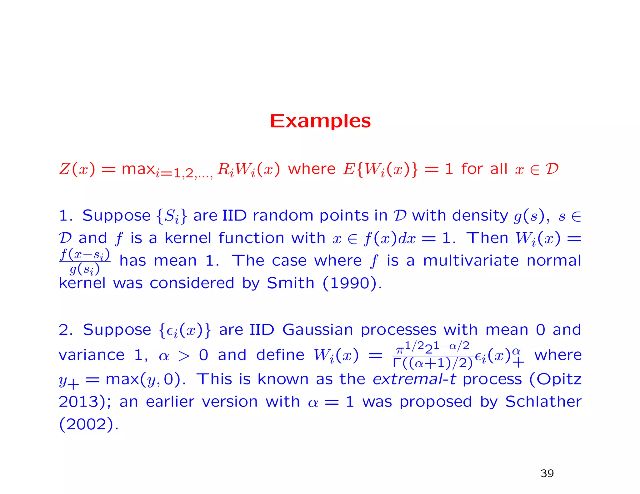
Examples
Z(x) = maxi=1,2,..., RiWi(x) where E{Wi(x)} = 1 for all x ∈ D
1. Suppose {Si} are IID random points in D with density g(s), s ∈
D and f is a kernel function with x ∈ f(x)dx = 1. Then Wi(x) =
f(x−si)
g(si)
has mean 1. The case where f is a multivariate normal
kernel was considered by Smith (1990).
2. Suppose { i(x)} are IID Gaussian processes with mean 0 and
variance 1, α > 0 and define Wi(x) = π1/221−α/2
Γ((α+1)/2) i(x)α
+ where
y+ = max(y, 0). This is known as the extremal-t process (Opitz
2013); an earlier version with α = 1 was proposed by Schlather
(2002).
39
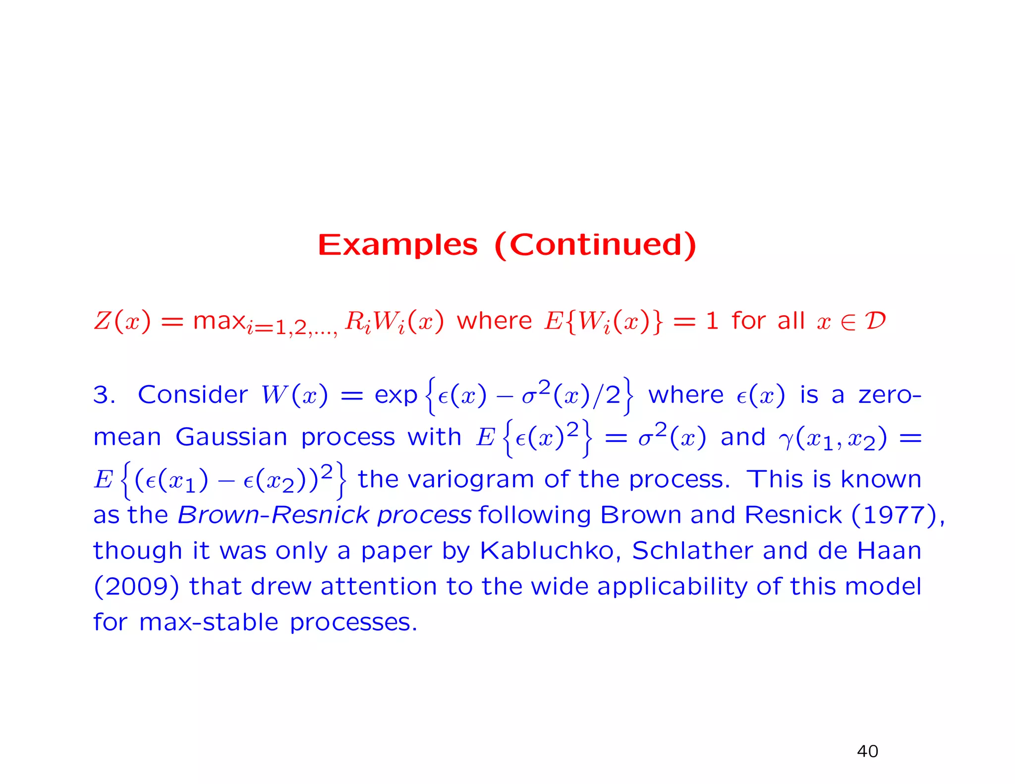
Examples (Continued)
Z(x) = maxi=1,2,..., RiWi(x) where E{Wi(x)} = 1 for all x ∈ D
3. Consider W(x) = exp (x) − σ2(x)/2 where (x) is a zero-
mean Gaussian process with E (x)2 = σ2(x) and γ(x1, x2) =
E ( (x1) − (x2))2 the variogram of the process. This is known
as the Brown-Resnick process following Brown and Resnick (1977),
though it was only a paper by Kabluchko, Schlather and de Haan
(2009) that drew attention to the wide applicability of this model
for max-stable processes.
40
An Issue with the Brown-Resnick Process
It’s possible to calculate the bivariate distributions analytically:
Pr {Z(x1) ≤ z1, Z(x2) ≤ z2} =
exp −
1
z1
Φ
a
2
+
1
a
log
z2
z1
−
1
z2
Φ
a
2
+
1
a
log
z1
z2
where Φ is the standard normal CDF and a = γ(x1, x2). In
particular, when z1 = z2 = z, this reduces to
Pr {Z(x1) ≤ z, Z(x2) ≤ z} = exp −
2
z
Φ
1
2
γ(x1, x2)
However, it’s natural to expect asymptotic independence as x1 − x2 → ∞
and this is only true if γ(x1, x2) → ∞. Therefore, the processes that are of
most interest are those that are intrinsically stationary but not stationary. A
common choice is γ(x1, x2) = ||x1−x2||
λ
κ
with 0 < κ < 2. This is in preference
to common spatial covariance functions such as exponential and Mat´ern.
41
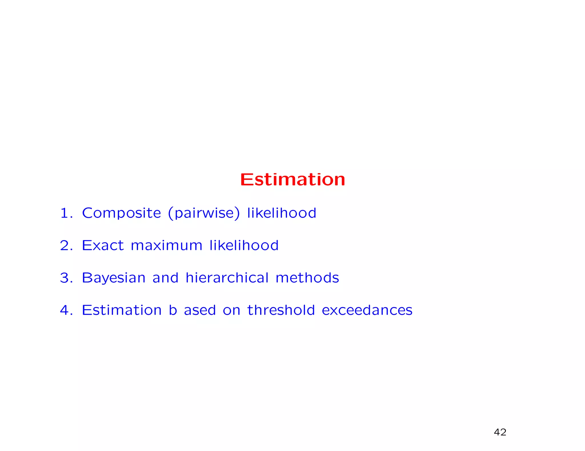
Estimation
1. Composite (pairwise) likelihood
2. Exact maximum likelihood
3. Bayesian and hierarchical methods
4. Estimation b ased on threshold exceedances
42
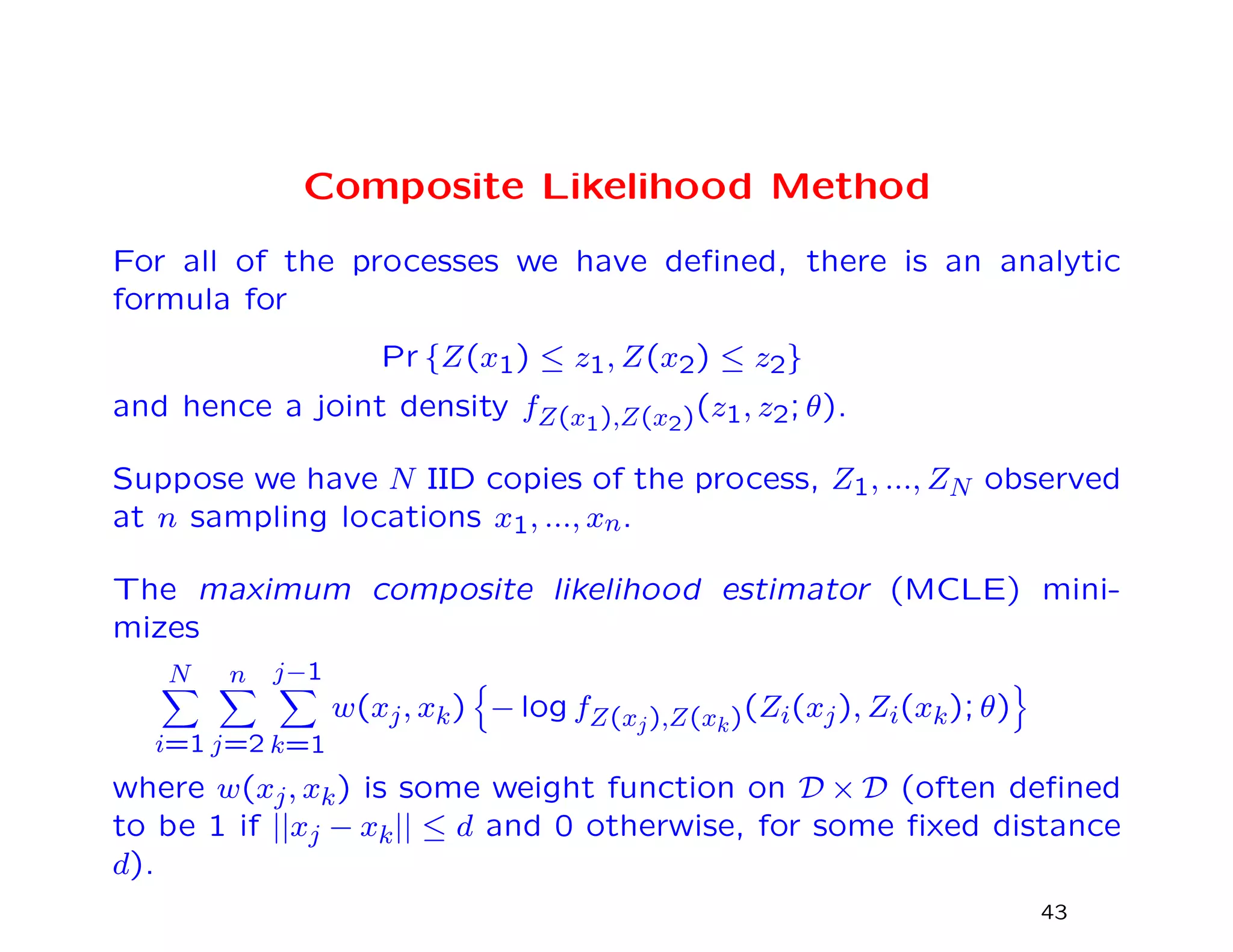
Composite Likelihood Method
For all of the processes we have defined, there is an analytic
formula for
Pr {Z(x1) ≤ z1, Z(x2) ≤ z2}
and hence a joint density fZ(x1),Z(x2)(z1, z2; θ).
Suppose we have N IID copies of the process, Z1, ..., ZN observed
at n sampling locations x1, ..., xn.
The maximum composite likelihood estimator (MCLE) mini-
mizes
N
i=1
n
j=2
j−1
k=1
w(xj, xk) − log fZ(xj),Z(xk)(Zi(xj), Zi(xk); θ)
where w(xj, xk) is some weight function on D × D (often defined
to be 1 if ||xj − xk|| ≤ d and 0 otherwise, for some fixed distance
d).
43
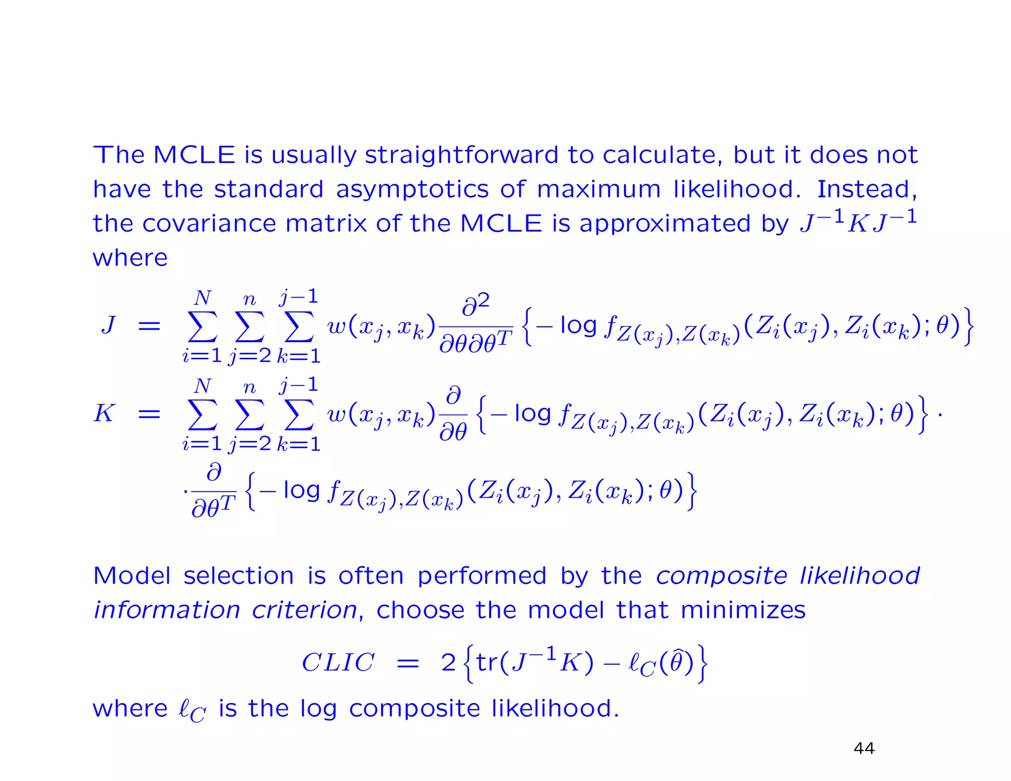
The MCLE is usually straightforward to calculate, but it does not
have the standard asymptotics of maximum likelihood. Instead,
the covariance matrix of the MCLE is approximated by J−1KJ−1
where
J =
N
i=1
n
j=2
j−1
k=1
w(xj, xk)
∂2
∂θ∂θT
− log fZ(xj),Z(xk)(Zi(xj), Zi(xk); θ)
K =
N
i=1
n
j=2
j−1
k=1
w(xj, xk)
∂
∂θ
− log fZ(xj),Z(xk)(Zi(xj), Zi(xk); θ) ·
·
∂
∂θT
− log fZ(xj),Z(xk)(Zi(xj), Zi(xk); θ)
Model selection is often performed by the composite likelihood
information criterion, choose the model that minimizes
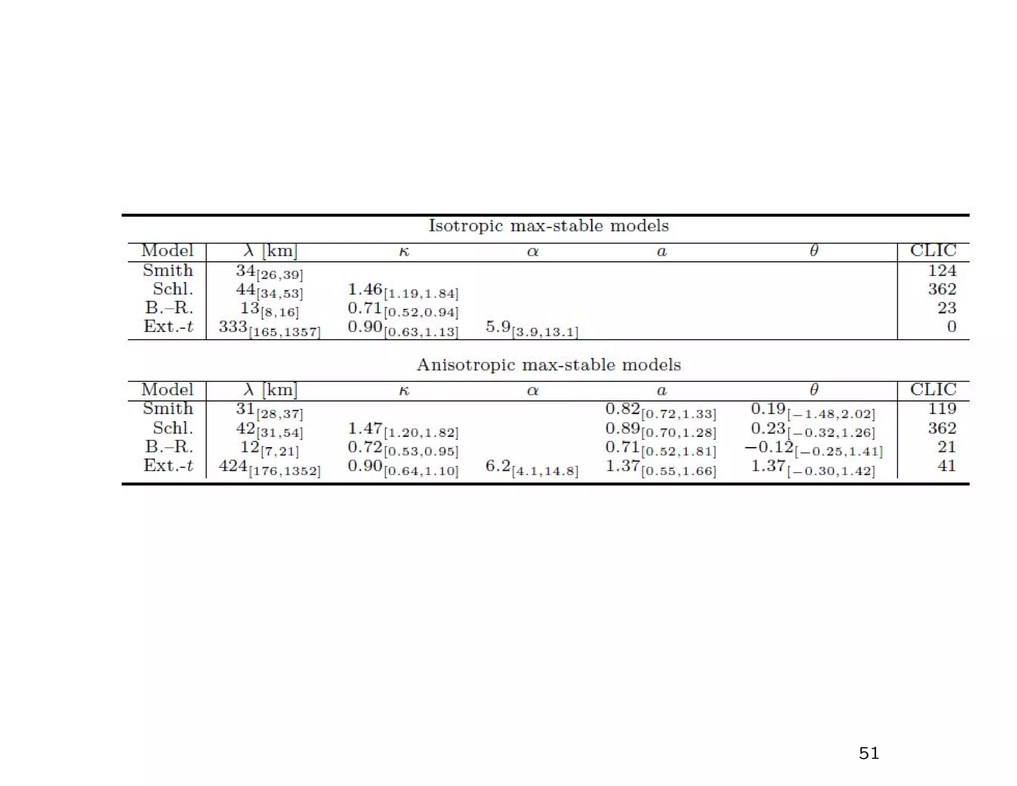
CLIC = 2 tr(J−1K) − C(ˆθ)
where C is the log composite likelihood.
44
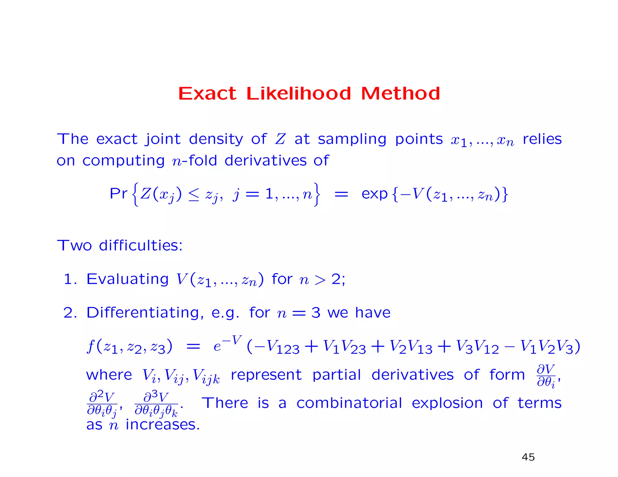
Exact Likelihood Method
The exact joint density of Z at sampling points x1, ..., xn relies
on computing n-fold derivatives of
Pr Z(xj) ≤ zj, j = 1, ..., n = exp {−V (z1, ..., zn)}
Two difficulties:
1. Evaluating V (z1, ..., zn) for n > 2;
2. Differentiating, e.g. for n = 3 we have
f(z1, z2, z3) = e−V
(−V123 + V1V23 + V2V13 + V3V12 − V1V2V3)
where Vi, Vij, Vijk represent partial derivatives of form ∂V
∂θi
,
∂2V
∂θiθj
, ∂3V
∂θiθjθk
. There is a combinatorial explosion of terms
as n increases.
45
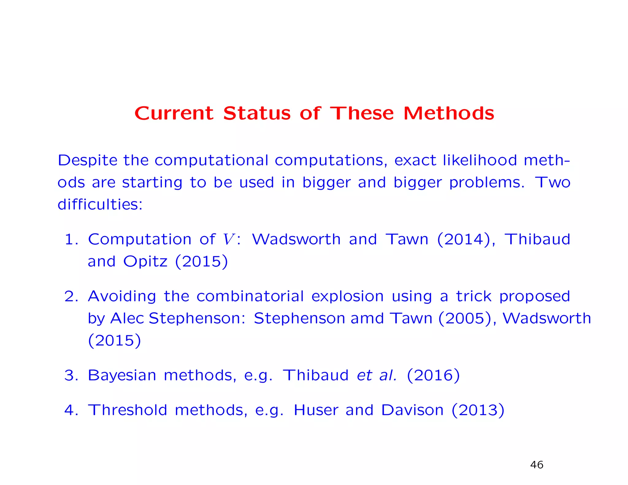
Current Status of These Methods
Despite the computational computations, exact likelihood meth-
ods are starting to be used in bigger and bigger problems. Two
difficulties:
1. Computation of V : Wadsworth and Tawn (2014), Thibaud
and Opitz (2015)
2. Avoiding the combinatorial explosion using a trick proposed
by Alec Stephenson: Stephenson amd Tawn (2005), Wadsworth
(2015)
3. Bayesian methods, e.g. Thibaud et al. (2016)
4. Threshold methods, e.g. Huser and Davison (2013)
46
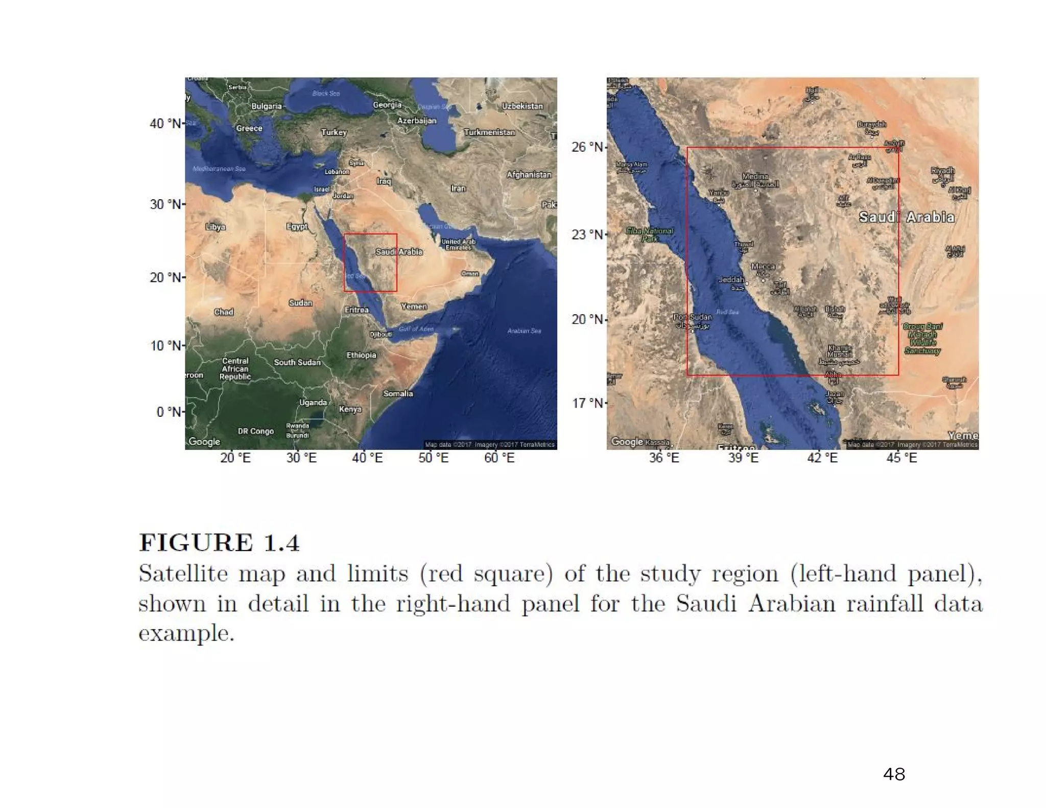
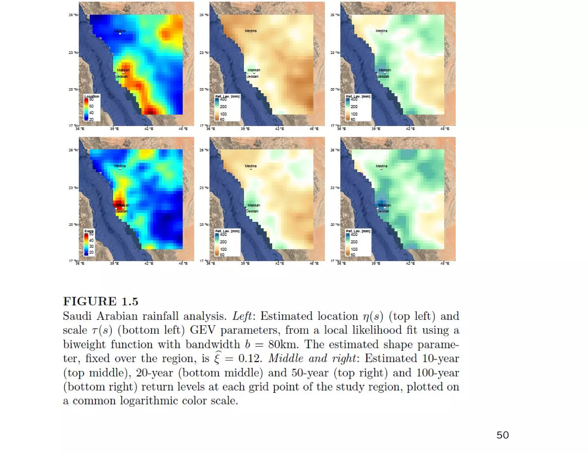
An Example
(Davison, Huser and Thibaud, 2018)
Data from Saudi Arabia: 17 annual maxima at each of 750 1
4-
degree grid boxes
Objective to understand spatial clustering of sever storms near
Jeddah
47
Heffernan and Tawn (2004)
48
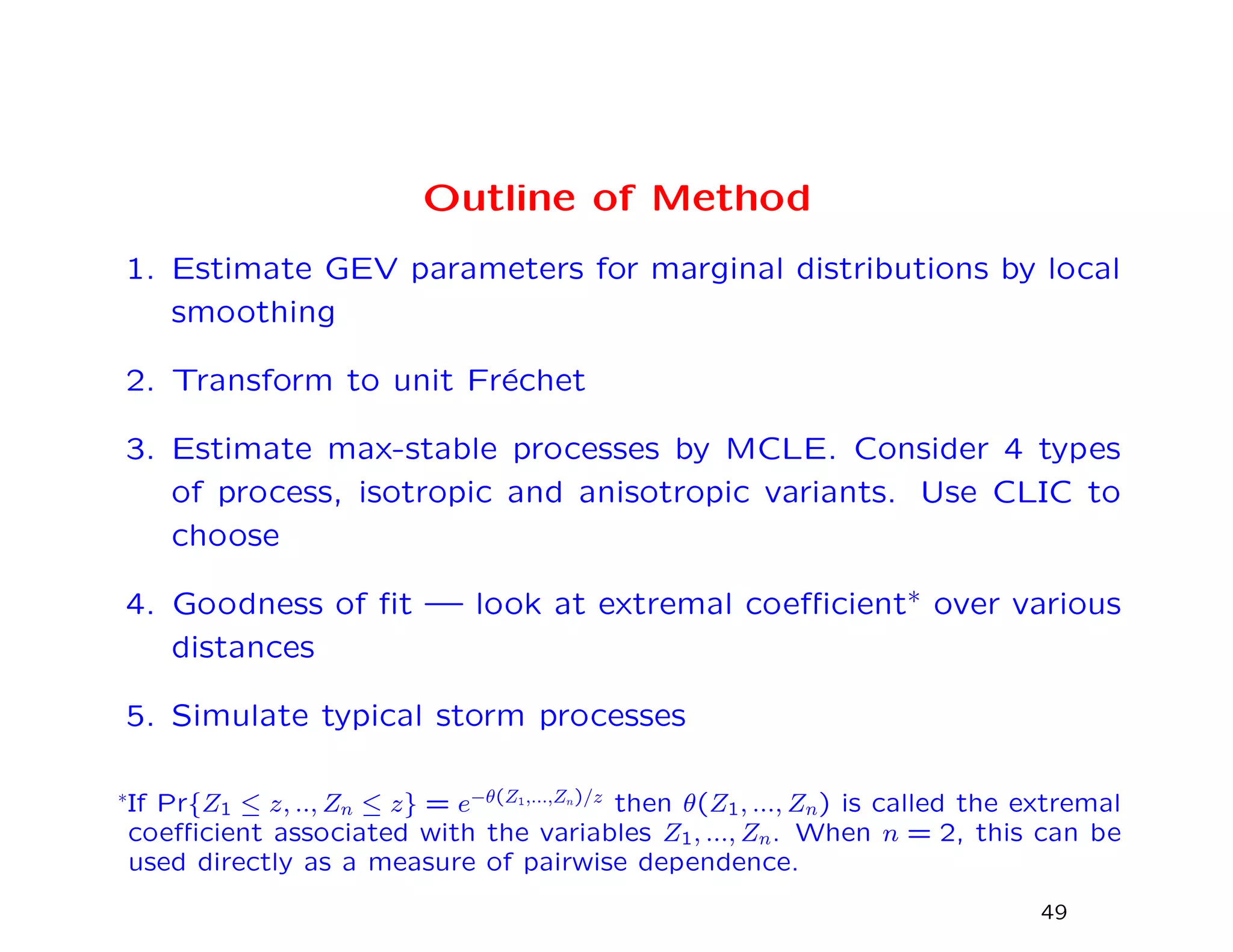
Outline of Method
1. Estimate GEV parameters for marginal distributions by local
smoothing
2. Transform to unit Fr´echet
3. Estimate max-stable processes by MCLE. Consider 4 types
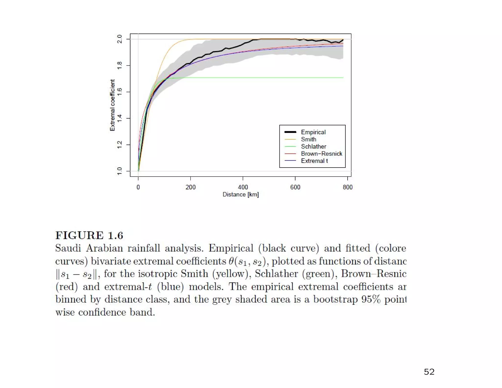
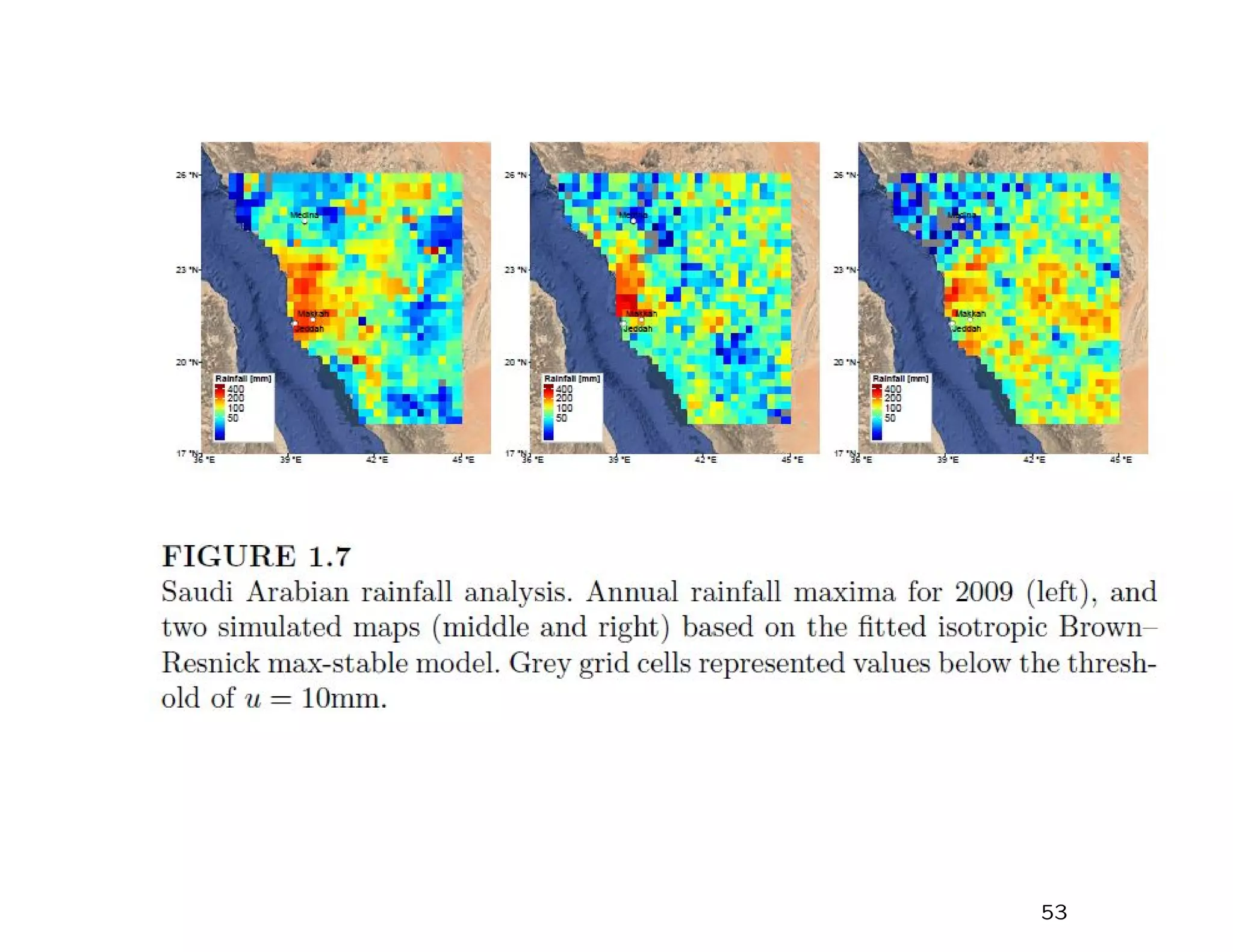
of process, isotropic and anisotropic variants. Use CLIC to
choose
4. Goodness of fit — look at extremal coefficient∗ over various
distances
5. Simulate typical storm processes
∗If Pr{Z1 ≤ z, .., Zn ≤ z} = e−θ(Z1,...,Zn)/z then θ(Z1, ..., Zn) is called the extremal
coefficient associated with the variables Z1, ..., Zn. When n = 2, this can be
used directly as a measure of pairwise dependence.
49
Heffernan and Tawn (2004)
50
Heffernan and Tawn (2004)
51
Heffernan and Tawn (2004)
52
Heffernan and Tawn (2004)
53
Conclusions
1. Bivariate extreme value theory is now very well established.
For further examples, see the book chapter by D. Coo-
ley, B.D. Hunter and R. Smith, Univariate and Multivari-
ate Extremes for the Environmental Sciences, to appear in
Handbook of Environmental Statistics, eds. A. Gelfand, M.
Fuentes, J. Hoeting and R. Smith, Chapman and Hall, to
appear
2. The alternative formulation initiated by Ledford and Tawn is
also widely used — important distinction between asymptot-
ically dependent and asymptotically independent
3. However, some of this is stll a stretch for dimensions d > 2!
4. An alternative formulation is the Heffernan-Tawn approach
5. Spatial extremes based on max-stable processes is a very
active area of research
6. Still scope for altrnative formulations of spatial extremes!
54

CLIM Fall 2017 Course: Statistics for Climate Research, Statistics of Climate Extremes: Multivariate & Spacial Extremes - Richard Smith, Nov 28, 2017

  • 1.
    STATISTICS OF CLIMATEEXTREMES: MULTIVARIATE AND SPATIAL EXTREMES Richard L Smith Departments of STOR and Biostatistics, University of North Carolina at Chapel Hill and Statistical and Applied Mathematical Sciences Institute (SAMSI) SAMSI Graduate Class November 28, 2017 1 Heffernan and Tawn (2004) 1
  • 2.
    MULTIVARIATE EXTREMES AND MAX-STABLEPROCESSES I Limit theory for multivariate sample maxima II Alternative formulations of multivariate extreme value theory III Max-stable processes 2
  • 3.
    Multivariate extreme valuetheory applies when we are interested in the joint distribution of extremes from several random vari- ables. Examples: • Winds and waves on an offshore structure • Meteorological variables, e.g. temperature and precipitation • Air pollution variables, e.g. ozone and sulfur dioxide • Finance, e.g. price changes in several stocks or indices • Spatial extremes, e.g. joint distributions of extreme precipi- tation at several locations 3
  • 4.
    I LIMIT THEOREMSFOR MULTIVARIATE SAMPLE MAXIMA Let Yi = (Yi1...YiD)T be i.i.d. D-dimensional vectors, i = 1, 2, ... Mnd = max{Y1d, ..., Ynd}(1 ≤ d ≤ D) — d’th-component maxi- mum Look for constants and, bnd such that Pr Mnd − bnd and ≤ xd, d = 1, ..., D → G(x1, ..., xD). Vector notation: Pr Mn − bn an ≤ x → G(x). 4
  • 5.
    Two general points: 1.If G is a multivariate extreme value distribution, then each of its marginal distributions must be one of the univariate extreme value distributions, and therefore can be represented in GEV form 2. The form of the limiting distribution is invariant under mono- tonic transformation of each component. Therefore, without loss of generality we can transform each marginal distribu- tion into a specified form. For most of our applications, it is convenient to assume the Fr´echet form: Pr{Xd ≤ x} = exp(−x−α), x > 0, d = 1, ..., D. Here α > 0. The case α = 1 is called unit Fr´echet. 5
  • 6.
    Representations of LimitDistributions Any MEVD with unit Fr´echet margins may be written as G(x) = exp {−V (x)} , (1) V (x) = SD max d=1,...,D wj xj dH(w), (2) where SD = {(x1, ..., xD) : x1 ≥ 0, ..., xD ≥ 0, x1 + ... + xD = 1} and H is a measure on SD. The function V (x) is called the exponent measure and formula (2) is the Pickands representation. If we fix d ∈ {1, ..., D} with 0 < xd < ∞, and define xd = +∞ for d = d , then V (x) = SD max d=1,...,D wd xd dH(w) = 1 xd SD wd dH(w) so to ensure correct marginal distributions we must have SD wddH(w) = 1, d = 1, ..., D. (3) 6
  • 7.
    Note that kV (x)= V x k (which is in fact another characterization of V ) so Gk(x) = exp(−kV (x)) = exp −V x k = G x k . Hence G is max-stable. In particular, if X1, ..., Xk are i.i.d. from G, then max{X1, ..., Xk} (vector of componentwise maxima) has the same distribution as kX1. 7
  • 8.
    The Pickands DependenceFunction In the two-dimensional case (with unit Fr´echet margins) there is an alternative representation due to Pickands: Pr{X1 ≤ x1, X2 ≤ x2} = exp − 1 x1 + 1 x2 A x1 x1 + x2 where A is a convex function on [0,1] such that A(0) = A(1) = 1, 1 2 ≤ A 1 2 ≤ 1. The value of A 1 2 is often taken as a measure of the strength of dependence: A 1 2 = 1 2 is “perfect dependence” while A 1 2 = 1 is independence. 8
  • 9.
  • 10.
    Logistic (Gumbel andGoldstein, 1964) V (x) =   D d=1 x−r d   1/r , r ≥ 1. Check: 1. V (x/k) = kV (x) 2. V ((+∞, +∞, ..., xd, ..., +∞, +∞) = x−1 d 3. e−V (x) is a valid c.d.f. Limiting cases: • r = 1: independent components • r → ∞: the limiting case when Xi1 = Xi2 = ... = XiD with probability 1. 10
  • 11.
    Asymmetric logistic (Tawn1990) V (x) = c∈C    i∈c θi,c xi rc    1/rc , where C is the class of non-empty subsets of {1, ..., D}, rc ≥ 1, θi,c = 0 if i /∈ c, θi,c ≥ 0, c∈C θi,c = 1 for each i. Negative logistic (Joe 1990) V (x) = 1 xj + c∈C: |c|≥2 (−1)|c|    i∈c θi,c xi rc    1/rc , rc ≤ 0, θi,c = 0 if i /∈ c, θi,c ≥ 0, c∈C(−1)|c|θi,c ≤ 1 for each i. 11
  • 12.
    Tilted Dirichlet (Colesand Tawn 1991) A general construction: Suppose h∗ is an arbitrary positive func- tion on Sd with md = SD udh∗(u)du < ∞, then define h(w) = ( mkwk)−(D+1) D d=1 mdh∗ m1w1 mkwk , ..., mDwD mkwk . h is density of positive measure H, SD uddH(u) = 1 each d. As a special case of this, they considered Dirichlet density h∗(u) = Γ( αj) d Γ(αd) D d=1 u αd−1 d . Leads to h(w) = D d=1 αd Γ(αd) · Γ( αd + 1) ( αdwd)D+1 D d=1 αdwd αkwk αd−1 . Disadvantage: need for numerical integration 12
  • 13.
    I.b ESTIMATION • Parametric •Non/semi-parametric Both approaches have problems, e.g. nonregular behavior of MLE even in finite-parameter problems; curse of dimensionality if D large. Typically proceed by transforming margins to unit Fr´echet first, though there are advantages in joint estimation of marginal dis- tributions and dependence structure (Shi 1995) 13
  • 14.
    II ALTERNATIVE FORMULATIONSOF MULTIVARIATE EXTREMES 14
  • 15.
    • Ledford-Tawn-Ramos approach •Heffernan-Tawn approach 15
  • 16.
    The first paperto suggest that multivariate extreme value theory (as defined so far) might not be general enough was Ledford and Tawn (1996). Suppose (Z1, Z2) are a bivariate random vector with unit Fr´echet margins. Traditional cases lead to Pr{Z1 > r, Z2 > r} ∼ const. × r−1 dependent cases const. × r−2 exact independent The first case covers all bivariate extreme value distributions ex- cept the independent case. However, Ledford and Tawn showed by example that for a number of cases of practical interest, Pr{Z1 > r, Z2 > r} ∼ L(r)r−1/η, where L is a slowly varying function (L(rx) L(r) → 1 as r → ∞) and η ∈ (0, 1]. Estimation: used fact that 1/η is Pareto index for min(Z1, Z2). 16
  • 17.
    More general case(Ledford and Tawn 1997): Pr{Z1 > z1, Z2 > z2, } = L(z1, z2)z −c1 1 z −c2 2 , 0 < η ≤ 1; c1 + c2 = 1 η; L slowly varying in sense that g(z1, z2) = lim t→∞ L(tz1, tz2) L(t, t) . They showed g(z1, z2) = g∗ z1 z1+z2 but were unable to estimate g∗ directly — needed to make parametric assumptions about this. More recently, Resnick and co-authors were able to make a more rigorous mathematical theory using concept of hidden regular variation (see e.g. Resnick 2002, Maulik and Resnick 2005, Heffernan and Resnick 2005; see also Section 9.4 of Resnick (2007)). 17
  • 18.
    Ramos-Ledford (2009, 2008)approach: Pr{Z1 > z1, Z2 > z2, } = ˜L(z1, z2)(z1z2)−1/(2η), lim u→∞ ˜L(ux1, ux2) ˜L(u, u) = g(x1, x2) = g∗ x1 x1 + x2 Limiting joint survivor function Pr{X1 > x1, X2 > x2} = 1 0 η min w x1 , 1 − w x2 1/η dH∗ η(w), 1 = η 1 0 {min (w, 1 − w)}1/η dH∗ η(w). 18
  • 19.
    Multivariate generalization toD > 2: Pr{X1 > x1, ..., XD > xD} = SD η min 1≤d≤D wd xd 1/η dH∗ η(w), 1 = SD η min 1≤d≤D wj 1/η dH∗ η(w). Open problems: • How to find sufficiently rich classes of H∗ η(w) to derive para- metric families suitable for real data • How to do the subsequent estimation 19
  • 20.
    The Heffernan-Tawn approach Reference: Aconditional approach for multivariate extreme values, by Janet Heffernan and Jonathan Tawn, J.R. Statist. Soc. B 66, 497– 546 (with discussion) 20
  • 21.
    A set C∈ Rd is an “extreme set” if • we can partition C = ∪d i=1Ci where Ci = C ∩ x ∈ Rd : FXi (xi) > FXj (xj) for all i = j (Ci is the set on which Xi is “most extreme” among X1, ..., Xd, extremeness being measured by marginal tail probabilities) • The set Ci satisfies the following property: there exists a vXi such that X ∈ Ci if and only if X ∈ Ci and Xi > vXi . (or: if X = (X1, ..., Xd) ∈ Ci then so is any other X for which Xi is more extreme) The objective of the paper is to propose a general methodology for estimating probabilities of extreme sets. 21
  • 22.
    Marginal distributions • Standard“GPD” model fit: define a threshold uXi and as- sume Pr{Xi > uXi + x | Xi > uXi } = 1 + ξi x βi −1/ξi + for x > 0. • Also estimate FXi (x) by empirical CDF for x < uXi . • Combine together for an estimate ˆFXi (x) across the entire range of x. • Apply componentwise probability integral transform — Yi = − log[− log{ ˆFXi (Xi)}] to have approximately Gumbel margins (i.e. Pr{Yi ≤ yi} ≈ exp(−e−y)). • Henceforth assume marginal distributions are exactly Gumbel and concentrate on dependence among Y1, ..., Yd. 22
  • 23.
    Existing techniques Most existingextreme value methods with Gumbel margins re- duce to Pr{Y ∈ t + A} ≈ e−t/ηY Pr{Y ∈ A} for some ηY ∈ (0, 1]. Ledford-Tawn classification: • ηY = 1 is asymptotic dependence (includes all conventional multivariate extreme value distributions) • 1 d < ηY < 1 — positive extremal dependence • 0 < ηY < 1 d — negative extremal dependence • ηY = 1 d — near extremal independence Disadvantage: doesn’t work for extreme sets that are not simul- taneously extreme in all components 23
  • 24.
    The key assumptionof Heffernan-Tawn Define Y−i to be the vector Y with i’th component omitted. We assume that for each yi, there exist vectors of normalizing constants a|i(yi) and b|i(yi) and a limiting (d − 1)-dimensional CDF G|i such that lim yi→∞ Pr{Y−i ≤ a|i(yi) + b|i(yi)z|i | Yi = yi} = G|i(z|i). (4) Put another way: as ui → ∞ the variables Yi − ui and Z−i = Y−i − a|i(Yi) b|i(Yi) are asymptotically independent, with distributions unit exponen- tial and G|i(z|i). 24
  • 25.
    Examples in cased = 2 Distribution η a(y) b(y) Perfect pos. dependence 1 y 1 Bivariate EVD 1 y 1 Bivariate normal, ρ > 0 1+ρ 2 ρ2y y1/2 Inverted logistic, α ∈ (0, 1] 2−α 0 y1−α Independent 1 2 0 1 Morganstern 1 2 0 1 Bivariate normal, ρ < 0 1+ρ 2 − log(ρ2y) y−1/2 Perfect neg. dependence 0 − log(y) 1 Key observation: in all cases b(y) = yb for some b and a(y) is either 0 or a linear function of y or − log y (for more precise conditions see equation (3.8) of the paper) 25
  • 26.
    H & T’sequation (3.8): a|i(y) = a|iy + I{a|i=0,b|i<0}{c|i − d|i log(y)}, b|i = y b|i. 26
  • 27.
    The results sofar suggest the conditional dependence model (Section 4.1) where we assume the asymptotic relationships con- ditional on Yi = yi are exact above a given threshold uYi , or in other words Pr{Y−i < a|i(yi) + b|i(yi)z|i | Yi = yi} = G|i(z|i), yi > uYi . Here a|i(yi) and b|i(yi) are assumed to be parametrically depen- dent on yi through one of the alternative forms given by (3.8), and G|i(z|i) is estimated nonparametrically from the empirical distribution of the standardized variables ˆZ−i = Y−i − ˆa|i(yi) ˆb|i(yi) for Yi = yi > uYi . N.B. The threshold uYi does not have to correspond to the threshold uXi used for estimating the marginal GPDs. 27
  • 28.
    In the remainderof the paper, they 1. Proposed an estimation method 2. Discussed various issues such as self-consistency of the rep- resentation, the use of these models for extrapolation, and diagnostics 3. Presented an example about the joint distribution of air pol- lutants (daily values of O3, NO2, NO, SO2, PM10 in Leeds, U.K., during 1994–1998). The objective was to study condi- tions where at least one of the five pollutants was extreme, 28
  • 29.
    III. Spatial Extremes Presentationfollows a forthcoming book chapter by A. Davison, R. Huser and E. Thibaud, to appear in Handbook of Environ- mental Statistics, eds. A. Gelfand, M. Fuentes, J. Hoeting and R. Smith, Chapman and Hall, to appear 29
  • 30.
    Max-Stable Processes Suppose Z(x),x ∈ X is a spatial process on a domain X. This could include a time series where X is one-dimensional, or could extend straightforwardly to a spatio-temporal process. If |X| = D, then this is just a D-dimensional random vector. A max-stable process is defined by the following property: if Z1(x), ..., Zn(x) are n IID replications of the process Z(x), and if there exist normalizing functions an(x), bn(x) such that max i=1,...,n Zi(x) − bn(x) an(x) has the same finite-dimensional distributions as Z(x), then the process is max-stable. If Z(x) for each x has a unit Fr´echet distribution (Pr{Z(x) ≤ z} = e−1/z) we may take bn(x) = 0, an(x) = n. 30
  • 31.
    Characterization of Max-StableProcesses First define: A Poisson process on a domain D with intensity measure µ is a point process N(A), A ⊂ D (N(A) is the number of random points in a set A) provided 1. If A1, ..., An are disjoint sets in D, then N(A1), ..., N(An) are independent random variables 2. For any given (measurable) set A, the distribution of N(A) is Poisson with mean µ(A). 31
  • 32.
    Consider the 2-Dprocess (Ri, Wi), i = 1, 2, ...., defined by 1. {Ri, i = 1, 2, ...} are a 1-D Poisson process with µR{(r, ∞)} = 1 r for all r > 0, 2. {Wi, i = 1, 2, ...} are IID random variables with density f(w), 0 < w < ∞ subject to the constraint that E(W) = 1. The intensity measure of this process is defined by µ {(r, ∞) × (w, ∞)} = 1 r · (1 − F(w)) where F is the CDF associated with the density f. A possible contruction of the Ri’s is this: let E1, E2, ..., be IID exponential with mean 1, and then define Rn = 1 E1 + E2 + ... + En . 32
  • 33.
    What is theprobability of the event RiWi < z for all i, given z > 0? Solution. We want to calculate the probability that the set (r, w) : rw > z is empty. The measure of this set is ∞ 0 f(w)dw ∞ z/w dµ(r)dr = ∞ 0 f(w)dw w z = 1 z . Therefore, the answer is e−1/z. So maxi RiWi has a unit Fr´echet distribution. 33
  • 34.
  • 35.
    Comment: This process hasa natural “max-stable” interpretation Suppose we generate n copies of the same process and at the same time rescale the R-axes by replacing each Ri with Ri n . In the rescaled process, the expected number of points in (r, ∞)× (w, ∞) is nµ {(nr, ∞) × (w, ∞)} = µ {(r, ∞) × (w, ∞)} = 1 r · (1 − F(w)) So the process with superimposing n copies and rescaling is iden- tical in structure to the original process. 35
  • 36.
    Now consider aprocess (Ri, Wi(x)), i = 1, 2, ...., x ∈ D: 1. {Ri, i = 1, 2, ...} Poisson process with µ{(r, ∞)} = 1 r , r > 0, 2. {Wi(x), i = 1, 2, ...} IID random processes s.t. E{W(x)} = 1 for all x ∈ D. An example of such a process would be W(x) = exp{σε(x) − σ2/2} with σ > 0, ε(·) a stationary Gaussian process with mean 0, variance 1. What is the probability of the event RiWi(x) < z(x) for all i = 1, 2, ..., x ∈ X, given a function z(x), x ∈ X? In (R, W) space, the following set must be empty: R > inf x∈X z(x) W(x) . The measure of this set is V {z(x), x ∈ X} = E sup x∈X W(x) z(x) . Therefore, Pr{RiWi(x) < z(x), i = 1, 2, ..., x ∈ X} = exp [−V {z(x), x ∈ X}] . 36
  • 37.
    Note that Vis homogeneous of order –1: V {az(x), x ∈ X} = 1 a V {z(x), x ∈ X}, a > 0 Define the process Z(x) = maxi=1,2,... RiWi(x) where Ri and Wi are defined as previously. If Z1(x), ..., Zn(x) are IID copies of this process then Pr {Z1(x) ≤ z(x), ..., Zn(x) ≤ z(x) for all x ∈ X} xxxxxxx = Prn {Z1(x) ≤ z(x) for all x ∈ X} xxxxxxx = exp [−nV {z(x), x ∈ X}] xxxxxxx = exp −V z(x) n , x ∈ X so the process Z(x), x ∈ D is max-stable. 37
  • 38.
  • 39.
    Examples Z(x) = maxi=1,2,...,RiWi(x) where E{Wi(x)} = 1 for all x ∈ D 1. Suppose {Si} are IID random points in D with density g(s), s ∈ D and f is a kernel function with x ∈ f(x)dx = 1. Then Wi(x) = f(x−si) g(si) has mean 1. The case where f is a multivariate normal kernel was considered by Smith (1990). 2. Suppose { i(x)} are IID Gaussian processes with mean 0 and variance 1, α > 0 and define Wi(x) = π1/221−α/2 Γ((α+1)/2) i(x)α + where y+ = max(y, 0). This is known as the extremal-t process (Opitz 2013); an earlier version with α = 1 was proposed by Schlather (2002). 39
  • 40.
    Examples (Continued) Z(x) =maxi=1,2,..., RiWi(x) where E{Wi(x)} = 1 for all x ∈ D 3. Consider W(x) = exp (x) − σ2(x)/2 where (x) is a zero- mean Gaussian process with E (x)2 = σ2(x) and γ(x1, x2) = E ( (x1) − (x2))2 the variogram of the process. This is known as the Brown-Resnick process following Brown and Resnick (1977), though it was only a paper by Kabluchko, Schlather and de Haan (2009) that drew attention to the wide applicability of this model for max-stable processes. 40
  • 41.
    An Issue withthe Brown-Resnick Process It’s possible to calculate the bivariate distributions analytically: Pr {Z(x1) ≤ z1, Z(x2) ≤ z2} = exp − 1 z1 Φ a 2 + 1 a log z2 z1 − 1 z2 Φ a 2 + 1 a log z1 z2 where Φ is the standard normal CDF and a = γ(x1, x2). In particular, when z1 = z2 = z, this reduces to Pr {Z(x1) ≤ z, Z(x2) ≤ z} = exp − 2 z Φ 1 2 γ(x1, x2) However, it’s natural to expect asymptotic independence as x1 − x2 → ∞ and this is only true if γ(x1, x2) → ∞. Therefore, the processes that are of most interest are those that are intrinsically stationary but not stationary. A common choice is γ(x1, x2) = ||x1−x2|| λ κ with 0 < κ < 2. This is in preference to common spatial covariance functions such as exponential and Mat´ern. 41
  • 42.
    Estimation 1. Composite (pairwise)likelihood 2. Exact maximum likelihood 3. Bayesian and hierarchical methods 4. Estimation b ased on threshold exceedances 42
  • 43.
    Composite Likelihood Method Forall of the processes we have defined, there is an analytic formula for Pr {Z(x1) ≤ z1, Z(x2) ≤ z2} and hence a joint density fZ(x1),Z(x2)(z1, z2; θ). Suppose we have N IID copies of the process, Z1, ..., ZN observed at n sampling locations x1, ..., xn. The maximum composite likelihood estimator (MCLE) mini- mizes N i=1 n j=2 j−1 k=1 w(xj, xk) − log fZ(xj),Z(xk)(Zi(xj), Zi(xk); θ) where w(xj, xk) is some weight function on D × D (often defined to be 1 if ||xj − xk|| ≤ d and 0 otherwise, for some fixed distance d). 43
  • 44.
    The MCLE isusually straightforward to calculate, but it does not have the standard asymptotics of maximum likelihood. Instead, the covariance matrix of the MCLE is approximated by J−1KJ−1 where J = N i=1 n j=2 j−1 k=1 w(xj, xk) ∂2 ∂θ∂θT − log fZ(xj),Z(xk)(Zi(xj), Zi(xk); θ) K = N i=1 n j=2 j−1 k=1 w(xj, xk) ∂ ∂θ − log fZ(xj),Z(xk)(Zi(xj), Zi(xk); θ) · · ∂ ∂θT − log fZ(xj),Z(xk)(Zi(xj), Zi(xk); θ) Model selection is often performed by the composite likelihood information criterion, choose the model that minimizes CLIC = 2 tr(J−1K) − C(ˆθ) where C is the log composite likelihood. 44
  • 45.
    Exact Likelihood Method Theexact joint density of Z at sampling points x1, ..., xn relies on computing n-fold derivatives of Pr Z(xj) ≤ zj, j = 1, ..., n = exp {−V (z1, ..., zn)} Two difficulties: 1. Evaluating V (z1, ..., zn) for n > 2; 2. Differentiating, e.g. for n = 3 we have f(z1, z2, z3) = e−V (−V123 + V1V23 + V2V13 + V3V12 − V1V2V3) where Vi, Vij, Vijk represent partial derivatives of form ∂V ∂θi , ∂2V ∂θiθj , ∂3V ∂θiθjθk . There is a combinatorial explosion of terms as n increases. 45
  • 46.
    Current Status ofThese Methods Despite the computational computations, exact likelihood meth- ods are starting to be used in bigger and bigger problems. Two difficulties: 1. Computation of V : Wadsworth and Tawn (2014), Thibaud and Opitz (2015) 2. Avoiding the combinatorial explosion using a trick proposed by Alec Stephenson: Stephenson amd Tawn (2005), Wadsworth (2015) 3. Bayesian methods, e.g. Thibaud et al. (2016) 4. Threshold methods, e.g. Huser and Davison (2013) 46
  • 47.
    An Example (Davison, Huserand Thibaud, 2018) Data from Saudi Arabia: 17 annual maxima at each of 750 1 4- degree grid boxes Objective to understand spatial clustering of sever storms near Jeddah 47
  • 48.
  • 49.
    Outline of Method 1.Estimate GEV parameters for marginal distributions by local smoothing 2. Transform to unit Fr´echet 3. Estimate max-stable processes by MCLE. Consider 4 types of process, isotropic and anisotropic variants. Use CLIC to choose 4. Goodness of fit — look at extremal coefficient∗ over various distances 5. Simulate typical storm processes ∗If Pr{Z1 ≤ z, .., Zn ≤ z} = e−θ(Z1,...,Zn)/z then θ(Z1, ..., Zn) is called the extremal coefficient associated with the variables Z1, ..., Zn. When n = 2, this can be used directly as a measure of pairwise dependence. 49
  • 50.
  • 51.
  • 52.
  • 53.
  • 54.
    Conclusions 1. Bivariate extremevalue theory is now very well established. For further examples, see the book chapter by D. Coo- ley, B.D. Hunter and R. Smith, Univariate and Multivari- ate Extremes for the Environmental Sciences, to appear in Handbook of Environmental Statistics, eds. A. Gelfand, M. Fuentes, J. Hoeting and R. Smith, Chapman and Hall, to appear 2. The alternative formulation initiated by Ledford and Tawn is also widely used — important distinction between asymptot- ically dependent and asymptotically independent 3. However, some of this is stll a stretch for dimensions d > 2! 4. An alternative formulation is the Heffernan-Tawn approach 5. Spatial extremes based on max-stable processes is a very active area of research 6. Still scope for altrnative formulations of spatial extremes! 54