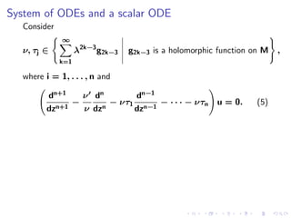
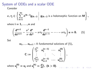
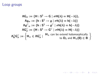
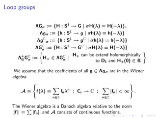
The document discusses harmonic maps from the Riemann surface M=S1×R or CP1\{0,1,∞} into the complex projective space CPn. It presents the DPW method for constructing harmonic maps using loop groups. Specifically, it constructs equivariant harmonic maps in CPn from degree one potentials in the loop algebra Λgσ, relating these to whether the maps are isotropic, weakly conformal, or non-conformal. It then considers the system of ODEs and scalar ODE that must be solved to generate the harmonic maps using this method.

1. Harmonic trinoids in complex projective spaces
Shimpei Kobayashi, Hirosaki University
12/12, 2008

2. Introduction
Harmonic maps into complex projective spaces
Preliminaries
Harmonic spheres
Harmonic tori
Equivariant harmonic maps in CPn
Isomorphisms between loop algebras
Potentials for equivariant harmonic maps
Harmonic trinoids in CPn
DPW method
System of ODEs and a scalar ODE
Hypergeometric equations
Unitarizability and interlace on the unit circle
Open problems

3. Let (M, g) and (N, h) be Riemannian manifolds and
Ψ : (M, g) → (N, h)
a C∞ map.
Define
E(Ψ) = |dΨ|2 dVg ,
M
where the norm is defined by g and h, and dV g is the volume form
of M.

4. Let (M, g) and (N, h) be Riemannian manifolds and
Ψ : (M, g) → (N, h)
a C∞ map.
Define
E(Ψ) = |dΨ|2 dVg ,
M
where the norm is defined by g and h, and dV g is the volume form
of M.
Consider the variation Ψt for Ψ.
def d
Ψ is harmonic ⇔ E(Ψt )|t=0 = 0 ⇔ τ (Ψ) = 0,
dt
where τ (Ψ) = trace dΨ is the tension field.

5. In particular, if dim M = 2, then the harmonicity can be written
as
Ψ ∂
∂ dΨ( ) = 0, (1)
∂¯
z ∂z
where z = x + iy and (x, y) is a conformal coordinate.

6. Harmonic spheres
If M = S2 , the followings (N, h) were studied in details:
Sn (RPn ) (Calabi, Chern)
CPn (D. Burns, Eells-Wood, Din-Zakrzewski, Glaser-Stora)
Gr2 (Cn ) (Chern-Wolfson, Burstall-Wood)
Grk (Cn ) (Wolfson, Wood)
These are based on
1) Holomorphic differential on S2 is zero
2) Techniques of Hermitian vector bundles.

7. Harmonic tori
If M = T2 , the followings (N, h) were studied in details :
S2 (Pinkall-Sterling)
S3 (Hitchin)
S4 (Pinkall-Ferus-Sterling-Pedit)
Sn , CPn (Burstall, McIntosh)
Gr2 (C4 ), HP3 (Udagawa)
Rank 1 compact symmetric spaces
(Burstall-Ferus-Pedit-Pinkall)
These are based on integrable system methods.

8. Goal of this talk
I would like to discuss harmonic maps from M = S 1 × R or
M = CP1 {0, 1, ∞} into N = CPn .

9. Goal of this talk
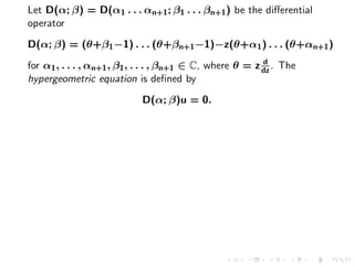
I would like to discuss harmonic maps from M = S 1 × R or
M = CP1 {0, 1, ∞} into N = CPn .
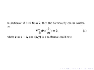
Consider a C∞ map Ψ from a Riemann surface M into a
symmetric space G/K:
∂ 1
Ψ dαk + 2 [αk ∧ αk ] = −[αp ∧ αp ] = 0,
∂ dΨ( )=0 ⇔
∂¯
z ∂z dαp + [αk ∧ αp ] = 0,
1
dαλ + 2 [αλ ∧ αλ ] = 0,
⇔
αλ = λ−1 αp + αk + λαp , λ ∈ S1 .
where α = F−1 dF is the Maurer-Cartan form of a lift
F : M → G, g = k ⊕ p and TMC = T M + T M.

10. Equivariant harmonic maps in k-symmetric spaces
Definition
A map Ψ : R2 → G/K is called R-equivariant if
Ψ(x, y) = exp(xA0 )Φ(y),
for some A0 ∈ g and Φ : R → G/K.
Theorem (Burstall-Kilian)
All equivariant primitive harmonic maps in k-symmetric spaces
G/K (with an order k-automorphism τ ) are constructed from
degree one potentials:
ξ = λ−1 ξ−1 + ξ0 + λξ1 ∈ Λgτ , (2)
where Λgτ = {ξ : S1 → g | ξ(e2πi/k λ) = τ ξ(λ)} is the loop
algebra of the Lie algebra g of G, ξj ∈ gj and ξj = ξ−j with the
eigenspace decomposition of gC = i∈Zk gi .

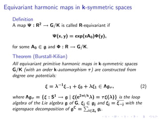
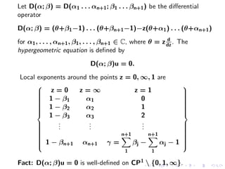
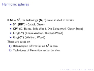
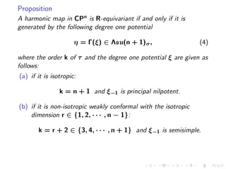
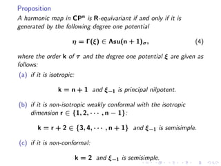
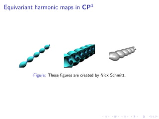
11. Equivariant harmonic maps in CPn
For CPn case, G = SU(n + 1) with the involution
σ = Ad diag [1, −1, . . . , −1], thus K = S(U(1) × U(n)) and
GC = SL(n + 1, C).
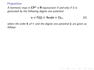
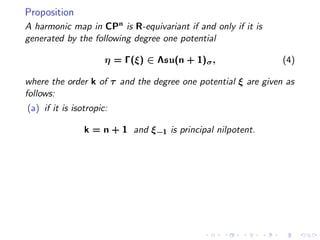
It is known that harmonic maps in CPn can be classified into
isotropic,
non-isotropic weakly conformal with isotropic dimension
r ∈ {1, . . . , n − 1},
non-conformal.
Problem: Which degree one potentials are corresponding to the
above cases?

12. Isomorphism
Lemma (Pacheco)
Let g be a Lie algebra, τ : g → g an automorphism of order k
and σ : g → g an involution.
Define Γ as a map between Λgτ and Λgσ
Γ(ξ)(λ) = s(λ)t(λ−2/k )ξ(λ2/k ) ∈ Λgσ for ξ ∈ Λgτ , (3)
where t : S1 → Aut g and s : S1 → Aut g are automorphism
such that t(e2πi/k ) = τ and s(−1) = σ respectively.
Then Γ is an isomorphism.

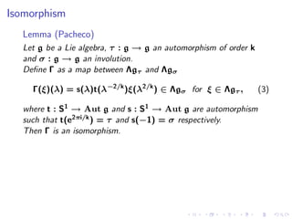
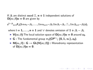
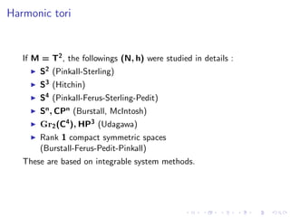
13. Isomorphism
Lemma (Pacheco)
Let g be a Lie algebra, τ : g → g an automorphism of order k
and σ : g → g an involution.
Define Γ as a map between Λgτ and Λgσ
Γ(ξ)(λ) = s(λ)t(λ−2/k )ξ(λ2/k ) ∈ Λgσ for ξ ∈ Λgτ , (3)
where t : S1 → Aut g and s : S1 → Aut g are automorphism
such that t(e2πi/k ) = τ and s(−1) = σ respectively.
Then Γ is an isomorphism.
Let t and s be t(λ) = Ad diag[1, λ, . . . , λ k−2 , λk−1 , . . . , λk−1 ]
and s(λ) = Ad diag[1, λ, . . . , λ] respectively. Then it is easy to
see t(e2πi/k ) = τ and s(−1) = σ. Define Γ as in (3), and let
t
ξ = λ−1 ξ−1 + ξ0 + λξ−1 ∈ Λsu(n + 1)τ
be the degree one potential.

14. Proposition
A harmonic map in CPn is R-equivariant if and only if it is
generated by the following degree one potential
η = Γ(ξ) ∈ Λsu(n + 1)σ , (4)
where the order k of τ and the degree one potential ξ are given as
follows:

15. Proposition
A harmonic map in CPn is R-equivariant if and only if it is
generated by the following degree one potential
η = Γ(ξ) ∈ Λsu(n + 1)σ , (4)
where the order k of τ and the degree one potential ξ are given as
follows:
(a) if it is isotropic:
k = n + 1 and ξ−1 is principal nilpotent.

16. Proposition
A harmonic map in CPn is R-equivariant if and only if it is
generated by the following degree one potential
η = Γ(ξ) ∈ Λsu(n + 1)σ , (4)
where the order k of τ and the degree one potential ξ are given as
follows:
(a) if it is isotropic:
k = n + 1 and ξ−1 is principal nilpotent.
(b) if it is non-isotropic weakly conformal with the isotropic
dimension r ∈ {1, 2, · · · , n − 1}:
k = r + 2 ∈ {3, 4, · · · , n + 1} and ξ−1 is semisimple.

17. Proposition
A harmonic map in CPn is R-equivariant if and only if it is
generated by the following degree one potential
η = Γ(ξ) ∈ Λsu(n + 1)σ , (4)
where the order k of τ and the degree one potential ξ are given as
follows:
(a) if it is isotropic:
k = n + 1 and ξ−1 is principal nilpotent.
(b) if it is non-isotropic weakly conformal with the isotropic
dimension r ∈ {1, 2, · · · , n − 1}:
k = r + 2 ∈ {3, 4, · · · , n + 1} and ξ−1 is semisimple.
(c) if it is non-conformal:
k = 2 and ξ−1 is semisimple.

18. Equivariant harmonic maps in CP1
Figure: These figures are created by Nick Schmitt.

19. Loop groups
Definition
G : A compact simple Lie group, g : Lie algebra of G,
GC : The complexification of G, gC : Lie algebra of GC ,
σ : A involution of G, K : The fixed point set of σ
k : Lie algebra of K, g = k ⊕ p : Direct sum
B : The solvable part of an Iwasawa decomposition
KC = K · B, K ∩ B = e

20. Loop groups
ΛGσ := {H : S1 → G | σH(λ) = H(−λ)},
Λgσ := {h : S1 → g | σh(λ) = h(−λ)}
ΛgC σ := {h : S1 → gC | σh(λ) = h(−λ)}
ΛGC := {H : S1 → GC | σH(λ) = H(−λ)}
σ
H+ can be extend holomorphically
Λ+ GC :=
B σ H+ ∈ ΛGC |
σ to D1 and H+ (0) ∈ B

21. Loop groups
ΛGσ := {H : S1 → G | σH(λ) = H(−λ)},
Λgσ := {h : S1 → g | σh(λ) = h(−λ)}
ΛgC σ := {h : S1 → gC | σh(λ) = h(−λ)}
ΛGC := {H : S1 → GC | σH(λ) = H(−λ)}
σ
H+ can be extend holomorphically
Λ+ GC :=
B σ H+ ∈ ΛGC |
σ to D1 and H+ (0) ∈ B
We assume that the coefficients of all g ∈ Λg σ are in the Wiener
algebra
A= f(λ) = fn λn : C r → C ; |fn | < ∞ .
n∈Z n∈Z
The Wiener algebra is a Banach algebra relative to the norm
f = |fn |, and A consists of continuous functions.

22. DPW method
Step1 η(z, λ) = ∞ λk ξk (z) : ΛgC -valued 1-form on Σ ⊂ C,
k=−1 σ
where ξeven (z) ∈ Ω1,0 (kC ) and ξodd (z) ∈ Ω1,0 (pC ).
Step2 Solve ODE dC = Cη.
Step3 Iwasawa decomposition : C = FW + , F : Σ → ΛGσ and
W+ : Σ → Λ + GC .
B σ
Step4 Projection π ◦ F|λ∈S1 : Σ → G/K, where π : G → G/K.
Theorem (Dorfmeister-Pedit-Wu)
Multiplication ΛGσ × Λ+ GC → ΛGC is a diffeomorphism onto.
B σ σ
Theorem (Dorfmeister-Pedit-Wu, 1998)
Every harmonic map from a simply connected domain Σ into G/K
can be constructed in this way.

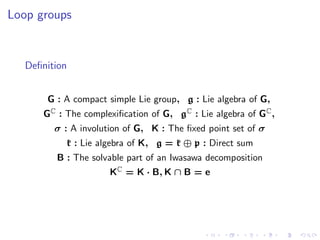
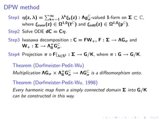
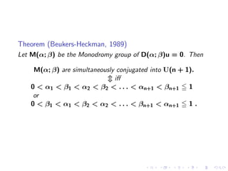
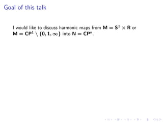
23. DPW method
Step1 η(z, λ) = ∞ λk ξk (z) : ΛgC -valued 1-form on Σ ⊂ C,
k=−1 σ
where ξeven (z) ∈ Ω1,0 (kC ) and ξodd (z) ∈ Ω1,0 (pC ).
Step2 Solve ODE dC = Cη.
Step3 Iwasawa decomposition : C = FW + , F : Σ → ΛGσ and
W+ : Σ → Λ + GC .
B σ
Step4 Projection π ◦ F|λ∈S1 : Σ → G/K, where π : G → G/K.
Theorem (Dorfmeister-Pedit-Wu)
Multiplication ΛGσ × Λ+ GC → ΛGC is a diffeomorphism onto.
B σ σ
Theorem (Dorfmeister-Pedit-Wu, 1998)
Every harmonic map from a simply connected domain Σ into G/K
can be constructed in this way.
From now on, CPn is represented as the symmetric space
U(n + 1)/U(1) × U(n) with the involution
σ = Ad diag [1, −1, . . . , −1].

24. System of ODEs and a scalar ODE
Consider
∞
ν, τj ∈ λ2k−3 g2k−3 g2k−3 is a holomorphic function on M ,
k=1
where i = 1, . . . , n and
dn+1 ν dn dn−1
− − ντ1 n−1 − · · · − ντn u = 0. (5)
dzn+1 ν dzn dz

25. System of ODEs and a scalar ODE
Consider
∞
ν, τj ∈ λ2k−3 g2k−3 g2k−3 is a holomorphic function on M ,
k=1
where i = 1, . . . , n and
dn+1 ν dn dn−1
− − ντ1 n−1 − · · · − ντn u = 0. (5)
dzn+1 ν dzn dz
Set
u1 , . . . un+1 : A fundamental solutions of (5),
 (n) 
u1 (n−1) (0)
 ν u1 · · · u1 
 . . .
. .. . 
.
C :=  . . . . ,
 (n) 
un+1 (n−1) (0)
ν
un+1 · · · un+1
(0) (k) dk u
where uj = uj and uj = dzk
, (k > 0).

26. Lemma
(1)  
0 ν 0 ··· 0

 τ1 0 1 · · · 0 

−1
 . . ..
. . .. .
. 
η := C dC =  . . . . . . (6)
. . ..
 
 . . .. 
 . . . . 1 
τn 0 · · · · · · 0
∞
(2) η = λk ξk is a holomorphic potential on M, where
k −1
ξeven ∈ Ω1,0 (kC ) and ξodd ∈ Ω1,0 (pC ).
Fact: Monodromy representations of (5) and (6) are the same.

27. Hypergeometric functions
n+1 Fn (α1 , . . . , αn+1 ; β1 , . . . , βn |z)
∞
(α1 )k · · · (αn+1 )k k
= z , (7)
k=0
(β1 )k · · · (βn )k k!
where α1 , . . . , αn+1 , β1 , . . . , βn ∈ C, (x)k is the Pochhammer
symbol or rising factorial
Γ(x + k)
(x)k = = x(x + 1) · · · (x + k − 1).
Γ(x)
n+1 Fn (α1 , . . . , αn+1 ; β1 , . . . , βn |z) is called the
hypergeometric function n+1 Fn .
2 F1 (α1 , α2 ; β1 |z) is the Gauß’s hypergeometric function.

28. Let D(α; β) = D(α1 . . . αn+1 ; β1 . . . βn+1 ) be the differential
operator
D(α; β) = (θ+β1 −1) . . . (θ+βn+1 −1)−z(θ+α1 ) . . . (θ+αn+1 )
d
for α1 , . . . , αn+1 , β1 , . . . , βn+1 ∈ C, where θ = z dz . The
hypergeometric equation is defined by
D(α; β)u = 0.

29. Let D(α; β) = D(α1 . . . αn+1 ; β1 . . . βn+1 ) be the differential
operator
D(α; β) = (θ+β1 −1) . . . (θ+βn+1 −1)−z(θ+α1 ) . . . (θ+αn+1 )
d
for α1 , . . . , αn+1 , β1 , . . . , βn+1 ∈ C, where θ = z dz . The
hypergeometric equation is defined by
D(α; β)u = 0.
Local exponents around the points z = 0, ∞, 1 are
 
 z=0
 z=∞ z=1 

 1−β α1 0 


 1 


 1 − β2

 α2 1



 
1 − β3 α3 2
 
.
. .
. .
.



 . . . 





 n+1 n+1 


 1 − βn+1 αn+1 γ =

 βj − αj − 1



 
1 1
Fact: D(α; β)u = 0 is well-defined on CP 1 {0, 1, ∞}.

30. If βi are distinct mod Z, n + 1 independent solutions of
D(α; β)u = 0 are given by
z1−βi n+1 Fn (1+α1 −βi , . . . , 1+αn+1 −βi ; 1+β1 −βi , . ∨ ., 1+βn+1 −βi |z),
.
where i = 1, . . . , n + 1 and ∨ denotes omission of 1 + β i − βi .
V(α; β):The local solution space of D(α; β)u = 0 around z 0 .
G : The fundamental group π1 (CP1 {0, 1, ∞}, z0 ).
M(α, β) : G → GL(V(α; β)) : Monodromy representation
of D(α; β)u = 0.

31. Theorem (Beukers-Heckman, 1989)
Let M(α; β) be the Monodromy group of D(α; β)u = 0. Then
M(α; β) are simultaneously conjugated into U(n + 1).
iff
0 < α1 < β1 < α2 < β2 < . . . < αn+1 < βn+1 1
or
0 < β1 < α1 < β2 < α2 < . . . < βn+1 < αn+1 1 .

32. Remark
αj and βj are determined by solving the indicial equations, which
are n-th order algebraic equations.
There are several problems for an application to harmonic maps in
CPn .
αj and βj depend on the additional parameter λ ∈ C.
αj and βj need to be real and satisfy the inequality for almost
all λ ∈ S1 .
Products and sums of αj and βj are ν and τj as in the
holomorphic potential of (6).

33. The case n = 1 (Gauß’s hypergeometric equation)
Local exponents
 
 z=0
 z=∞ z=1 

 1−β α1 0 
 1 
2 2
 1 − β2

 α2 γ= βj − αj − 1 


 
1 1
Set
α1 = 1 − v 1 − v 2 − v 3 , α 2 = 1 − v 1 − v 2 + v 3 ,
and
β1 = 1 − 2v1 , β2 = 1,
where
1 1
vj = − 1 + wj (λ − λ−1 )2
2 2

34. Spherical triangle inequality

 v1 + v 2 + v 3 < 1

v1 < v 2 + v 3

0 < α 1 < β1 < α2 < β2 1⇔ (8)
 v2 < v 1 + v 3

v3 < v 1 + v 2

It is not difficult to show that the above inequality are satisfied for
some choices of wj . Moreover all problems can be solved
(Kilian-Kobayashi-Rossman-Schmitt, Dorfmeister-Wu).
Remark
Umehara-Yamada considered the similar inequality for CMC
H=1 in H3 . (No λ dependence!)

35. Examples of CMC trinoids in space forms
Figure: These figures are created by Nick Schmitt.

36. The case n > 1
Example
For the isotropic case, αj and βj do not depend on λ. Thus
there exist isotropic harmonic trinoids in CP n .
For n = 2, 3, the indicial equation can be solved explicitly.
We can show that there exist examples of harmonic trinoids in
CP2 and CP3 .

37. Open problem
What are behaviors around the punctures? Are they
asymptotically converge to equivariant ones?
Prove the existence of non-isotropic harmonic trinoids for
n 4.