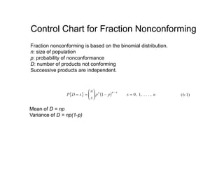
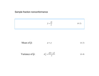
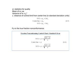
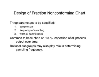
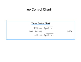
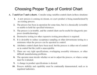
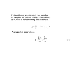
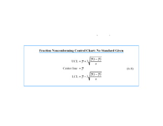
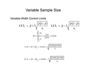
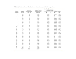
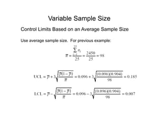
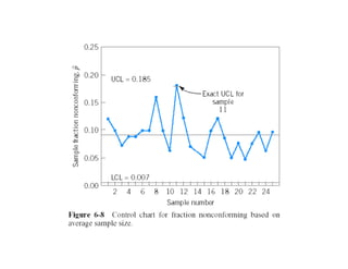
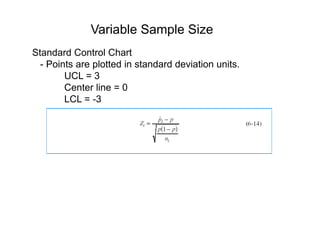
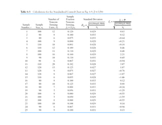
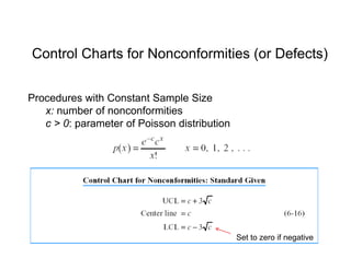
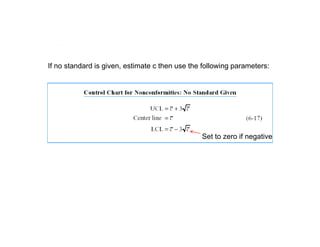
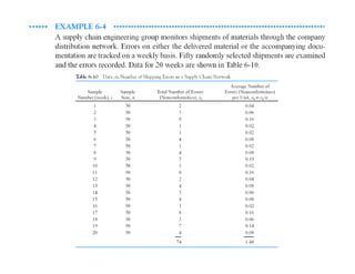
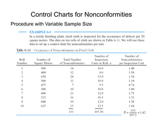
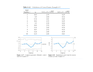
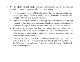
This document discusses control charts for attributes, including fraction nonconforming charts and control charts for nonconformities (defects). It covers key aspects such as: 1. The parameters, formulas, and design of fraction nonconforming charts, including sample size, frequency of sampling, and control limit width. 2. Procedures for control charts with constant and variable sample sizes, and how to estimate parameters if a standard is not given. 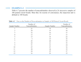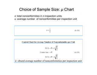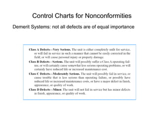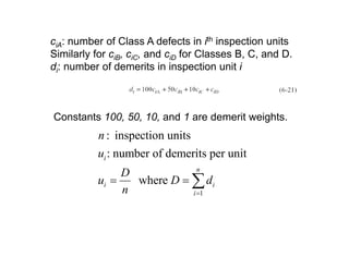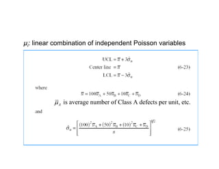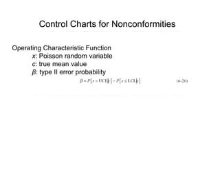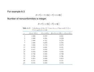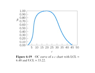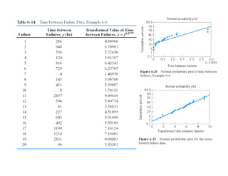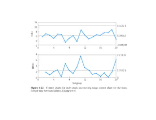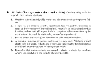3. How to construct control charts to monitor nonconformities using variables like number of defects, demerit points, and Poisson distributions. 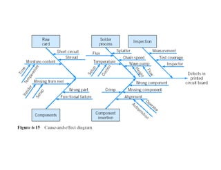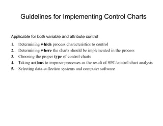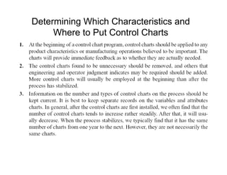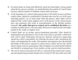4. Guidelines for implementing control charts and determining which characteristics and processes to monitor.

1. Chapter 7. Control Charts for Attributes

2. Control Chart for Fraction Nonconformingg
Fraction nonconforming is based on the binomial distribution.
n: size of populationp p
p: probability of nonconformance
D: number of products not conforming
Successive products are independent.
Mean of D = np
Variance of D = np(1-p)

3. Sample fraction nonconformance
ˆMean of p:Mean of p:
ˆVariance of p:

4. w: statistics for quality
Mean of w: µwMean of w: µw
Variance of w: σw
2
L: distance of control limit from center line (in standard deviation units)
If p is the true fraction nonconformance:

5. If p is not know, we estimate it from samples.
m: samples, each with n units (or observations)
D: number of nonconforming units in sample iDi: number of nonconforming units in sample i
Average of all observations:

7. Example 6-1. 6-oz cardboard cans of orange juice

8. Design of Fraction Nonconforming ChartDesign of Fraction Nonconforming Chart
Three parameters to be specified:p p
1. sample size
2. frequency of sampling
3 width of control limits3. width of control limits
Common to base chart on 100% inspection of all process
output over time.
Rational subgroups may also play role in determining
sampling frequency.

9. np Control Chart

10. Variable Sample Size
Variable-Width Control Limits
( ) ( )( ) ( )1- 1-
UCL 3 LCL 3
i i
p p p p
p p
n n
= + = −

12. Variable Sample Size
Control Limits Based on an Average Sample Size
U l i F i lUse average sample size. For previous example:

14. Variable Sample Size
Standard Control Chart
- Points are plotted in standard deviation units.
UCL = 3UCL = 3
Center line = 0
LCL = -3

16. Operating Characteristic Function andOperating Characteristic Function and
Average Run Length Calculations
Probability of type II error
{ } { }
{ } { }
ˆ ˆUCL | LCL |
UCL | LCL |
P p p P p p
P D n p P D n p
β = < − ≤
< ≤{ } { }UCL | LCL |P D n p P D n p= < − ≤

17. C t l Ch t f N f iti ( D f t )Control Charts for Nonconformities (or Defects)
Procedures with Constant Sample Size
x: number of nonconformities
c > 0: parameter of Poisson distribution
Set to zero if negative

18. If no standard is given, estimate c then use the following parameters:
Set to zero if negativeg

21. Choice of Sample Size: µ Chart
x: total nonconformities in n inspection units
u: average number of nonconformities per inspection unit
: obserd average number of nonconformities per inspection unitu: obserd average number of nonconformities per inspection unitu

23. Control Charts for Nonconformities
Procedure with Variable Sample SizeProcedure with Variable Sample Size

25. Control Charts for Nonconformities
Demerit Systems: not all defects are of equal importance

26. ciA: number of Class A defects in ith inspection units
Similarly for ciB, ciC, and ciD for Classes B, C, and D.
di: number of demerits in inspection unit i
Constants 100 50 10 and 1 are demerit weightsConstants 100, 50, 10, and 1 are demerit weights.
: inspection units
b f d it it
n
: number of demerits per unit
where
i
n
i i
u
D
u D d= = ∑1
i i
in =
∑

27. µi: linear combination of independent Poisson variables
is average number of Class A defects per unit, etc.Aµ

28. Control Charts for Nonconformities
Operating Characteristic Function
x: Poisson random variable
c: true mean value
β: type II error probabilityβ ype e o p obab y

29. For example 6-3
Number of nonconformities is integer.

31. Control Charts for Nonconformities
• If defect level is low, <1000 per million, c and u charts become
ineffective
Dealing with Low Defect Levels
ineffective.
• The time-between-events control chart is more effective.
• If the defects occur according to a Poisson distribution, the
probability distribution of the time between events is the exponentialp y p
distribution.
• Constructing a time-between-events control chart is essentially
equivalent to control charting an exponentially distributed variable.
• To use normal approximation translate exponential distribution to• To use normal approximation, translate exponential distribution to
Weibull distribution and then approximate with normal variable
: normal approximation for exponential variablex y
1
0.27773.6
x y y= =

35. Guidelines for Implementing Control Charts
Applicable for both variable and attribute control

36. Determining Which Characteristics and
Where to Put Control ChartsWhere to Put Control Charts

38. Choosing Proper Type of Control Chart

41. Actions Taken to Improve Process