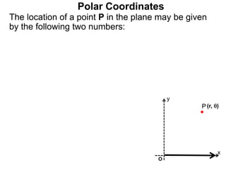
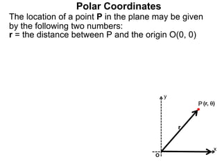
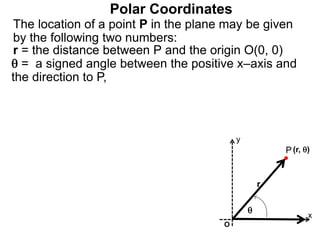
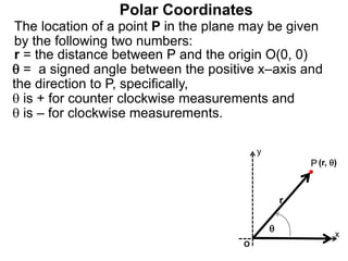
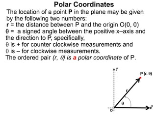
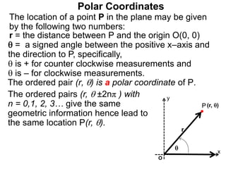
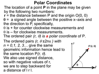
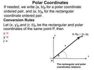
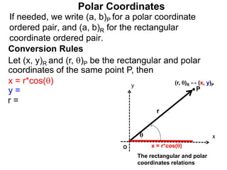
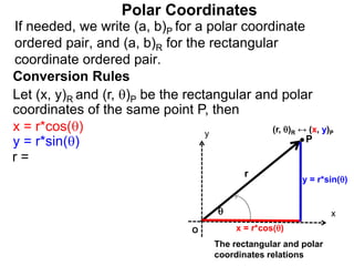
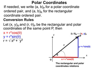
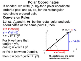
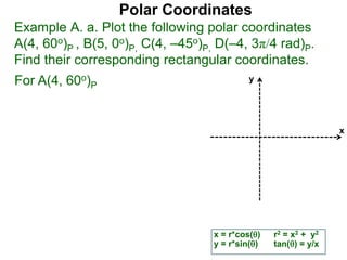
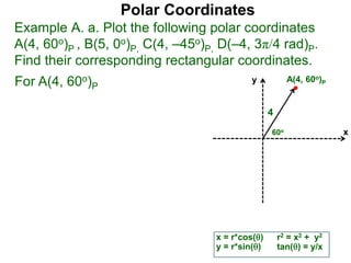
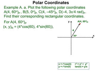
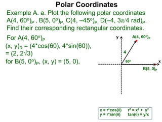
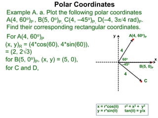
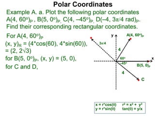
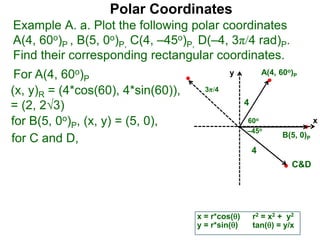
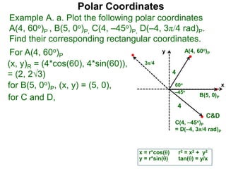
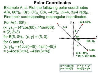
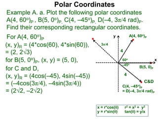
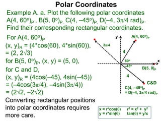
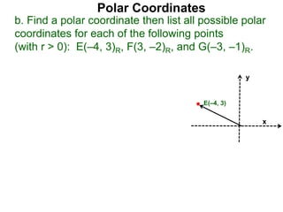
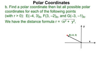
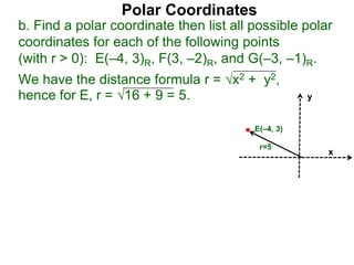
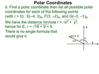
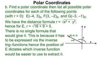
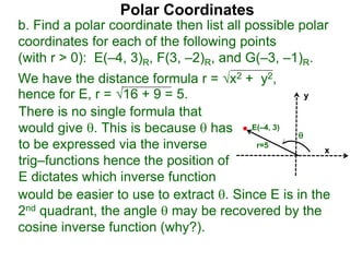
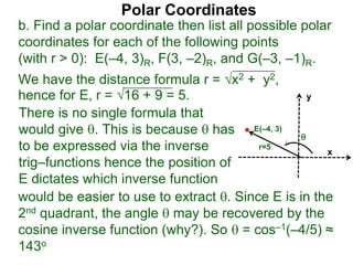
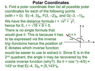
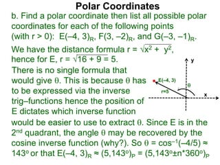
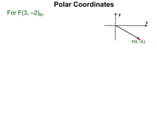
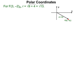
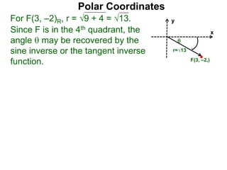
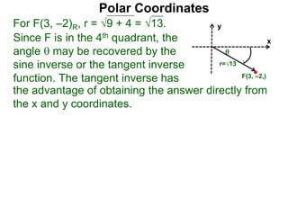
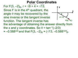
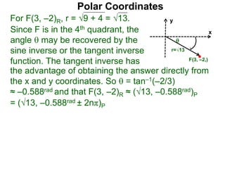
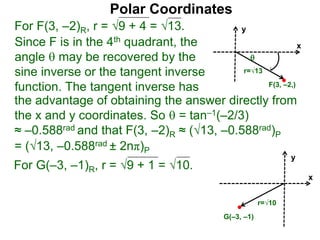
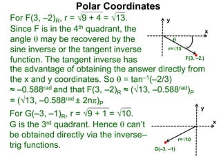
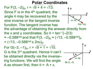
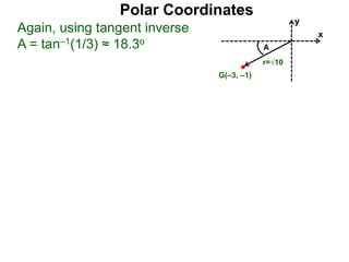
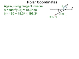
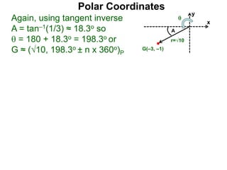
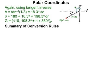
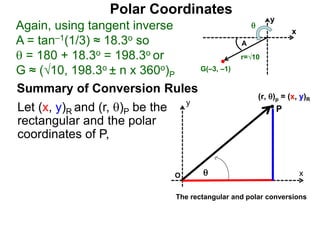
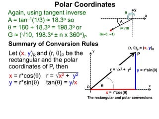
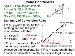
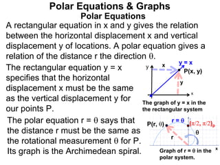
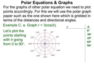
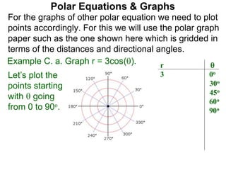
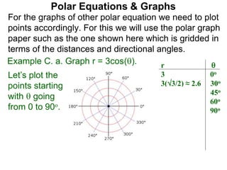
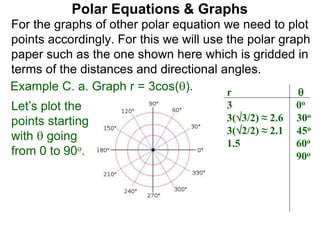
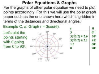
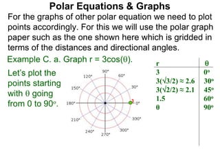
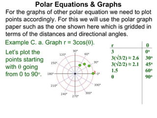
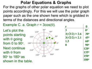
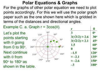
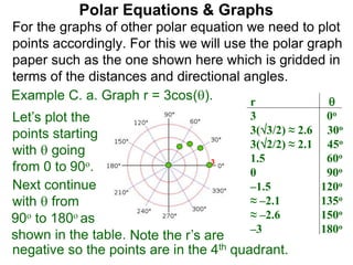
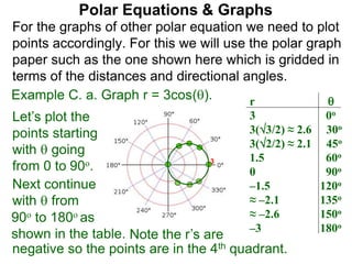
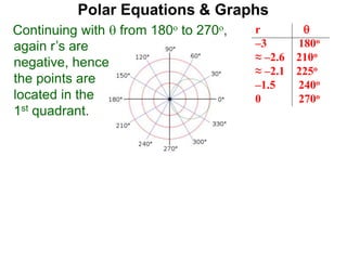
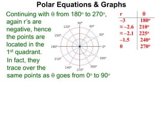
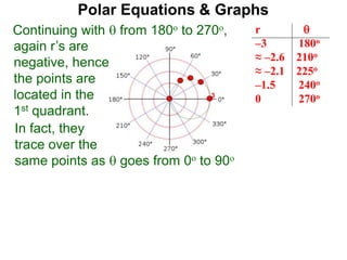
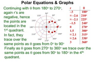
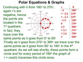
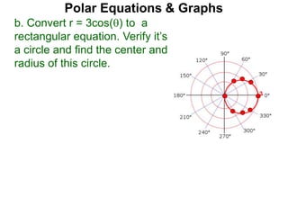
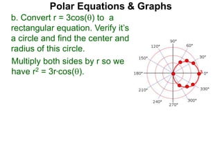
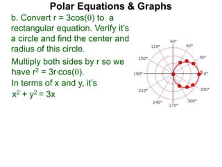
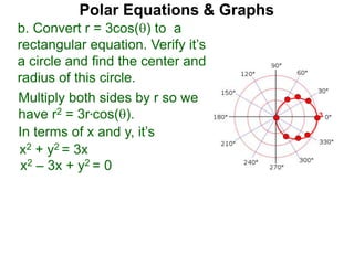
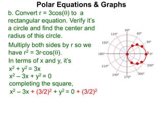
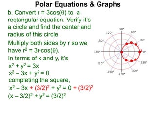
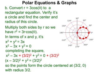
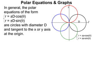
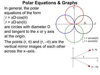
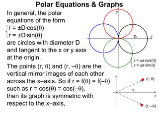
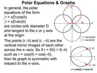
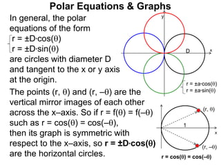
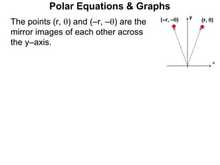
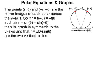
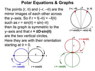
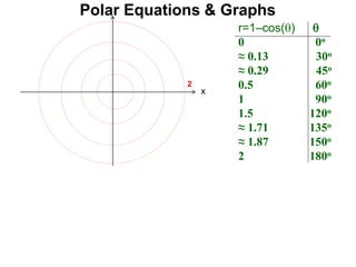
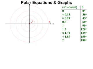
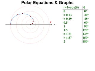
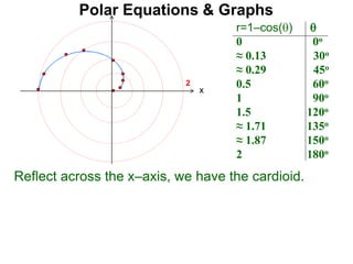
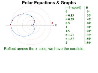
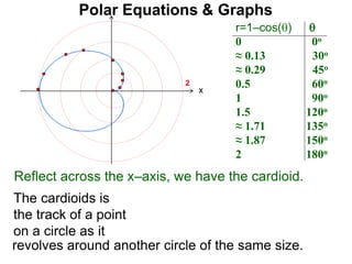
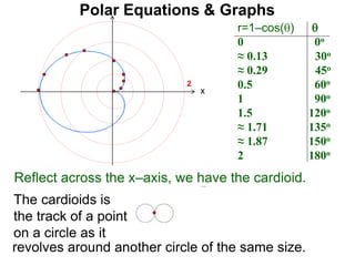
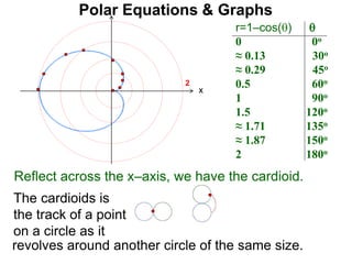
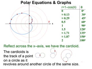
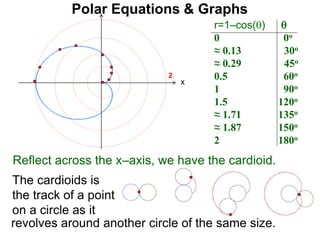
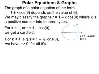
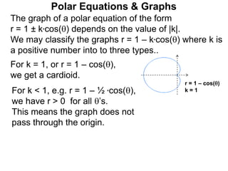
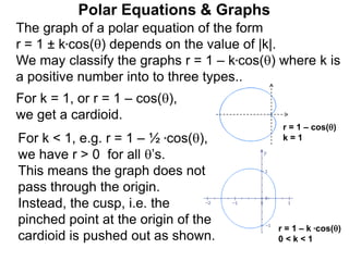
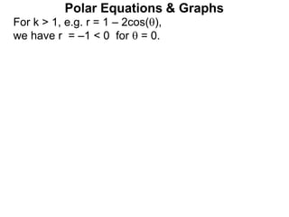
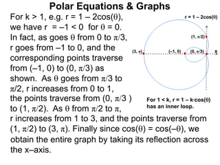
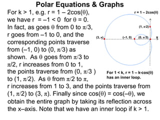
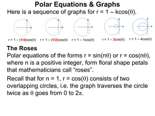
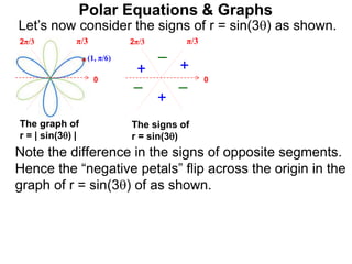
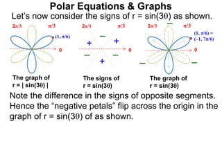
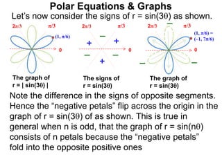
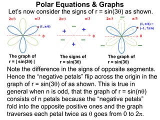
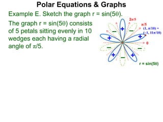
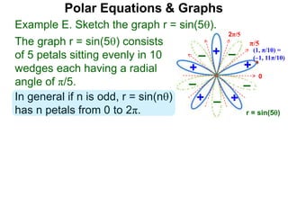
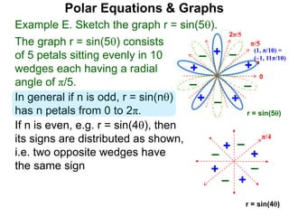
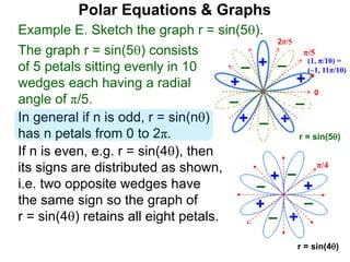
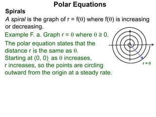
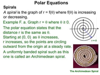
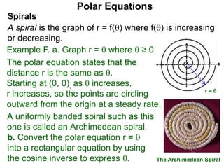
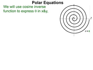
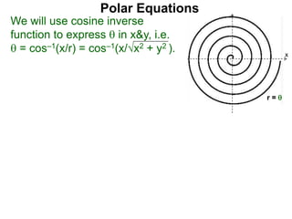
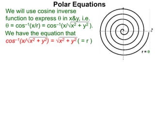
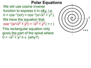
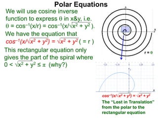
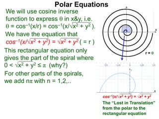
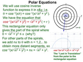
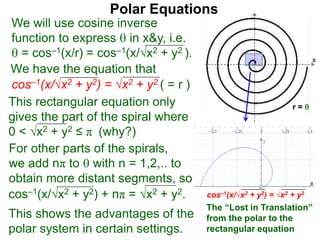
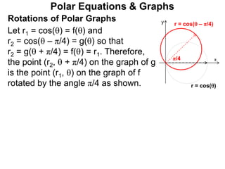
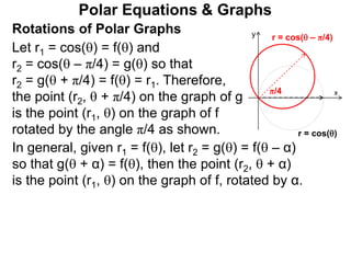
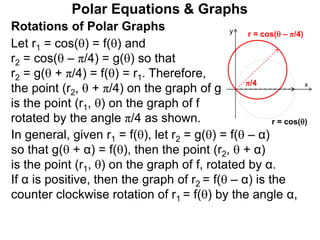
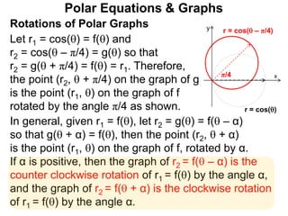
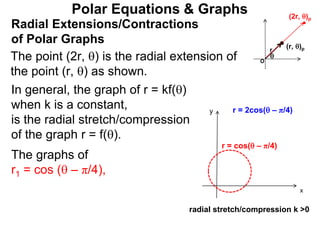
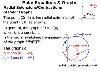
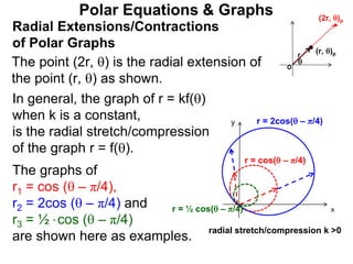
34 polar coordinate and equations

Polar Coordinates
The location of a point P in the plane may be given
by the following two numbers:
P
x
y
(r, )
O

Polar Coordinates
r = the distance between P and the origin O(0, 0)
P
x
(r, )
r
O
y

Polar Coordinates
 = a signed angle between the positive x–axis and
the direction to P,
P
x
(r, )

r
O
y

Polar Coordinates
the direction to P, specifically,
 is + for counter clockwise measurements and
 is – for clockwise measurements.
P
x
(r, )

r
O
y

Polar Coordinates
The ordered pair (r, ) is a polar coordinate of P.
P
x
(r, )

r
O
y

Polar Coordinates
P
x
(r, )

r
The ordered pairs (r,  ±2nπ ) with
n = 0,1, 2, 3… give the same
geometric information hence lead to
the same location P(r, ).
O
y

Polar Coordinates
P
x
(r, )

r
The ordered pairs (r,  ±2nπ ) with
n = 0,1, 2, 3… give the same
geometric information hence lead to
the same location P(r, ).
We also use signed distance,
so with negative values of r,
we are to step backward for
a distance of l r l. O
y

Polar Coordinates
If needed, we write (a, b)P for a polar coordinate
ordered pair, and (a, b)R for the rectangular
coordinate ordered pair.

Polar Coordinates
Conversion Rules

Polar Coordinates
Conversion Rules
Let (x, y)R and (r, )P be the rectangular and polar
coordinates of the same point P, then
P
x
y

r
O
The rectangular and polar
coordinates relations
x =
y =
r =
(r, )R ↔ (x, y)P

Polar Coordinates
Conversion Rules
P
x
y (r, )R ↔ (x, y)P

r
O x = r*cos()
x = r*cos()
y =
r =

Polar Coordinates
Conversion Rules
P
x
y

r
O x = r*cos()
x = r*cos()
y = r*sin()
y = r*sin()
r =
(r, )R ↔ (x, y)P

Polar Coordinates
Conversion Rules
P
x
y

r
O x = r*cos()
y = r*sin()
x = r*cos()
y = r*sin()
r = √ x2 + y2
(r, )R ↔ (x, y)P

Polar Coordinates
Conversion Rules
P
x
y

r
O x = r*cos()
y = r*sin()
x = r*cos()
y = r*sin()
r = √ x2 + y2
For  we have that
tan() = y/x,
cos() = x/√x2 + y2
or if  is between 0 and π,
then  = cos–1 (x/√x2 + y2).
(r, )R ↔ (x, y)P

Polar Coordinates
Example A. a. Plot the following polar coordinates
A(4, 60o)P , B(5, 0o)P, C(4, –45o)P, D(–4, 3π/4 rad)P.
Find their corresponding rectangular coordinates.

Polar Coordinates
x
y
x = r*cos()
y = r*sin()
r2 = x2 + y2
tan() = y/x
For A(4, 60o)P

Polar Coordinates
x
y
60o
4
x = r*cos()
y = r*sin()
A(4, 60o)P
r2 = x2 + y2
tan() = y/x
For A(4, 60o)P

Polar Coordinates
For A(4, 60o)P
x = r*cos()
y = r*sin()
(x, y)R = (4*cos(60), 4*sin(60)),
r2 = x2 + y2
tan() = y/x
x
y
60o
4
A(4, 60o)P

Polar Coordinates
For A(4, 60o)P
x = r*cos()
y = r*sin()
(x, y)R = (4*cos(60), 4*sin(60)),
= (2, 23)
r2 = x2 + y2
tan() = y/x
x
y
60o
4
A(4, 60o)P

Polar Coordinates
For A(4, 60o)P
x = r*cos()
y = r*sin()
(x, y)R = (4*cos(60), 4*sin(60)),
= (2, 23)
for B(5, 0o)P, (x, y) = (5, 0),
r2 = x2 + y2
tan() = y/x
x
y
60o
4
A(4, 60o)P
B(5, 0)P

Polar Coordinates
x
y
60o
4
For A(4, 60o)P
x = r*cos()
y = r*sin()
(x, y)R = (4*cos(60), 4*sin(60)),
= (2, 23)
for B(5, 0o)P, (x, y) = (5, 0),
for C and D,
A(4, 60o)P
B(5, 0)P
4
r2 = x2 + y2
tan() = y/x
–45o
C

Polar Coordinates
x
y
60o
4
For A(4, 60o)P
x = r*cos()
y = r*sin()
(x, y)R = (4*cos(60), 4*sin(60)),
= (2, 23)
for B(5, 0o)P, (x, y) = (5, 0),
for C and D,
A(4, 60o)P
B(5, 0)P
4
r2 = x2 + y2
tan() = y/x
–45o
3π/4
C

Polar Coordinates
x
y
60o
4
For A(4, 60o)P
x = r*cos()
y = r*sin()
(x, y)R = (4*cos(60), 4*sin(60)),
= (2, 23)
for B(5, 0o)P, (x, y) = (5, 0),
for C and D,
A(4, 60o)P
B(5, 0)P
4
r2 = x2 + y2
tan() = y/x
–45o
3π/4
C&D

Polar Coordinates
x
y
60o
4
For A(4, 60o)P
x = r*cos()
y = r*sin()
(x, y)R = (4*cos(60), 4*sin(60)),
= (2, 23)
for B(5, 0o)P, (x, y) = (5, 0),
for C and D,
A(4, 60o)P
B(5, 0)P
C(4, –45o)P
= D(–4, 3π/4 rad)P
4
r2 = x2 + y2
tan() = y/x
–45o
3π/4
C&D

Polar Coordinates
x
y
60o
4
For A(4, 60o)P
x = r*cos()
y = r*sin()
(x, y)R = (4*cos(60), 4*sin(60)),
= (2, 23)
for B(5, 0o)P, (x, y) = (5, 0),
for C and D,
(x, y)R = (4cos(–45), 4sin(–45))
= (–4cos(3π/4), –4sin(3π/4))
A(4, 60o)P
B(5, 0)P
C(4, –45o)P
= D(–4, 3π/4 rad)P
4
r2 = x2 + y2
tan() = y/x
–45o
3π/4
C&D

Polar Coordinates
x
y
60o
4
For A(4, 60o)P
x = r*cos()
y = r*sin()
(x, y)R = (4*cos(60), 4*sin(60)),
= (2, 23)
for B(5, 0o)P, (x, y) = (5, 0),
for C and D,
(x, y)R = (4cos(–45), 4sin(–45))
= (–4cos(3π/4), –4sin(3π/4))
= (22, –22)
A(4, 60o)P
B(5, 0)P
C(4, –45o)P
= D(–4, 3π/4 rad)P
4
r2 = x2 + y2
tan() = y/x
–45o
3π/4
C&D

Polar Coordinates
x
y
60o
4
For A(4, 60o)P
x = r*cos()
y = r*sin()
(x, y)R = (4*cos(60), 4*sin(60)),
= (2, 23)
for B(5, 0o)P, (x, y) = (5, 0),
for C and D,
(x, y)R = (4cos(–45), 4sin(–45))
= (–4cos(3π/4), –4sin(3π/4))
= (22, –22)
A(4, 60o)P
B(5, 0)P
C(4, –45o)P
= D(–4, 3π/4 rad)P
4
Converting rectangular positions
into polar coordinates requires
more care.
r2 = x2 + y2
tan() = y/x
–45o
3π/4
C&D

Polar Coordinates
b. Find a polar coordinate then list all possible polar
coordinates for each of the following points
(with r > 0): E(–4, 3)R, F(3, –2)R, and G(–3, –1)R.

Polar Coordinates
(with r > 0): E(–4, 3)R, F(3, –2)R, and G(–3, –1)R.
x
y
E(–4, 3)

Polar Coordinates
(with r > 0): E(–4, 3)R, F(3, –2)R, and G(–3, –1)R.
We have the distance formula r = x2 + y2,
x
y
E(–4, 3)

Polar Coordinates
(with r > 0): E(–4, 3)R, F(3, –2)R, and G(–3, –1)R.
hence for E, r = 16 + 9 = 5.
x
y
E(–4, 3)
r=5

Polar Coordinates
(with r > 0): E(–4, 3)R, F(3, –2)R, and G(–3, –1)R.
There is no single formula that
would give .
hence for E, r = 16 + 9 = 5.
x
y
E(–4, 3)
r=5


Polar Coordinates
(with r > 0): E(–4, 3)R, F(3, –2)R, and G(–3, –1)R.
would give . This is because  has
to be expressed via the inverse
trig–functions hence the position of
E dictates which inverse function
hence for E, r = 16 + 9 = 5.
would be easier to use to extract .
x
y
E(–4, 3)
r=5


Polar Coordinates
(with r > 0): E(–4, 3)R, F(3, –2)R, and G(–3, –1)R.
hence for E, r = 16 + 9 = 5.
would be easier to use to extract . Since E is in the
2nd quadrant, the angle  may be recovered by the
cosine inverse function (why?).
x
y
E(–4, 3)
r=5


Polar Coordinates
(with r > 0): E(–4, 3)R, F(3, –2)R, and G(–3, –1)R.
hence for E, r = 16 + 9 = 5.
x
y
E(–4, 3)

r=5
cosine inverse function (why?). So  = cos–1(–4/5) ≈
143o

Polar Coordinates
(with r > 0): E(–4, 3)R, F(3, –2)R, and G(–3, –1)R.
hence for E, r = 16 + 9 = 5.
x
y
E(–4, 3)

r=5
143o or that E(–4, 3)R ≈ (5,143o)P

Polar Coordinates
(with r > 0): E(–4, 3)R, F(3, –2)R, and G(–3, –1)R.
hence for E, r = 16 + 9 = 5.
x
y
E(–4, 3)

r=5
143o or that E(–4, 3)R ≈ (5,143o)P = (5,143o±n*360o)P

Polar Coordinates
For F(3, –2)R,
x
y
F(3, –2,)

Polar Coordinates
For F(3, –2)R, r = 9 + 4 = √13.
x
y
F(3, –2,)
r=√13

Polar Coordinates
For F(3, –2)R, r = 9 + 4 = √13.
x
y
F(3, –2,)
Since F is in the 4th quadrant, the
angle  may be recovered by the
sine inverse or the tangent inverse
function.

r=√13

Polar Coordinates
For F(3, –2)R, r = 9 + 4 = √13.
x
y
F(3, –2,)
function. The tangent inverse has
the advantage of obtaining the answer directly from
the x and y coordinates.

r=√13

Polar Coordinates
For F(3, –2)R, r = 9 + 4 = √13.
x
y
F(3, –2,)
the x and y coordinates. So  = tan–1(–2/3)
≈ –0.588rad and that F(3, –2)R ≈ (√13, –0.588rad)P

r=√13

Polar Coordinates
For F(3, –2)R, r = 9 + 4 = √13.
x
y
F(3, –2,)

r=√13
= (√13, –0.588rad ± 2nπ)P

Polar Coordinates
For F(3, –2)R, r = 9 + 4 = √13.
x
y
F(3, –2,)

r=√13
= (√13, –0.588rad ± 2nπ)P
For G(–3, –1)R, r = 9 + 1 = √10.
x
y
G(–3, –1)
r=√10

Polar Coordinates
For F(3, –2)R, r = 9 + 4 = √13.
x
y
F(3, –2,)

r=√13
= (√13, –0.588rad ± 2nπ)P
For G(–3, –1)R, r = 9 + 1 = √10.
G is the 3rd quadrant. Hence  can’t
be obtained directly via the inverse–
trig functions.
x
y
G(–3, –1)
r=√10

Polar Coordinates
For F(3, –2)R, r = 9 + 4 = √13.
x
y
F(3, –2,)

r=√13
= (√13, –0.588rad ± 2nπ)P
For G(–3, –1)R, r = 9 + 1 = √10.
G is the 3rd quadrant. Hence  can’t
be obtained directly via the inverse–
trig functions. We will find the angle
A as shown first, then  = A + π.
x
y
G(–3, –1)
r=√10
A

Polar Coordinates
Again, using tangent inverse
A = tan–1(1/3) ≈ 18.3o
x
y
G(–3, –1)
r=√10
A

Polar Coordinates
A = tan–1(1/3) ≈ 18.3o so
 = 180 + 18.3o = 198.3o
x
y
G(–3, –1)
r=√10
A


Polar Coordinates
A = tan–1(1/3) ≈ 18.3o so
 = 180 + 18.3o = 198.3o or
G ≈ (√10, 198.3o ± n x 360o)P
x
y
G(–3, –1)
r=√10
A


Polar Coordinates
A = tan–1(1/3) ≈ 18.3o so
 = 180 + 18.3o = 198.3o or
G ≈ (√10, 198.3o ± n x 360o)P
x
y
G(–3, –1)
r=√10
A

Summary of Conversion Rules

Polar Coordinates
A = tan–1(1/3) ≈ 18.3o so
 = 180 + 18.3o = 198.3o or
G ≈ (√10, 198.3o ± n x 360o)P
x
y
G(–3, –1)
r=√10
A

Let (x, y)R and (r, )P be the
rectangular and the polar
coordinates of P,
P
x
y
O
The rectangular and polar conversions
(r, )p = (x, y)R

Polar Coordinates
A = tan–1(1/3) ≈ 18.3o so
 = 180 + 18.3o = 198.3o or
G ≈ (√10, 198.3o ± n x 360o)P
x
y
G(–3, –1)
r=√10
A

coordinates of P, then
P
x
y
O
x = r*cos()
y = r*sin()
x = r*cos()
y = r*sin()
r = √x2 + y2
tan() = y/x
r = √x2 + y2
(r, )p = (x, y)R

Polar Coordinates
A = tan–1(1/3) ≈ 18.3o so
 = 180 + 18.3o = 198.3o or
G ≈ (√10, 198.3o ± n x 360o)P
x
y
G(–3, –1)
r=√10
A

coordinates of P, then
P
x
y
O
x = r*cos()
y = r*sin()
x = r*cos()
y = r*sin()
r = √x2 + y2
tan() = y/x
r = √x2 + y2
If P is in quadrants I, II or IV
then  may be extracted
by inverse trig functions. But if P is in quadrant III, then
 can’t be calculated directly by inverse trig-functions.
(r, )p = (x, y)R

Polar Equations
Polar Equations & Graphs

Polar Equations
A rectangular equation in x and y gives the relation
between the horizontal displacement x and vertical
displacement y of locations.

Polar Equations
displacement y of locations. A polar equation gives a
relation of the distance r the direction .

Polar Equations
The rectangular equation y = x
specifies that the horizontal
displacement x must be the same
as the vertical displacement y for
our points P.

Polar Equations
our points P.
y
y
x
x
P(x, y)
The graph of y = x in the
the rectangular system
y = x

Polar Equations
our points P.
y
y
x
x
P(x, y)
The polar equation r =  says that
the distance r must be the same as
the rotational measurement  for P.
The graph is the Archimedean spiral.
y = x

Polar Equations
our points P.
y
y
x
x
P(x, y)
x
P(r, )

r
Graph of r =  in the
polar system.
Its graph is the Archimedean spiral.
r = 
y = x

Polar Equations
our points P.
y
y
x
x
P(x, y)
x
P(r, )

r
Graph of r =  in the
polar system.
Its graph is the Archimedean spiral.
y = x
(π/2, π/2)p
r = 

Let’s look at some basic examples of polar graphs.
The Constant Equations r = c &  = c

Example B. Graph the following polar
equations.
a. (r = c)
b. ( = c)

equations.
a. (r = c) The constant equation r = c
indicates that “the distance r is c, a
fixed constant” and that  may be of
any value.
b. ( = c)

equations.
any value. This equation describes the
circle of radius c, centered at (0,0).
b. ( = c)

equations.
x
y
c
The constant
equation r = c
b. ( = c)

equations.
x
y
c
The constant
equation r = c
b. ( = c) The constant equation  = c
requires that “the directional angle  is c,
a fixed constant” and the distance r may
be of any value.

equations.
x
y
c
The constant
equation r = c
be of any value. This equation describes
the line with polar angle c.

equations.
x
y
c
The constant
equation r = c
be of any value. This equation describes
the line with polar angle c.
x
y
The constant
equation  = c
 = c

For the graphs of other polar equation we need to plot
points accordingly.

points accordingly. For this we will use the polar graph
paper such as the one shown here which is gridded in
terms of the distances and directional angles.

Example C. a. Graph r = 3cos().

Example C. a. Graph r = 3cos(). r 
3 0o
3(3/2) ≈ 2.6 30o
3(2/2) ≈ 2.1 45o
1.5 60o
0 90o
Let’s plot the
points starting
with  going
from 0 to 90o.

3 0o
3(3/2) ≈ 2.6 30o
3(2/2) ≈ 2.1 45o
1.5 60o
0 90o
Let’s plot the
points starting
with  going
from 0 to 90o. 3

3 0o
3(3/2) ≈ 2.6 30o
3(2/2) ≈ 2.1 45o
1.5 60o
0 90o
–1.5 120o
≈ –2.1 135o
≈ –2.6 150o
–3 180o
Let’s plot the
points starting
with  going
from 0 to 90o. 3
Next continue
with  from
90o to 180o as
shown in the table.

3 0o
3(3/2) ≈ 2.6 30o
3(2/2) ≈ 2.1 45o
1.5 60o
0 90o
–1.5 120o
≈ –2.1 135o
≈ –2.6 150o
–3 180o
Let’s plot the
points starting
with  going
from 0 to 90o. 3
Next continue
with  from
90o to 180o as
shown in the table.
negative so the points are in the 4th quadrant.
Note the r’s are

Continuing with  from 180o to 270o, r 
–3 180o
≈ –2.6 210o
≈ –2.1 225o
–1.5 240o
0 270o
1.5 300o
≈ 2.1 315o
≈ 2.6 330o
3 360o
again r’s are
negative, hence
the points are
located in the
1st quadrant.

–3 180o
≈ –2.6 210o
≈ –2.1 225o
–1.5 240o
0 270o
1.5 300o
≈ 2.1 315o
≈ 2.6 330o
3 360o
again r’s are
negative, hence
the points are
located in the
1st quadrant.
In fact, they
trace over the
same points as  goes from 0o to 90o

–3 180o
≈ –2.6 210o
≈ –2.1 225o
–1.5 240o
0 270o
1.5 300o
≈ 2.1 315o
≈ 2.6 330o
3 360o
again r’s are
negative, hence
the points are
located in the
1st quadrant.
3
In fact, they
trace over the

–3 180o
≈ –2.6 210o
≈ –2.1 225o
–1.5 240o
0 270o
1.5 300o
≈ 2.1 315o
≈ 2.6 330o
3 360o
again r’s are
negative, hence
the points are
located in the
1st quadrant.
3
In fact, they
trace over the
Finally as  goes from 270o to 360o we trace over the
same points as  goes from 90o to 180o in the 4th
quadrant.

–3 180o
≈ –2.6 210o
≈ –2.1 225o
–1.5 240o
0 270o
1.5 300o
≈ 2.1 315o
≈ 2.6 330o
3 360o
again r’s are
negative, hence
the points are
located in the
1st quadrant.
3
In fact, they
trace over the
Finally as  goes from 270o to 360o we trace over the
same points as  goes from 90o to 180o in the 4th
quadrant. As we will see shortly, these points form a
circle and for every period of 180o the graph of
r = cos() traverses this circle once.

b. Convert r = 3cos() to a
rectangular equation. Verify it’s
a circle and find the center and
radius of this circle.
3

Multiply both sides by r so we
have r2 = 3r*cos(). 3

have r2 = 3r*cos().
In terms of x and y, it’s
x2 + y2 = 3x
3

x2 + y2 = 3x
x2 – 3x + y2 = 0
3

x2 + y2 = 3x
x2 – 3x + y2 = 0
completing the square,
x2 – 3x + (3/2)2 + y2 = 0 + (3/2)2
3

x2 + y2 = 3x
x2 – 3x + y2 = 0
x2 – 3x + (3/2)2 + y2 = 0 + (3/2)2
(x – 3/2)2 + y2 = (3/2)2
3

3
x2 + y2 = 3x
x2 – 3x + y2 = 0
x2 – 3x + (3/2)2 + y2 = 0 + (3/2)2
(x – 3/2)2 + y2 = (3/2)2
so the points form the circle centered at (3/2, 0)
with radius 3/2.

In general, the polar
equations of the form
r = ±D*cos()
r = ±D*sin()
are circles with diameter D
and tangent to the x or y axis
at the origin. r = ±a*cos()
r = ±a*sin()
D x
y

r = ±D*cos()
r = ±D*sin()
r = ±a*sin()
D x
y
The points (r, ) and (r, –) are the
vertical mirror images of each other
across the x–axis.
x
(r, )
(r, –)
1

r = ±D*cos()
r = ±D*sin()
r = ±a*sin()
D x
y
across the x–axis. So if r = f() = f(–)
such as r = cos() = cos(–),
then its graph is symmetric with
respect to the x–axis,
x
(r, )
(r, –)
1

r = ±D*cos()
r = ±D*sin()
r = ±a*sin()
D x
y
respect to the x–axis,
x
(r, )
(r, –)
r = cos() = cos(–)
1

r = ±D*cos()
r = ±D*sin()
r = ±a*sin()
D x
y
respect to the x–axis, so r = ±D*cos()
are the horizontal circles.
x
(r, )
(r, –)
r = cos() = cos(–)
1

x
(r, )(–r, –)
y
The points (r, ) and (–r, –) are the
mirror images of each other across
the y–axis.

x
(r, )
r = sin() = –sin(–)
(–r, –)
y
the y–axis. So if r = f(–) = –f()
such as r = sin() = sin(–)
then its graph is symmetric to the
y–axis and that r = ±D*sin()
are the two vertical circles.

x
(r, )
r = sin() = –sin(–)
(–r, –)
y
the y–axis. So if r = f(–) = –f()
such as r = sin() = sin(–)
then its graph is symmetric to the
y–axis and that r = ±D*sin()
are the two vertical circles.
x
y
r = cos()r = –cos()
r = sin()
r = –sin()
1
1
Here they are with their orientation
starting at  = 0.

The Cardioids
r = c(1 ± cos())
r = c(1 ± sin())
The graphs of the equations of the form
are called the cardioids, or the heart shaped curves.
Example D. Graph r = 1 – cos().

The Cardioids
r = c(1 ± cos())
r = c(1 ± sin())
The graph of r = 1 – cos() is symmetric with respect
to the x–axis because cos() = cos(–).

The Cardioids
r = c(1 ± cos())
r = c(1 ± sin())
to the x–axis because cos() = cos(–). Therefore we
will plot  from 0o to 180o and take its mirrored image
across the x–axis for the complete graph.

The Cardioids
r = c(1 ± cos())
r = c(1 ± sin())
across the x–axis for the complete graph. As  goes
from 0o to 180o, cos() goes from 1 to –1, and the
expression 1 – cos() goes from 0 to 2.

The Cardioids
r = c(1 ± cos())
r = c(1 ± sin())
across the x–axis for the complete graph. As  goes
from 0o to 180o, cos() goes from 1 to –1, and the
expression 1 – cos() goes from 0 to 2. The table is
shown below, readers may verify the approximate
values of r’s.

r=1–cos() 
0 0o
≈ 0.13 30o
≈ 0.29 45o
0.5 60o
1 90o
1.5 120o
≈ 1.71 135o
≈ 1.87 150o
2 180o
x
2

r=1–cos() 
0 0o
≈ 0.13 30o
≈ 0.29 45o
0.5 60o
1 90o
1.5 120o
≈ 1.71 135o
≈ 1.87 150o
2 180o
Reflect across the x–axis, we have the cardioid.
x
2

r=1–cos() 
0 0o
≈ 0.13 30o
≈ 0.29 45o
0.5 60o
1 90o
1.5 120o
≈ 1.71 135o
≈ 1.87 150o
2 180o
x
2

The cardioids is
the track of a point
on a circle as it
r=1–cos() 
0 0o
≈ 0.13 30o
≈ 0.29 45o
0.5 60o
1 90o
1.5 120o
≈ 1.71 135o
≈ 1.87 150o
2 180o
x
2
revolves around another circle of the same size.

A cardioid is also the outline or the
envelope of a series of circles that
pass through some fixed point o

o

o
whose centers sit on another
circle K that contains o,

o
as shown.
K

o
cases of polar equations of the form
r = a ± b*cos() and r = a ± b*sin().
K
as shown. Cardioids are special

o
K
We summarize the graphs of these equations below.

o
K
The graphs of r = a ± b*sin() are rotations of the
graphs of r = a ± b*cos() = a(1 ± k*cos())
where k is a constant.

o
K
The graphs of r = a ± b*sin() are rotations of the
graphs of r = a ± b*cos() = a(1 ± k*cos())
where k is a constant. Regarding the “a” as a scalar,
we reduce to examining the graphs of the polar
equations of the form r = 1 ± k*cos().

The graph of a polar equation of the form
r = 1 ± k*cos() depends on the value of |k|.

We may classify the graphs r = 1 – k*cos() where k is
a positive number into to three types.

a positive number into to three types..
For k = 1, or r = 1 – cos(),
we get a cardioid.
r = 1 – cos()
k = 1

For k = 1, or r = 1 – cos(),
we get a cardioid.
For k < 1, e.g. r = 1 – ½ *cos(),
we have r > 0 for all ’s.
r = 1 – cos()
k = 1

For k = 1, or r = 1 – cos(),
we get a cardioid.
For k < 1, e.g. r = 1 – ½ *cos(),
This means the graph does not
pass through the origin.
r = 1 – cos()
k = 1

For k = 1, or r = 1 – cos(),
we get a cardioid.
r = 1 – k *cos()
0 < k < 1
r = 1 – cos()
k = 1For k < 1, e.g. r = 1 – ½ *cos(),
This means the graph does not
pass through the origin.
Instead, the cusp, i.e. the
pinched point at the origin of the
cardioid is pushed out as shown.

For k > 1, e.g. r = 1 – 2cos(),
we have r = –1 < 0 for  = 0.

For k > 1, e.g. r = 1 – 2cos(),
we have r = –1 < 0 for  = 0.
In fact, as goes  from 0 to π/3,
r goes from –1 to 0,

For k > 1, e.g. r = 1 – 2cos(),
we have r = –1 < 0 for  = 0.
r goes from –1 to 0, and the
corresponding points traverse
from (–1, 0) to (0, π/3) as
shown.
x
r = 1 – 2cos()
(–1, 0) (0, π/3)

For k > 1, e.g. r = 1 – 2cos(),
we have r = –1 < 0 for  = 0.
from (–1, 0) to (0, π/3) as
shown. As  goes from π/3 to
π/2, r increases from 0 to 1,
the points traverse from (0, π/3 )
to (1, π/2).
x
r = 1 – 2cos()
(0, π/3)(–1, 0)
(1, π/2)

For k > 1, e.g. r = 1 – 2cos(),
we have r = –1 < 0 for  = 0.
from (–1, 0) to (0, π/3) as
to (1, π/2). As  from π/2 to π,
r increases from 1 to 3, and the points traverse from
(1, π/2) to (3, π).
x
r = 1 – 2cos()
(0, π/3)(–1, 0)
(1, π/2)
(3, π)

For k > 1, e.g. r = 1 – 2cos(),
we have r = –1 < 0 for  = 0.
from (–1, 0) to (0, π/3) as
(1, π/2) to (3, π). Finally since cos() = cos(–), we
obtain the entire graph by taking its reflection across
the x–axis.
For 1 < k, r = 1 – k*cos()
has an inner loop.
x
r = 1 – 2cos()
(0, π/3)(–1, 0)
(1, π/2)
(3, π)

For k > 1, e.g. r = 1 – 2cos(),
we have r = –1 < 0 for  = 0.
from (–1, 0) to (0, π/3) as
(1, π/2) to (3, π). Finally since cos() = cos(–), we
obtain the entire graph by taking its reflection across
the x–axis. Note that we have an inner loop if k > 1.
For 1 < k, r = 1 – k*cos()
has an inner loop.
x
r = 1 – 2cos()
(0, π/3)(–1, 0)
(1, π/2)
(3, π)

Here is a sequence of graphs for r = 1 – kcos().
r = 1 – (1/4)cos()

r = 1 – (1/4)cos() r = 1 – (1/2)cos()

r = 1 – (1/4)cos() r = 1 – (1/2)cos() r = 1 – 1cos()

r = 1 – (1/4)cos() r = 1 – (1/2)cos() r = 1 – 1cos() r = 1 – 2cos()

r = 1 – (1/4)cos() r = 1 – (1/2)cos() r = 1 – 1cos() r = 1 – 2cos() r = 1 – 4cos()

Polar equations of the forms r = sin(n) or r = cos(n),
where n is a positive integer, form floral shape petals
that mathematicians call “roses”.
The Roses

Recall that for n = 1, r = cos() consists of two
overlapping circles, i.e. the graph traverses the circle
twice as  goes from 0 to 2π.
The Roses

Recall that for n = 1, r = cos() consists of two
overlapping circles, i.e. the graph traverses the circle
twice as  goes from 0 to 2π. This is different from the
cases when n is even where the graph consists of 2n
petals.
The Roses

r = cos(1) r = cos(3)
If n is odd, the graph of r = cos(n) consists of
n petals as  goes from 0 to π,
r = cos(7)r = cos(5)

r = cos(1) r = cos(3)
n petals as  goes from 0 to π, then the graph follows
the same path as  goes from π to 2π.
r = cos(7)r = cos(5)

r = cos(1) r = cos(3)
If n is even, the graph of r = cos(n) traces out
2n petals as  goes from 0 to 2π.
r = cos(7)r = cos(5)

r = cos(1) r = cos(3)
r = cos(2) r = cos(4) r = cos(6) r = cos(8)
If n is even, the graph of r = cos(n) traces out
2n petals as  goes from 0 to 2π.
r = cos(7)r = cos(5)

Following is a brief argument for the differences in the
graphs of r = sin(n) depending on n is even or odd.

Let’s look at the graph of r = | sin(3) |.

For 0 ≤  < 2π, we have that 0 ≤ 3 < 6π.

If 3 = 0, π, 2π, 3π, 4π, 5π, then r = sin(3) = 0,
or r = 0 when  = 0, π/3, 2π/3, π, 4π/3, 5π/3
π/32π/3
The graph of
r = | sin(3) |
0

or r = 0 when  = 0, π/3, 2π/3, π, 4π/3, 5π/3.
Similarly, r = 1 when  = π/6, π/2, 5π/6, 7π/6, 3π/2, 11π/6.
π/32π/3
The graph of
r = | sin(3) |
0

As  goes from 0 to π/6 to π/3, r goes
from 0 to 1 back to 0.
or r = 0 when  = 0, π/3, 2π/3, π, 4π/3, 5π/3.
π/32π/3
The graph of
r = | sin(3) |
0

(1, π/6)
π/3
The graph of
r = | sin(3) |
0
or r = 0 when  = 0, π/3, 2π/3, π, 4π/3, 5π/3.
2π/3As  goes from 0 to π/6 to π/3, r goes
from 0 to 1 back to 0. So the graph
starts at the origin and makes a petal
(loop), to a tip of distance 1 from the
origin, back to the origin in a period
of π/3.

(1, π/6)
As  goes from 0 to π/6 to π/3, r goes
from 0 to 1 back to 0. So the graph
starts at the origin and makes a petal
(loop), to a tip of distance 1 from the
origin, back to the origin in a period
of π/3. Repeat this every π/3, we get
6 petals for r = | sin(3) |.
π/32π/3
The graph of
r = | sin(3) |
0
or r = 0 when  = 0, π/3, 2π/3, π, 4π/3, 5π/3.

Let’s now consider the signs of r = sin(3) as shown.
below.
0
π/32π/3
0
π/32π/3
++
+
–
– –
The signs of
r = sin(3)
The graph of
r = | sin(3) |
(1, π/6)

below.
0
π/32π/3
0
π/32π/3
++
+
–
– –
The signs of
r = sin(3)
Note the difference in the signs of opposite segments.
The graph of
r = | sin(3) |
(1, π/6)

below.
0
π/32π/3 π/32π/3
++
+
–
– –
The signs of
r = sin(3)
Hence the “negative petals” flip across the origin in the
graph of r = sin(3) of as shown.
The graph of
r = | sin(3) |
(1, π/6)
0

below.
0
π/32π/3
0
π/32π/3
0
π/32π/3
++
+
–
– –
The signs of
r = sin(3)
graph of r = sin(3) of as shown.
The graph of
r = sin(3)
The graph of
r = | sin(3) |
– –
–
(1, π/6)
(1, π/6) =
(–1, 7π/6)

below.
0
π/32π/3
0
π/32π/3
0
π/32π/3
++
+
–
– –
The signs of
r = sin(3)
graph of r = sin(3) of as shown. This is true in
general when n is odd, that the graph of r = sin(n)
consists of n petals because the “negative petals”
fold into the opposite positive ones
The graph of
r = sin(3)
The graph of
r = | sin(3) |
– –
–
(1, π/6)
(1, π/6) =
(–1, 7π/6)

below.
0
π/32π/3
0
π/32π/3
0
π/32π/3
++
+
–
– –
The signs of
r = sin(3)
graph of r = sin(3) of as shown. This is true in
general when n is odd, that the graph of r = sin(n)
consists of n petals because the “negative petals”
fold into the opposite positive ones and the graph
traverses each petal twice as  goes from 0 to 2π.
The graph of
r = sin(3)
The graph of
r = | sin(3) |
– –
–
(1, π/6)
(1, π/6) =
(–1, 7π/6)

Example E. Sketch the graph r = sin(5).

The graph r = sin(5) consists
of 5 petals sitting evenly in 10
wedges each having a radial
angle of π/5.

angle of π/5.
0
2π/5
π/5
r = sin(5)

(1, π/10) =
(–1, 11π/10)
angle of π/5.
0
2π/5
π/5
r = sin(5)

angle of π/5.
(1, π/10) =
(–1, 11π/10)
0
2π/5
π/5
+
–+–
+
+ +
– –
–
r = sin(5)

angle of π/5.
(1, π/10) =
(–1, 11π/10)
0
2π/5
π/5
+
–+–
+
+ +
– –
–
r = sin(5)
In general if n is odd, r = sin(n)
has n petals from 0 to 2π.

angle of π/5.
π/4
+
–+
–
+
–
–
+
(1, π/10) =
(–1, 11π/10)
0
2π/5
π/5
+
–+–
+
+ +
– –
–
r = sin(5)
If n is even, e.g. r = sin(4), then
its signs are distributed as shown,
i.e. two opposite wedges have
the same sign
r = sin(4)

angle of π/5.
r = sin(4)
π/4
+
–+
–
+
–
–
+
the same sign so the graph of
r = sin(4) retains all eight petals.
(1, π/10) =
(–1, 11π/10)
0
2π/5
π/5
+
–+–
+
+ +
– –
–
r = sin(5)

angle of π/5.
r = sin(4)
π/4
+
–+
–
+
–
–
+
the same sign so the graph of
r = sin(4) retains all eight petals.
In general if n is even, r = sin(n)
has 2n petals.
(1, π/10) =
(–1, 11π/10)
0
2π/5
π/5
+
–+–
+
+ +
– –
–
r = sin(5)

Polar Equations
Spirals
A spiral is the graph of r = f() where f() is increasing
or decreasing.

Polar Equations
Spirals
or decreasing.
Example F. a. Graph r =  where  ≥ 0.

Polar Equations
Spirals
or decreasing.
The polar equation states that the
distance r is the same as .

Polar Equations
x
r = 
Spirals
or decreasing.
Starting at (0, 0), as  increases,
r increases, so the points are circling
outward from the origin at a steady rate.

Polar Equations
A uniformly banded spiral such as this
one is called an Archimedean spiral.
x
The Archimedean Spiral
r = 
Spirals
or decreasing.

Polar Equations
A uniformly banded spiral such as this
one is called an Archimedean spiral.
x
The Archimedean Spiral
r = 
Spirals
or decreasing.
b. Convert the polar equation r = 
into a rectangular equation by using
the cosine inverse to express .

Polar Equations
We will use cosine inverse
function to express  in x&y,
x
r = 
x

Polar Equations
function to express  in x&y, i.e.
 = cos–1(x/r) = cos–1(x/√x2 + y2 ).
x
r = 
x

Polar Equations
We have the equation that
 = cos–1(x/r) = cos–1(x/√x2 + y2 ).
cos–1(x/√x2 + y2) = √x2 + y2 ( = r ) x
r = 
x

Polar Equations
 = cos–1(x/r) = cos–1(x/√x2 + y2 ).
cos–1(x/√x2 + y2) = √x2 + y2 ( = r ) x
r = This rectangular equation only
gives the part of the spiral where
0 < √x2 + y2 ≤ π (why?)
x

Polar Equations
 = cos–1(x/r) = cos–1(x/√x2 + y2 ).
cos–1(x/√x2 + y2) = √x2 + y2 ( = r ) x
0 < √x2 + y2 ≤ π (why?)
cos–1(x/√x2 + y2) = √x2 + y2
x
x
The “Lost in Translation”
from the polar to the
rectangular equation

Polar Equations
 = cos–1(x/r) = cos–1(x/√x2 + y2 ).
cos–1(x/√x2 + y2) = √x2 + y2 ( = r ) x
0 < √x2 + y2 ≤ π (why?)
For other parts of the spirals,
we add nπ with n = 1,2,..
cos–1(x/√x2 + y2) = √x2 + y2
x
x

Polar Equations
 = cos–1(x/r) = cos–1(x/√x2 + y2 ).
cos–1(x/√x2 + y2) = √x2 + y2 ( = r ) x
0 < √x2 + y2 ≤ π (why?)
cos–1(x/√x2 + y2) = √x2 + y2
x
x
we add nπ to  with n = 1,2,.. to
obtain more distant segments, so
cos–1(x/√x2 + y2) + nπ = √x2 + y2.

Polar Equations
 = cos–1(x/r) = cos–1(x/√x2 + y2 ).
cos–1(x/√x2 + y2) = √x2 + y2 ( = r ) x
0 < √x2 + y2 ≤ π (why?)
cos–1(x/√x2 + y2) = √x2 + y2
x
x
This shows the advantages of the
polar system in certain settings.
cos–1(x/√x2 + y2) + nπ = √x2 + y2.
we add nπ to  with n = 1,2,.. to
obtain more distant segments, so

The Log or Equiangular Spirals

The spiral r = aeb where a, b are constants are called
logarithmic spirals.

The log–spirals, named after the log–form  = β*ln(r)
of the equation r = eα, are also known as the
equiangular spirals.

r = e0.15 r = e0.75
r = e0.35
Here are some examples of log–spirals.

r = e0.15 r = e0.75
r = e0.35
Here are some examples of log–spirals.
Log–spirals are also called equiangular spirals
Because of its geometric characteristic.

The geometric significance of an equiangular spiral
is that the angle between the tangent line and
the radial line at any point on the spiral is a fixed
constant.

k
constant.
Equiangular spirals

k
k
constant.
Equiangular spirals

k
k
q
constant.
Equiangular spirals

q
k
k
q
constant.
Equiangular spirals

q
k
k
q
Equiangular spirals
constant.
As the curve spiraling outward, the tangential angle
must be more than π/2

q
k
k
q
Equiangular spirals
constant.
must be more than π/2. If the tangential angle is π/2,
the spiral contract into a circle.

q
k
k
q
Equiangular spirals
constant.
must be more than π/2. If the tangential angle is π/2,
the spiral contract into a circle. If the tangential angle is
less than π/2, then it’s spiraling inward toward (0,0).

Equiangular spirals occur in nature frequently.
http://en.wikipedia.
org/wiki/Logarithmi
c_spiral

In many biological growth processes, the new growth
is extruded at a fixed angle from the existing structure,
e.g. new growths of plants, or the new growth of
a shell along the edge of the old shell.
org/wiki/Logarithmi
c_spiral

In many biological growth processes, the new growth
is extruded at a fixed angle from the existing structure,
e.g. new growths of plants, or the new growth of
a shell along the edge of the old shell.
Over time the equiangular–spiral growth lines emerge.
org/wiki/Logarithmi
c_spiral

Rotations of Polar Graphs

Let r1 = cos() = f() and
r2 = cos( – π/4) = g() so that
r2 = g( + π/4) = f() = r1.

r2 = cos( – π/4) = g() so that
r2 = g( + π/4) = f() = r1. Therefore,
the point (r2,  + π/4) on the graph of g
is the point (r1, ) on the graph of f
rotated by the angle π/4 as shown.
x
y
r = cos()

r2 = cos( – π/4) = g() so that
r2 = g( + π/4) = f() = r1. Therefore,
x
y
r = cos()
r = cos( – π/4)
π/4

r2 = cos( – π/4) = g() so that
r2 = g( + π/4) = f() = r1. Therefore,
x
y
r = cos()
r = cos( – π/4)
π/4
In general, given r1 = f(), let r2 = g() = f( – α)
so that g( + α) = f(), then the point (r2,  + α)
is the point (r1, ) on the graph of f, rotated by α.

r2 = cos( – π/4) = g() so that
r2 = g( + π/4) = f() = r1. Therefore,
x
y
r = cos()
r = cos( – π/4)
π/4
If α is positive, then the graph of r2 = f( – α) is the
counter clockwise rotation of r1 = f() by the angle α,

r2 = cos( – π/4) = g() so that
r2 = g( + π/4) = f() = r1. Therefore,
x
y
r = cos()
r = cos( – π/4)
π/4
If α is positive, then the graph of r2 = f( – α) is the
counter clockwise rotation of r1 = f() by the angle α,
and the graph of r2 = f( + α) is the clockwise rotation
of r1 = f() by the angle α.

Radial Extensions/Contractions
of Polar Graphs

The point (2r, ) is the radial extension of
the point (r, ) as shown.
of Polar Graphs

O
(r, )pr

of Polar Graphs

O
(r, )pr
(2r, )p
Over time the equiangular–spiral growth
lines emerge.

of Polar Graphs

O
(r, )pr
In general, the graph of r = kf()
when k is a constant,
is the radial stretch/compression
of the graph r = f().
(2r, )p

of Polar Graphs

O
(r, )pr
x
y
r = cos( – π/4)
r = 2cos( – π/4)
radial stretch/compression k >0
The graphs of
r1 = cos ( – π/4),
(2r, )p

of Polar Graphs

O
(r, )pr
x
y
r = cos( – π/4)
r = 2cos( – π/4)
The graphs of
r1 = cos ( – π/4),
r2 = 2cos ( – π/4)
(2r, )p
Over time the equiangular–spiral growth
lines emerge.

of Polar Graphs

O
(r, )pr
x
y
r = cos( – π/4)
r = 2cos( – π/4)
r = ½ cos( – π/4)
The graphs of
r1 = cos ( – π/4),
r2 = 2cos ( – π/4) and
r3 = ½ * cos ( – π/4)
are shown here as examples.
(2r, )p

If k < 0, then the graph of r = kf() is the
diagonal reflection across the origin
of r = |k| f().

If k < 0, then the graph of r = kf() is the
diagonal reflection across the origin
of r = |k| f(). Here are the graphs
of r = –2cos ( – π/4)
and r = 2cos ( – π/4).
x
r = 2cos( – π/4)
r = –2cos( – π/4)
r = cos( – π/4)
Diagonal
Reflection
with k < 0

34 polar coordinate and equations

More Related Content

What's hot

Similar to 34 polar coordinate and equations

More from math266

Recently uploaded

34 polar coordinate and equations