2 polar graphs

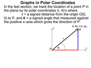
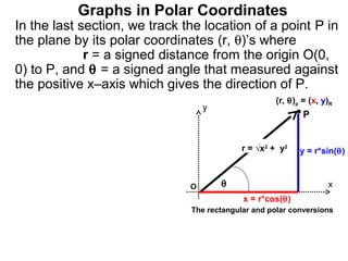
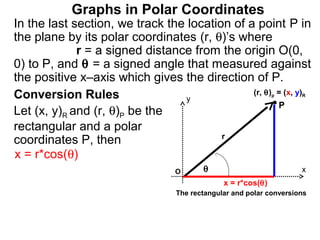
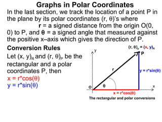
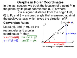
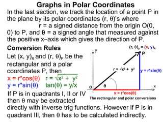
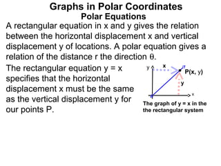
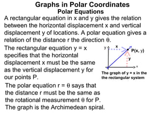
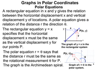
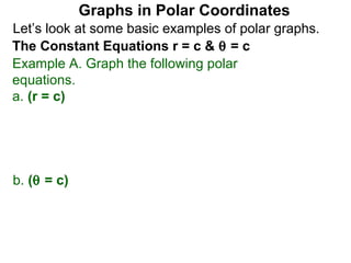
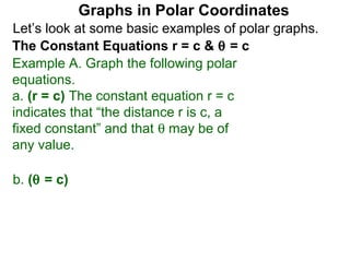
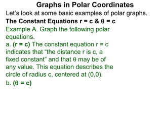
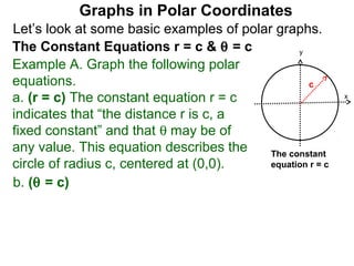
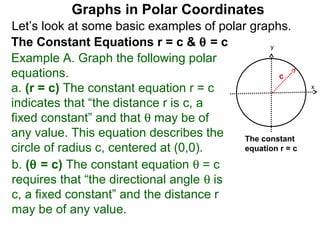
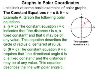
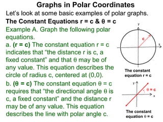
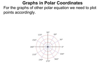
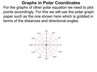
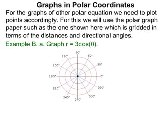
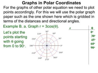
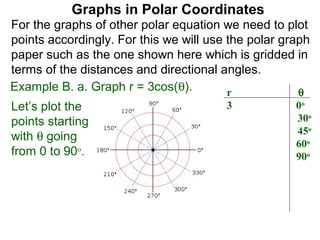
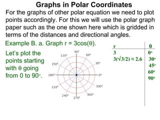
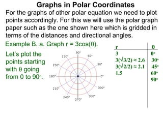
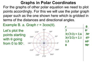
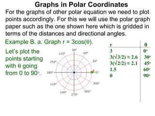
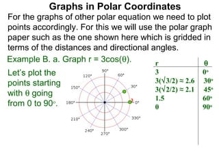
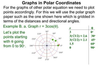
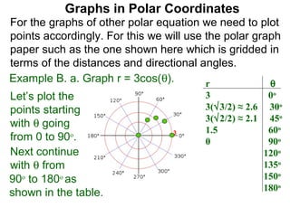
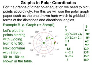
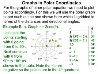
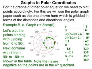
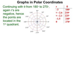
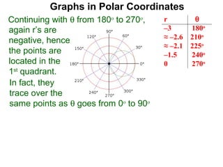
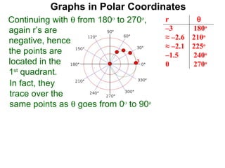
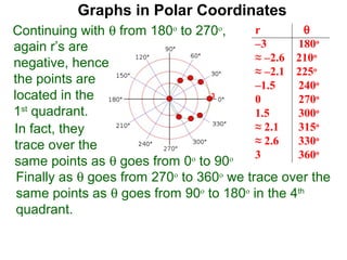
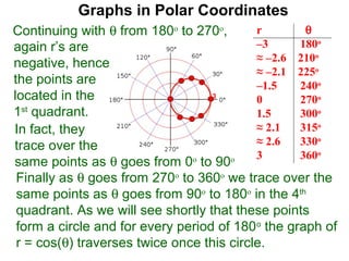
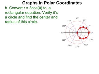
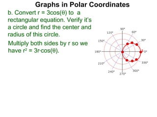
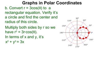
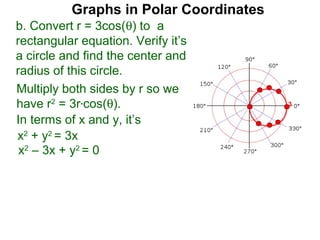
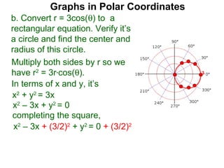
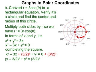
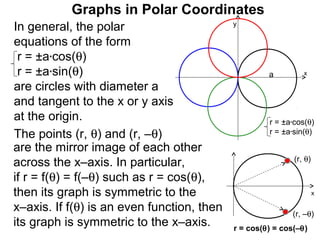
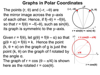
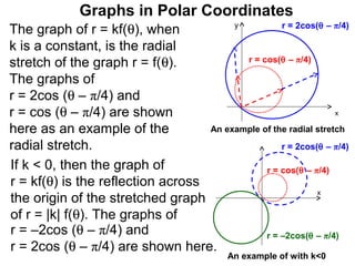
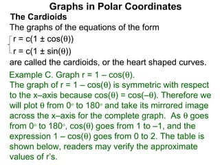
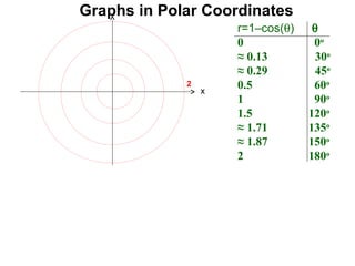
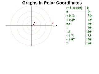
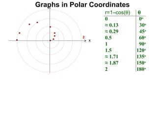
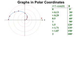
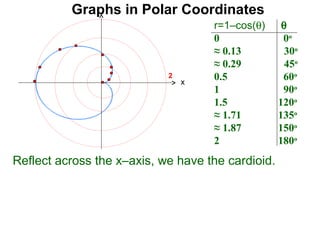
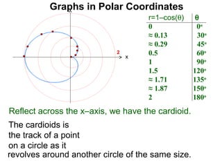
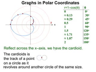
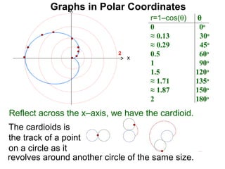
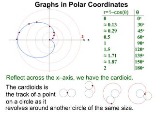
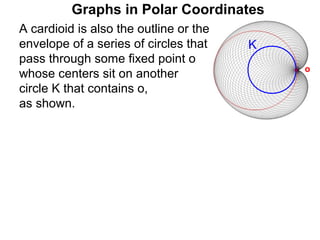
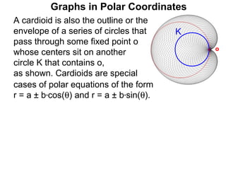
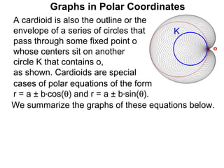
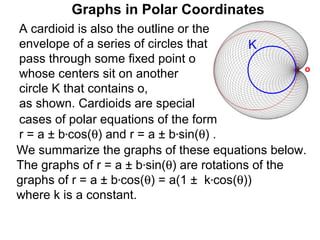
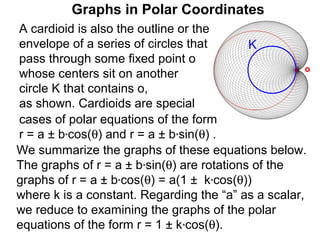
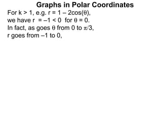
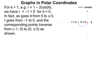
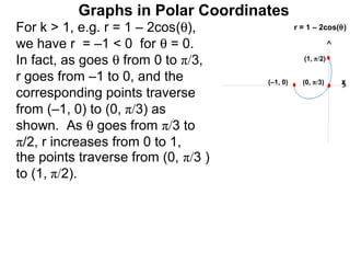
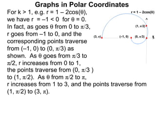
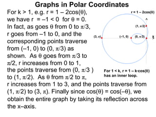
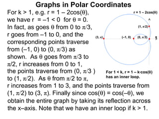
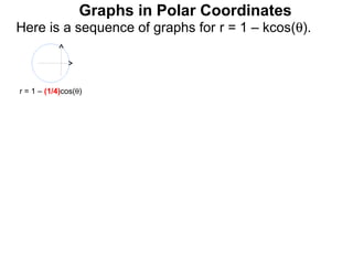
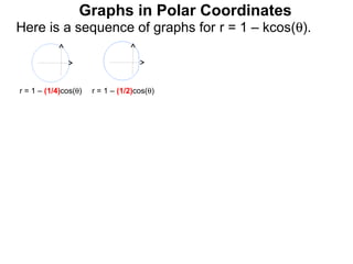
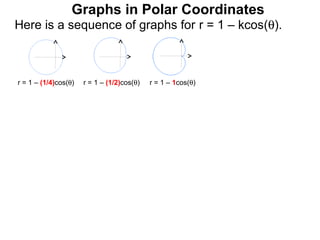
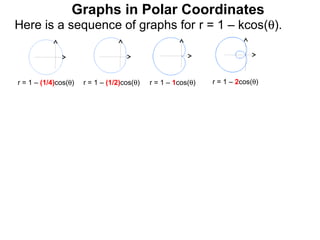
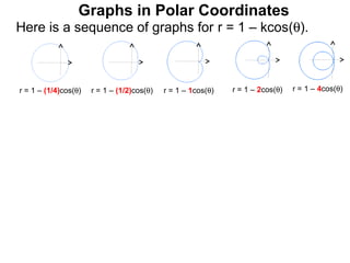
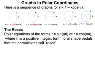
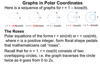
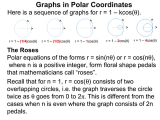
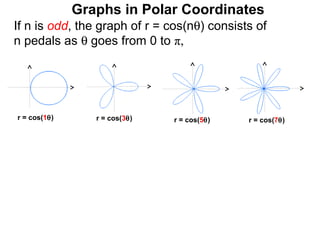
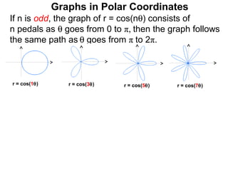
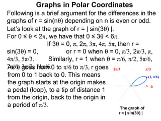
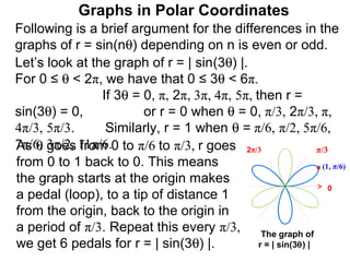
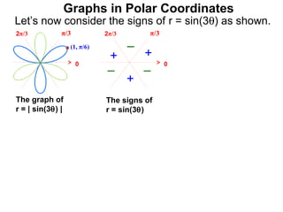
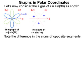
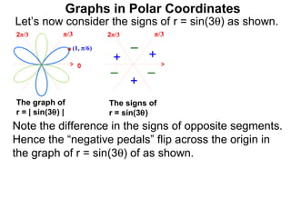
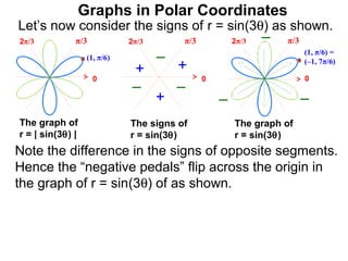
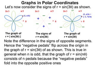
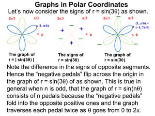
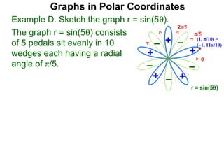
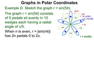
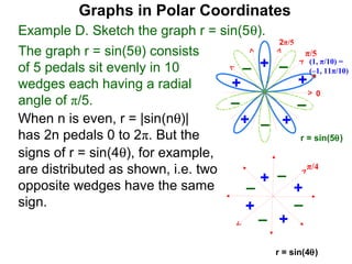
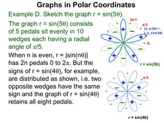
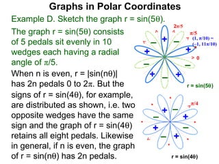
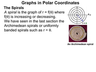
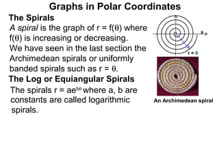
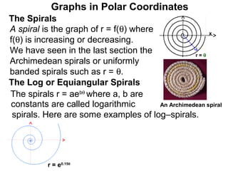
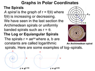
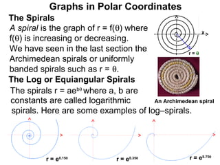
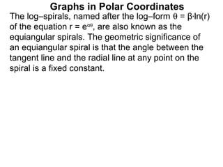
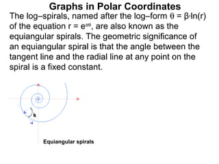
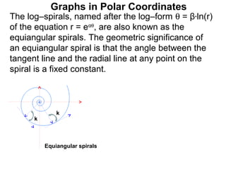
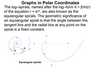
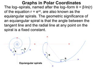
Graphs in Polar Coordinates
In the last section, we track the location of a point P in
the plane by its polar coordinates (r, θ)’s where
r = a signed distance from the origin O(0,
0) to P, and θ = a signed angle that measured against
the positive x–axis which gives the direction of P.
(r, θ)p = (x, y)R
y
P

r

O θ x

(r, θ)p = (x, y)R
y
P

r = √x2 + y2 y = r*sin(θ)

O θ x
x = r*cos(θ)
The rectangular and polar conversions

Conversion Rules (r, θ) = (x, y)
p R
y
P
Let (x, y)R and (r, θ)P be the
rectangular and a polar
r
coordinates P, then
x = r*cos(θ)
O θ x
x = r*cos(θ)

Conversion Rules (r, θ) = (x, y) p R
y
P
r
coordinates P, then y = r*sin(θ)

x = r*cos(θ)
y = r*sin(θ) O θ x
x = r*cos(θ)

Conversion Rules (r, θ) = (x, y)p R
y
P
r = √x + y 2 2

x = r*cos(θ) r = √x2 + y2
y = r*sin(θ) tan(θ) = y/x O θ x
x = r*cos(θ)

Conversion Rules (r, θ) = (x, y)
p R
y
P
r = √x + y2 2

x = r*cos(θ) r = √x2 + y2
y = r*sin(θ) tan(θ) = y/x O θ x

If P is in quadrants I, II or IV x = r*cos(θ)
then θ may be extracted
directly with inverse trig functions. However if P is in
quadrant IIl, then θ has to be calculated indirectly.

Polar Equations

Polar Equations
A rectangular equation in x and y gives the relation
between the horizontal displacement x and vertical
displacement y of locations.

Polar Equations
displacement y of locations. A polar equation gives a
relation of the distance r the direction θ.

Polar Equations
The rectangular equation y = x
specifies that the horizontal
displacement x must be the same
as the vertical displacement y for
our points P.

Polar Equations
x
The rectangular equation y = x y
P(x, y)
specifies that the horizontal y
displacement x must be the same x
as the vertical displacement y for The graph of y = x in the
our points P. the rectangular system

Polar Equations
x
P(x, y)

The polar equation r = θ says that
the distance r must be the same as
the rotational measurement θ for P.
The graph is the Archimedean spiral.

Polar Equations
x
P(x, y)

The polar equation r = θ says that P(r, θ)
the distance r must be the same as θ
r
the rotational measurement θ for P.
x
The graph is the Archimedean spiral. Graph of r = θ in the
polar system.

Let’s look at some basic examples of polar graphs.
The Constant Equations r = c & θ = c

Example A. Graph the following polar
equations.
a. (r = c)

b. (θ = c)

equations.
a. (r = c) The constant equation r = c
indicates that “the distance r is c, a
fixed constant” and that θ may be of
any value.

b. (θ = c)

equations.
a. (r = c) The constant equation r = c
any value. This equation describes the
circle of radius c, centered at (0,0).
b. (θ = c)

The Constant Equations r = c & θ = c y

equations. c
a. (r = c) The constant equation r = c x

any value. This equation describes the The constant
circle of radius c, centered at (0,0). equation r = c

b. (θ = c)


equations. c


b. (θ = c) The constant equation θ = c
requires that “the directional angle θ is
c, a fixed constant” and the distance r
may be of any value.


equations. c


b. (θ = c) The constant equation θ = c
may be of any value. This equation
describes the line with polar angle c.


equations. c


b. (θ = c) The constant equation θ = c y

θ=c
x
may be of any value. This equation
The constant
describes the line with polar angle c. equation θ = c

For the graphs of other polar equation we need to plot
points accordingly.

points accordingly. For this we will use the polar graph
paper such as the one shown here which is gridded in
terms of the distances and directional angles.

Example B. a. Graph r = 3cos(θ).

Example B. a. Graph r = 3cos(θ). r θ
Let’s plot the 3 0o
points starting 3(√3/2) ≈ 2.6 30o
3(√2/2) ≈ 2.1 45o
with θ going
1.5 60o
from 0 to 90o. 0 90o

3(√2/2) ≈ 2.1 45o
with θ going
3 1.5 60o

3(√2/2) ≈ 2.1 45o
with θ going
3 1.5 60o
Next continue –1.5 120o
with θ from ≈ –2.1 135o
90o to 180o as ≈ –2.6 150o
–3 180o
shown in the table.

3(√2/2) ≈ 2.1 45o
with θ going
3 1.5 60o
from 0 to 90 .
o
0 90o
Next continue –1.5 120o
with θ from ≈ –2.1 135o
90o to 180o as ≈ –2.6 150o
–3 180o
shown in the table. Note the r’s are
negative so the points are in the 4th quadrant.

Continuing with θ from 180o to 270o, r θ
again r’s are –3 180o
≈ –2.6 210o
negative, hence
≈ –2.1 225o
the points are –1.5 240o
located in the 0 270o
1st quadrant. 1.5 300o
≈ 2.1 315o
≈ 2.6 330o
3 360o

≈ –2.6 210o
negative, hence
≈ –2.1 225o
located in the 0 270o
In fact, they ≈ 2.1 315o
trace over the ≈ 2.6 330o
3 360o
same points as θ goes from 0o to 90o

≈ –2.6 210o
negative, hence
≈ –2.1 225o
located in the 3
0 270o
3 360o
same points as θ goes from 0o to 90o

≈ –2.6 210o
negative, hence
≈ –2.1 225o
located in the 3
0 270o
3 360o
same points as θ goes from 0 to 90
o o

Finally as θ goes from 270o to 360o we trace over the
same points as θ goes from 90o to 180o in the 4th
quadrant.

≈ –2.6 210o
negative, hence
≈ –2.1 225o
located in the 3
0 270o
3 360o
same points as θ goes from 0 to 90
o o

Finally as θ goes from 270o to 360o we trace over the
same points as θ goes from 90o to 180o in the 4th
quadrant. As we will see shortly that these points
form a circle and for every period of 180o the graph of
r = cos(θ) traverses twice once this circle.

b. Convert r = 3cos(θ) to a
rectangular equation. Verify it’s
a circle and find the center and
radius of this circle.

3

Multiply both sides by r so we
have r2 = 3r*cos(θ). 3


In terms of x and y, it’s
x2 + y2 = 3x


x2 + y2 = 3x
x2 – 3x + y2 = 0


x2 + y2 = 3x
x2 – 3x + y2 = 0
completing the square,
x2 – 3x + (3/2)2 + y2 = 0 + (3/2)2


x2 + y2 = 3x
x2 – 3x + y2 = 0
x2 – 3x + (3/2)2 + y2 = 0 + (3/2)2
(x – 3/2)2 + y2 = (3/2)2


x2 + y2 = 3x
x2 – 3x + y2 = 0
x2 – 3x + (3/2)2 + y2 = 0 + (3/2)2
(x – 3/2)2 + y2 = (3/2)2
so the points form the circle centers at (3/2, 0) with
radius 3/2.

In general, the polar y

equations of the form
r = ±a*cos(θ)
r = ±a*sin(θ) a x

are circles with diameter a
and tangent to the x or y axis
at the origin. r = ±a*cos(θ)
r = ±a*sin(θ)


r = ±a*cos(θ)
r = ±a*sin(θ) a x

The points (r, θ) and (r, –θ) r = ±a*sin(θ)

are the mirror image of each other
(r, θ)
across the x–axis.

x

(r, –θ)
r = cos(θ) = cos(–θ)


r = ±a*cos(θ)
r = ±a*sin(θ) a x


(r, θ)
across the x–axis. In particular,
if r = f(θ) = f(–θ) such as r = cos(θ),
then its graph is symmetric to the x

x–axis. (r, –θ)
r = cos(θ) = cos(–θ)


r = ±a*cos(θ)
r = ±a*sin(θ) a x


(r, θ)
across the x–axis. In particular,
if r = f(θ) = f(–θ) such as r = cos(θ),
then its graph is symmetric to the x

x–axis. If f(θ) is an even function, then (r, –θ)
its graph is symmetric to the x–axis. r = cos(θ) = cos(–θ)

y
The points (r, θ) and (–r, –θ) are (–r, –θ) (r, θ)

the mirror image across the y–axis
of each other. Hence, if f(–θ) = –f(θ),
so that r = f(θ) = –f(–θ), such as sin(θ),
x
its graph is symmetric to the y–axis. r = sin(θ) = –sin(–θ)

y
Given r = f(θ), let g(θ) = f(θ – α) so that r = cos(θ – π/4)

g(θ + α) = f(θ) = k. Hence the point
(k, θ + α) on the graph of g is just the
point (k, θ) on the graph of f rotated by π/4 x
the angle α.
The graph of r = cos (θ – π/4) is shown
r = cos(θ)
here as the rotated r = cos(θ).

y r = 2cos(θ – π/4)
The graph of r = kf(θ), when
k is a constant, is the radial
stretch of the graph r = f(θ). r = cos(θ – π/4)

The graphs of
r = 2cos (θ – π/4) and
r = cos (θ – π/4) are shown x

here as an example of the An example of the radial stretch
radial stretch. r = 2cos(θ – π/4)

If k < 0, then the graph of r = cos(θ – π/4)
r = kf(θ) is the reflection across
x
the origin of the stretched graph
of r = |k| f(θ). The graphs of
r = –2cos (θ – π/4) and r = –2cos(θ – π/4)
r = 2cos (θ – π/4) are shown here.
An example of with k<0

The Cardioids
The graphs of the equations of the form
r = c(1 ± cos(θ))
r = c(1 ± sin(θ))
are called the cardioids, or the heart shaped curves.
Example C. Graph r = 1 – cos(θ).
The graph of r = 1 – cos(θ) is symmetric with respect
to the x–axis because cos(θ) = cos(–θ). Therefore we
will plot θ from 0o to 180o and take its mirrored image
across the x–axis for the complete graph. As θ goes
from 0o to 180o, cos(θ) goes from 1 to –1, and the
expression 1 – cos(θ) goes from 0 to 2. The table is
shown below, readers may verify the approximate
values of r’s.

r=1–cos(θ) θ
0 0o
≈ 0.13 30o
≈ 0.29 45o
2
x
0.5 60o
1 90o
1.5 120o
≈ 1.71 135o
≈ 1.87 150o
2 180o

r=1–cos(θ) θ
0 0o
≈ 0.13 30o
≈ 0.29 45o
2
x
0.5 60o
1 90o
1.5 120o
≈ 1.71 135o
≈ 1.87 150o
2 180o
Reflect across the x–axis, we have the cardioid.

r=1–cos(θ) θ
0 0o
≈ 0.13 30o
≈ 0.29 45o
2
x
0.5 60o
1 90o
1.5 120o
≈ 1.71 135o
≈ 1.87 150o
2 180o
Reflect across the x–axis, we have the cardioid.
The cardioids is
the track of a point
on a circle as it
revolves around another circle of the same size.

A cardioid is also the outline or the
envelope of a series of circles that
pass through some fixed point o

o

o
whose centers sit on another
circle K that contains o,

envelope of a series of circles that K
o
as shown.

o
as shown. Cardioids are special
cases of polar equations of the form
r = a ± b*cos(θ) and r = a ± b*sin(θ).

o
r = a ± b*cos(θ) and r = a ± b*sin(θ).
We summarize the graphs of these equations below.

o
r = a ± b*cos(θ) and r = a ± b*sin(θ) .
The graphs of r = a ± b*sin(θ) are rotations of the
graphs of r = a ± b*cos(θ) = a(1 ± k*cos(θ))
where k is a constant.

o
r = a ± b*cos(θ) and r = a ± b*sin(θ) .
The graphs of r = a ± b*sin(θ) are rotations of the
graphs of r = a ± b*cos(θ) = a(1 ± k*cos(θ))
where k is a constant. Regarding the “a” as a scalar,
we reduce to examining the graphs of the polar
equations of the form r = 1 ± k*cos(θ).

The graph of a polar equation of the form
r = 1 ± k*cos(θ) depend on the value of |k|.

We may classify the graphs r = 1 – k*cos(θ) where k is
a positive number into to three types.

a positive number into to three types..
For k = 1, or r = 1 – cos(θ),
we get a cardioid.
r = 1 – cos(θ)
k=1

For k = 1, or r = 1 – cos(θ),
we get a cardioid.
r = 1 – cos(θ)
For k < 1, e.g. r = 1 – ½ *cos(θ), k=1

we have r > 0 for all θ’s.

For k = 1, or r = 1 – cos(θ),
we get a cardioid.
r = 1 – cos(θ)
For k < 1, e.g. r = 1 – ½ *cos(θ), k=1

This means the graph does not
pass the origin.

For k = 1, or r = 1 – cos(θ),
we get a cardioid.
r = 1 – cos(θ)
For k < 1, e.g. r = 1 – ½ *cos(θ), k=1

This means the graph does not
pass the origin. Instead, the
cusp, i.e. the pinched point at
the origin of the cardioid, r = 1 – k *cos(θ)
is pushed out as shown. 0<k<1

For k > 1, e.g. r = 1 – 2cos(θ),
we have r = –1 < 0 for θ = 0.

For k > 1, e.g. r = 1 – 2cos(θ),
we have r = –1 < 0 for θ = 0.
In fact, as goes θ from 0 to π/3,
r goes from –1 to 0,

For k > 1, e.g. r = 1 – 2cos(θ), r = 1 – 2cos(θ)

we have r = –1 < 0 for θ = 0.
In fact, as goes θ from 0 to π/3,
r goes from –1 to 0, and the (–1, 0) (0, π/3) x
corresponding points traverse
from (–1, 0) to (0, π/3) as
shown.


we have r = –1 < 0 for θ = 0.
In fact, as goes θ from 0 to π/3, (1, π/2)

r goes from –1 to 0, and the (–1, 0) (0, π/3) x
from (–1, 0) to (0, π/3) as
shown. As θ goes from π/3 to
π/2, r increases from 0 to 1,
the points traverse from (0, π/3 )
to (1, π/2).


we have r = –1 < 0 for θ = 0.

r goes from –1 to 0, and the (3, π) (–1, 0) (0, π/3) x
from (–1, 0) to (0, π/3) as
the points traverse from (0, π/3 )
to (1, π/2). As θ from π/2 to π,
r increases from 1 to 3, and the points traverse from
(1, π/2) to (3, π).


we have r = –1 < 0 for θ = 0.

from (–1, 0) to (0, π/3) as
the points traverse from (0, π/3 ) For 1 < k, r = 1 – k cos(θ)
*

to (1, π/2). As θ from π/2 to π, has an inner loop.

(1, π/2) to (3, π). Finally since cos(θ) = cos(–θ), we
obtain the entire graph by taking its reflection across
the x–axis.


we have r = –1 < 0 for θ = 0.

from (–1, 0) to (0, π/3) as
the points traverse from (0, π/3 ) For 1 < k, r = 1 – k cos(θ)
*

to (1, π/2). As θ from π/2 to π, has an inner loop.

(1, π/2) to (3, π). Finally since cos(θ) = cos(–θ), we
obtain the entire graph by taking its reflection across
the x–axis. Note that we have an inner loop if k > 1.

Here is a sequence of graphs for r = 1 – kcos(θ).

r = 1 – (1/4)cos(θ)


r = 1 – (1/4)cos(θ) r = 1 – (1/2)cos(θ)


r = 1 – (1/4)cos(θ) r = 1 – (1/2)cos(θ) r = 1 – 1cos(θ)


r = 1 – (1/4)cos(θ) r = 1 – (1/2)cos(θ) r = 1 – 1cos(θ) r = 1 – 2cos(θ)


r = 1 – (1/4)cos(θ) r = 1 – (1/2)cos(θ) r = 1 – 1cos(θ) r = 1 – 2cos(θ) r = 1 – 4cos(θ)



The Roses
Polar equations of the forms r = sin(nθ) or r = cos(nθ),
where n is a positive integer, form floral shape pedals
that mathematicians call “roses”.



The Roses
Recall that for n = 1, r = cos(θ) consists of two
overlapping circles, i.e. the graph traverses the circle
twice as θ goes from 0 to 2π.



The Roses
Recall that for n = 1, r = cos(θ) consists of two
overlapping circles, i.e. the graph traverses the circle
twice as θ goes from 0 to 2π. This is different from the
cases when n is even where the graph consists of 2n
pedals.

If n is odd, the graph of r = cos(nθ) consists of
n pedals as θ goes from 0 to π,

r = cos(1θ) r = cos(3θ) r = cos(5θ) r = cos(7θ)

n pedals as θ goes from 0 to π, then the graph follows
the same path as θ goes from π to 2π.




If n is even, the graph of r = cos(nθ) traces out
2n pedals as θ goes from 0 to 2π.

Following is a brief argument for the differences in the
graphs of r = sin(nθ) depending on n is even or odd.

Let’s look at the graph of r = | sin(3θ) |.

For 0 ≤ θ < 2π, we have that 0 ≤ 3θ < 6π.

If 3θ = 0, π, 2π, 3π, 4π, 5π, then r =
sin(3θ) = 0, or r = 0 when θ = 0, π/3, 2π/3, π,
4π/3, 5π/3
2π/3 π/3

0

The graph of
r = | sin(3θ) |

If 3θ = 0, π, 2π, 3π, 4π, 5π, then r =
4π/3, 5π/3. Similarly, r = 1 when θ = π/6, π/2, 5π/6,
7π/6, 3π/2, 11π/6. 2π/3 π/3

0

The graph of
r = | sin(3θ) |

If 3θ = 0, π, 2π, 3π, 4π, 5π, then r =
As θ goes from
7π/6, 3π/2, 11π/6.0 to π/6 to π/3, r goes 2π/3 π/3
from 0 to 1 back to 0.
0

The graph of
r = | sin(3θ) |

If 3θ = 0, π, 2π, 3π, 4π, 5π, then r =
As θ goes from
from 0 to 1 back to 0. This means (1, π/6)
the graph starts at the origin makes
0
a pedal (loop), to a tip of distance 1
from the origin, back to the origin in
a period of π/3. The graph of
r = | sin(3θ) |

If 3θ = 0, π, 2π, 3π, 4π, 5π, then r =
As θ goes from
from 0 to 1 back to 0. This means (1, π/6)
the graph starts at the origin makes
0
a pedal (loop), to a tip of distance 1
from the origin, back to the origin in
a period of π/3. Repeat this every π/3, The graph of
we get 6 pedals for r = | sin(3θ) |. r = | sin(3θ) |

Let’s now consider the signs of r = sin(3θ) as shown.
below. π/3
2π/3 2π/3 π/3
(1, π/6) –
+ +
0 0
– –
+
The graph of The signs of
r = | sin(3θ) | r = sin(3θ)

below. π/3
2π/3 2π/3 π/3
(1, π/6) –
+ +
0 0
– –
+
r = | sin(3θ) | r = sin(3θ)
Note the difference in the signs of opposite segments.

below. π/3
2π/3 2π/3 π/3
(1, π/6) –
+ +
0
– –
+
r = | sin(3θ) | r = sin(3θ)
Hence the “negative pedals” flip across the origin in
the graph of r = sin(3θ) of as shown.

below. π/3
2π/3 2π/3 π/3 2π/3 – π/3
(1, π/6) – (1, π/6) =

+ + (–1, 7π/6)

0 0 0
– –
+ – –
The graph of The signs of The graph of
r = | sin(3θ) | r = sin(3θ) r = sin(3θ)
the graph of r = sin(3θ) of as shown.

below. π/3
2π/3 2π/3 π/3 2π/3 – π/3
(1, π/6) – (1, π/6) =

+ + (–1, 7π/6)

0 0 0
– –
+ – –
the graph of r = sin(3θ) of as shown. This is true in
general when n is odd, that the graph of r = sin(nθ)
consists of n pedals because the “negative pedals”
fold into the opposite positive ones

below. π/3
2π/3 2π/3 π/3 2π/3 – π/3
(1, π/6) – (1, π/6) =

+ + (–1, 7π/6)

0 0 0
– –
+ – –
the graph of r = sin(3θ) of as shown. This is true in
general when n is odd, that the graph of r = sin(nθ)
consists of n pedals because the “negative pedals”
fold into the opposite positive ones and the graph
traverses each pedal twice as θ goes from 0 to 2π.

Example D. Sketch the graph r = sin(5θ).

The graph r = sin(5θ) consists
of 5 pedals sit evenly in 10
wedges each having a radial
angle of π/5.

2π/5
The graph r = sin(5θ) consists π/5
of 5 pedals sit evenly in 10
0
angle of π/5.

r = sin(5θ)

2π/5
(1, π/10) =
of 5 pedals sit evenly in 10 (–1, 11π/10)
0
angle of π/5.

r = sin(5θ)

2π/5
of 5 pedals sit evenly in 10 – + – (1, π/10) =
(–1, 11π/10)
wedges each having a radial + +
0
angle of π/5. – –
+ – +
r = sin(5θ)

2π/5
(–1, 11π/10)
0
When n is even, r = |sin(nθ)| + – +
has 2n pedals 0 to 2π. r = sin(5θ)

2π/5
(–1, 11π/10)
0
has 2n pedals 0 to 2π. But the r = sin(5θ)
signs of r = sin(4θ), for example,
are distributed as shown, i.e. two π/4

opposite wedges have the same
+ –
– +
sign. + –
– +
r = sin(4θ)

2π/5
– +
(1, π/10) =
of 5 pedals sit evenly in 10 – (–1, 11π/10)
0
+ –
opposite wedges have the same – +
sign and the graph of r = sin(4θ) + –
retains all eight pedals. – +
r = sin(4θ)

2π/5
– +
(1, π/10) =
of 5 pedals sit evenly in 10 – (–1, 11π/10)
0
+ –
opposite wedges have the same – +
sign and the graph of r = sin(4θ) + –
retains all eight pedals. Likewise – +
in general, if n is even, the graph
of r = sin(nθ) has 2n pedals. r = sin(4θ)

The Spirals
A spiral is the graph of r = f(θ) where
f(θ) is increasing or decreasing.

The Spirals
A spiral is the graph of r = f(θ) where x
We have seen in the last section the r=θ
Archimedean spirals or uniformly
banded spirals such as r = θ.

An Archimedean spiral

The Spirals
The Log or Equiangular Spirals
The spirals r = aebθ where a, b are
constants are called logarithmic An Archimedean spiral
spirals.

The Spirals
spirals. Here are some examples of log–spirals.

r = e0.15θ

The Spirals

r = e0.15θ r = e0.35θ

The Spirals

r = e0.15θ r = e0.35θ r = e0.75θ

The log–spirals, named after the log–form θ = β*ln(r)
of the equation r = eαθ, are also known as the
equiangular spirals.

equiangular spirals. The geometric significance of
an equiangular spiral is that the angle between the
tangent line and the radial line at any point on the
spiral is a fixed constant.


k

Equiangular spirals


k
k

Equiangular spirals


k
k
q
q

Equiangular spirals


http://en.wikipedia.
org/wiki/Logarithmi
c_spiral

Equiangular spirals occur in nature frequently.


org/wiki/Logarithmi
c_spiral

In many biological growth processes, the new growth
is extruded at a fixed angle from the existing mass–
such as the generation of new sea shell along the
edge of the old shell.


org/wiki/Logarithmi
c_spiral

In many biological growth processes, the new growth
is extruded at a fixed angle from the existing mass,
e.g. the generation of new sea shell along the edge of
the old shell. Overtime the equiangular–spiral growth
lines emerge.

2 polar graphs

More Related Content

What's hot

Similar to 2 polar graphs

2 polar graphs