3 classification

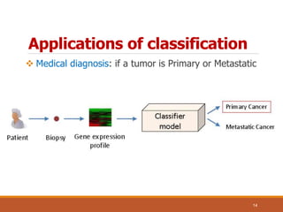
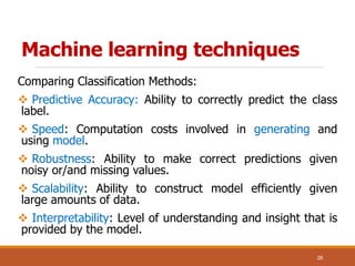
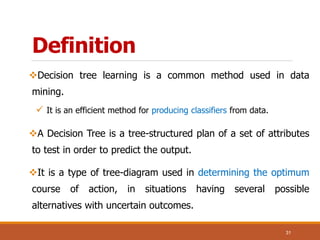
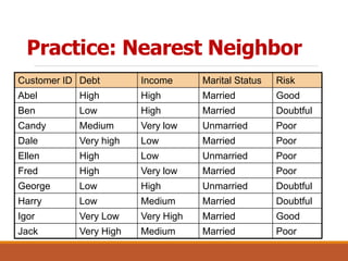
Classifications
Mahmoud Rafeek Alfarra
http://mfarra.cst.ps
University College of Science & Technology- Khan yonis
Development of computer systems
2016
Chapter 3 – Lecture 1

Outline
Definition of classification
Basic principles of classification
Typical applications of classification
How Does Classification Works?
Difference between Classification & Prediction.
 Machine learning techniques
 Decision Trees
 k-Nearest Neighbors
2

Definition
 Classification is: Techniques used to predict group
membership for data instances.
 Classification is: a data mining function that assigns items
in a collection to target categories or classes.
 The goal of classification is to accurately predict the target
class for each case in the data.

Definition
For example:
 Identify loan applicants as low, medium, or high credit risks.
 A bank loan officer wants to analyze the data in order to know
which customer (loan applicant) are risky or which are safe.
A marketing manager at a company needs to analyze a
customer with a given profile, who will buy a new computer.
4

Definition
 This type of learning called supervised learning
8

Basic principles of classification
9
Want to classify objects as boats and houses

10
 All objects before the coast line are boats and all objects after the coast
line are houses.
 Coast line serves as a decision surface that separates two classes.

11
 The methods that build classification models (i.e., “classification algorithms”)
operate very similarly to the previous example.
 First all objects are represented geometrically.

12
Then the algorithm seeks to find a decision surface that
separates classes of objects .

13
Unseen (new) objects are classified as “boats” if they fall
below the decision surface and as “houses” if the fall above it.

Applications of classification
 Medical diagnosis: if a tumor is Primary or Metastatic
14

Credit/loan approval.
Fraud detection: if a transaction is fraudulent
Web page categorization: which category it is
Classifying secondary structures of protein
as alpha-helix, beta-sheet, or random
coil
Categorizing news stories as finance, weather,
entertainment, sports, etc
15
Applications of classification

Classifications
2016

Outline
 Definition of classification
 Basic principles of classification
 Typical applications of classification
 How Does Classification Works?
 Difference between Classification & Prediction.
 Decision Trees
17

How Does Classification Works?
The Data Classification process includes two steps:
 Building the Classifier or Model
 Using Classifier for Classification
18

19

Given a collection of records (training set )
Each record contains a set of attributes, one of the
attributes is the class.
Find a model for class attribute as a function of the
values of other attributes.
Goal: previously unseen records should be assigned a
class as accurately as possible.
A test set is used to determine the accuracy of the
model.
Usually, the given data set is divided into training and
test sets, with training set used to build the model and
test set used to validate it.
20

21
Training
Data
NAME RANK YEARS TENURED
Mike Assistant Prof 3 no
Mary Assistant Prof 7 yes
Bill Professor 2 yes
Jim Associate Prof 7 yes
Dave Assistant Prof 6 no
Anne Associate Prof 3 no
Classification
Algorithms
IF rank = ‘professor’
OR years > 6
THEN tenured = ‘yes’
Classifier
(Model)
Process 1 Model Construction: example

22
Classifier
Testing
Data
NAME RANK YEARS TENURED
Tom Assistant Prof 2 no
Merlisa Associate Prof 7 no
George Professor 5 yes
Joseph Assistant Prof 7 yes
Unseen Data
(Jeff, Professor, 4)
Tenured?
Process 2 Using the Model in Prediction

Difference between
Classification & Prediction
Classification
 Has prior knowledge
about class.
A model or a classifier will
be constructed that predicts
the class of unseen object.
Prediction
 Has prior knowledge
about class.
 A model or a predictor
will be constructed that
predicts a continuous-
valued-function or ordered
value.
23

Difference between
Classification & Prediction
If you use a classification model to predict the
treatment outcome for a new patient, it would be
a prediction.
 In the book "Data Mining Concepts and
Techniques", Han and Kamber's view is that
predicting class labels is classification, and
predicting values is prediction.
24

Machine learning techniques
 Learning: Things learn when they change their behavior in a
way that makes them perform better in the future.
 Machine learning: is the subfield of artificial intelligence that
is concerned with the design and development of algorithms
that allow computers (machines) to improve their performance
over time (to learn) based on data, such as from sensor data or
databases.

Comparing Classification Methods:
 Predictive Accuracy: Ability to correctly predict the class
label.
 Speed: Computation costs involved in generating and
using model.
 Robustness: Ability to make correct predictions given
noisy or/and missing values.
 Scalability: Ability to construct model efficiently given
large amounts of data.
 Interpretability: Level of understanding and insight that is
provided by the model.
26

Examples of machine learning techniques:
Decision Trees
Rule Induction
k-Nearest Neighbors
Naïve Bayesian Classifiers
Neural Network
27

Classifications
Decision Trees
2016

Outline
 Decision Trees
29

Outline
 Definition
 Decision tree consist of …
 Decision Tree Classification Task
 Apply Model to Test Data
 Building Tree
 A criterion for attribute selection
 Decision Tree to Decision Rules
30

Definition
Decision tree learning is a common method used in data
mining.
 It is an efficient method for producing classifiers from data.
A Decision Tree is a tree-structured plan of a set of attributes
to test in order to predict the output.
It is a type of tree-diagram used in determining the optimum
course of action, in situations having several possible
alternatives with uncertain outcomes.
31

Decision Trees: Definition
Decision tree consist of:
An internal node is a test on an attribute, e.g. Body temperature .
A branch represents an outcome of the test, e.g., Warm
A leaf node represents a class label e.g. Mammals
At each node, one attribute is chosen to split training examples
into distinct classes as much as possible
A new case is classified by following a matching path to a leaf
node.
36

Example of a Decision Tree
Tid Refund Marital
Status
Taxable
Income Cheat
1 Yes Single 125K No
2 No Married 100K No
3 No Single 70K No
4 Yes Married 120K No
5 No Divorced 95K Yes
6 No Married 60K No
7 Yes Divorced 220K No
8 No Single 85K Yes
9 No Married 75K No
10 No Single 90K Yes
10
Refund
MarSt
TaxInc
YESNO
NO
NO
Yes No
MarriedSingle, Divorced
< 80K > 80K
Splitting Attributes
Training Data Model: Decision Tree

Another Example of Decision Tree
Tid Refund Marital
Status
Taxable
Income Cheat
1 Yes Single 125K No
2 No Married 100K No
3 No Single 70K No
4 Yes Married 120K No
5 No Divorced 95K Yes
6 No Married 60K No
7 Yes Divorced 220K No
8 No Single 85K Yes
9 No Married 75K No
10 No Single 90K Yes
10
MarSt
Refund
TaxInc
YESNO
NO
NO
Yes No
Married
Single,
Divorced
< 80K > 80K
There could be more than one tree that fits
the same data!

Decision Tree Classification Task
Apply
Model
Induction
Deduction
Learn
Model
Model
Tid Attrib1 Attrib2 Attrib3 Class
1 Yes Large 125K No
2 No Medium 100K No
3 No Small 70K No
4 Yes Medium 120K No
5 No Large 95K Yes
6 No Medium 60K No
7 Yes Large 220K No
8 No Small 85K Yes
9 No Medium 75K No
10 No Small 90K Yes
10
Tid Attrib1 Attrib2 Attrib3 Class
11 No Small 55K ?
12 Yes Medium 80K ?
13 Yes Large 110K ?
14 No Small 95K ?
15 No Large 67K ?
10
Test Set
Tree
Induction
algorithm
Training Set
Decision Tree

Apply Model to Test Data
Refund
MarSt
TaxInc
YESNO
NO
NO
Yes No
< 80K > 80K
Refund Marital
Status
Taxable
Income Cheat
No Married 80K ?
10
Test Data
Start from the root of tree.

Refund
MarSt
TaxInc
YESNO
NO
NO
Yes No
< 80K > 80K
Refund Marital
Status
Taxable
Income Cheat
No Married 80K ?
10
Test Data

Refund
MarSt
TaxInc
YESNO
NO
NO
Yes No
< 80K > 80K
Refund Marital
Status
Taxable
Income Cheat
No Married 80K ?
10
Test Data
Assign Cheat to “No”

Decision Trees: Building Tree
There is a large number of decision-tree induction
algorithms described primarily in the machine-learning
and applied-statistics literature.
 They are supervised learning methods that construct
decision trees from a set of input-output samples.
Optimal tree is the smallest.
47

There is a large number of decision-tree induction
algorithms described primarily in the machine-learning
and applied-statistics literature.
 They are supervised learning methods that construct
decision trees from a set of input-output samples.
Optimal tree is the smallest.
48

Top-down tree construction
◦ At start, all training examples are at the root.
◦ Partition the examples recursively by choosing one
attribute each time.
49

Top-Down Induction of Decision Trees (Greedy Tree Growing)
Recursive Partitioning
◦ find “best” attribute test to install at root
◦ split data on root test
◦ find “best” attribute test to install at each new node
◦ split data on new test
◦ repeat until:
◦ all nodes are pure
◦ all nodes contain fewer than k cases
◦ tree reaches predetermined max depth
◦ no more attributes to test
50

Find “best” attribute test to install at root
Outlook Temperature Humidity Windy Play?
sunny hot high false No
sunny hot high true No
overcast hot high false Yes
rain mild high false Yes
rain cool normal false Yes
rain cool normal true No
overcast cool normal true Yes
sunny mild high false No
sunny cool normal false Yes
rain mild normal false Yes
sunny mild normal true Yes
overcast mild high true Yes
overcast hot normal false Yes
rain mild high true No
Decision Trees: Example

Decision Trees: Example
Overcast it
does not
need split
because it’s
need yes

A criterion for attribute selection
Which is the best attribute?
◦ The one which will result in the smallest tree
◦ Heuristic: choose the attribute that produces the “purest”
nodes
Popular impurity criterion: information gain
◦ Information gain increases with the average purity of the
subsets that an attribute produces
Strategy: choose attribute that results in greatest information
gain
53

Decision Tree to Decision Rules
A decision tree can easily be transformed to a set of rules
by mapping from the root node to the leaf nodes one by
one.
54

Decision Tree to Decision Rules
55

Practice: Draw decision tree using
the following instances:
56
Weekend Weather Parents Money
Decision
(Category)
W1 Sunny Yes Rich Cinema
W2 Sunny No Rich Tennis
W3 Windy Yes Rich Cinema
W4 Rainy Yes Poor Cinema
W5 Rainy No Rich Stay in
W7 Windy No Poor Cinema
W8 Windy No Rich Shopping

Practice: Convert the following to
Decision Rules
57
Decision
(Category)
D1 Sunny Yes Rich Cinema
W5 Rainy No Rich Stay in
W7 Windy No Poor Cinema
W8 Windy No Rich Shopping

Practice: Classify the following
instances:
58
Decision
(Category)
W11 Rainy Yes Rich ?
W12 Windy No Poor ?
W13 Sunny No Poor ?
W14 Windy Yes Poor ?
W15 Rainy No Poor ?

Practice: Again using the following
59

Classifications
k-Nearest Neighbors
2016

Outline
 Decision Trees
61

Definition: K-Nearest Neighbor
K-nearest neighbor is a supervised learning algorithm.
 A case is classified by a majority vote of its neighbors, with the
case being assigned to the class most common amongst its K
nearest neighbors measured by a distance function.
If K = 1, then the case is simply assigned to the class of its nearest
neighbor.
 The purpose of this algorithm is to classify a new object based on
attributes and training samples.
Also called instance based learning.
62

Definition: K-Nearest Neighbor
63

K-Nearest Neighbor Algorithm
Given a new instance x,
find its nearest neighbor <x’,y’>
Return y’ as the class of x
64

K-Nearest Neighbor: Example
A simple example of the nearest neighbor prediction
algorithm is that if you look at the people in your
neighborhood you may notice that, in general, you all have
similar incomes.
 So if your neighbors have an income greater than
$50,000, you have a chance to have a high income as well.
65

K-Nearest NeighborAlgorithm


n
i
ii yxYXd
1
2
)(),(
66
All instances correspond to points in the n-D space.
The nearest neighbor are defined in terms of Euclidean
distance.
Euclidean distance between two points , X=(x1,x2,…,xn) and
Y=(y1,y2,…yn) is:

Here is step by step on how to compute K-nearest
neighbors KNN algorithm:
1) Determine parameter K = number of nearest
neighbors
2) Calculate the distance between the query-instance
and all the training samples
3) Sort the distance and determine nearest neighbors
based on the K-th minimum distance
4) Gather the category of the nearest neighbors
5) Use simple majority of the category of nearest
neighbors as the prediction value of the query instance
67

68

69
Using the standardized
distance on the same
training set, the
unknown case
returned a different
neighbor which is not
a good sign of
robustness.

Example
X1 X2 Y
7 7 Bad
7 4 Bad
3 4 Good
1 4 Good
70
We have data from the
questionnaires survey here is
four training samples :
test with X1 = 3 and X2 = 7

Example
X1 X2 Distance
7 7 (7-3)2+(7-7)2=16
7 4 (7-3)2+(4-7)2=25
3 4 (3-3)2+(4-7)2=9
1 4 (1-3)2+(4-7)2=13
71
1. Suppose use K = 3
2. Calculate the distance between the query-instance and
all the training samples

Example
X1 X2 Distance Rank
7 7 (7-3)2+(7-7)2=16 3
7 4 (7-3)2+(4-7)2=25 4
3 4 (3-3)2+(4-7)2=9 1
1 4 (1-4)2+(4-7)2=13 2
72
3. Sort the distance and determine nearest neighbors based
on the K-th minimum distance

Example
X1 X2 Distance Rank Y
7 7 (7-3)2-(7-7)2=16 3 Bad
7 4 (7-3)2-(4-7)2=25 4 -
3 4 (3-3)2-(4-7)2=9 1 Good
1 4 (1-4)2-(4-7)2=13 2 Good
73
4. Gather the category of the nearest neighbors. Notice in the
second row last column that the category of nearest neighbor
(Y) is not included because the rank of this data is more than
3 (=K).

Example
5) Use simple majority of the category of nearest
neighbors as the prediction value of the query instance
We have 2 good and 1 bad, since 2>1 then we conclude
that a new test with X1 = 3 and X2 = 7 is included in
Good category.
74

Scaling issues
◦ Attributes may have to be scaled to prevent distance
measures from being dominated by one of the
attributes
◦ Example:
◦ height of a person may vary from 1.5m to 1.8m
◦ weight of a person may vary from 90lb to 300lb
◦ income of a person may vary from $10K to $1M
Solution: Normalize the vectors to unit length (make
all values between 0 and 1).

Strength and Weakness
Advantage
◦ Robust to noisy training data
◦ Effective if the training data is large
Disadvantage
◦ Need to determine value of parameter K (number of nearest
neighbors)
◦ Distance based learning is not clear which type of distance to
use and which attribute to use to produce the best results. Shall
we use all attributes or certain attributes only?
◦ Computation cost is quite high because we need to compute
distance of each query instance to all training samples.
76

Lazy learning (e.g. nearest Neighbor):
Simply stores training data (or only minor processing) and
waits until it is given a test tuple
less time in training but more time in predicting
Eager learning (e.g. Decision tree and neural network):
Given a set of training set, constructs a classification model
before receiving new (e.g., test) data to classify
77
Lazy vs. eager learning

Practice: Nearest Neighbor
Customer ID Debt Income Marital Status Risk
Abel High High Married Good
Ben Low High Married Doubtful
Candy Medium Very low Unmarried Poor
Dale Very high Low Married Poor
Ellen High Low Unmarried Poor
Fred High Very low Married Poor
George Low High Unmarried Doubtful
Harry Low Medium Married Doubtful
Igor Very Low Very High Married Good
Jack Very High Medium Married Poor

Customer ID Debt Income Marital Sta. Risk Distance
Abel High High Married Good
Ben Low High Married Doubtful
Candy Medium Very low Unmarried Poor
Dale Very high Low Married Poor
Ellen High Low Unmarried Poor
Fred High Very low Married Poor
George Low High Unmarried Doubtful
Harry Low Medium Married Doubtful
Igor Very Low Very High Married Good
Jack Very High Medium Married Poor

Customer ID Debt Income Marital Status Risk
Zeb High Medium Married ?

3 classification

Recommended

Recommended

More Related Content

What's hot

What's hot (20)

Similar to 3 classification

Similar to 3 classification (20)

More from Mahmoud Alfarra

More from Mahmoud Alfarra (20)

Recently uploaded

Recently uploaded (20)

3 classification