The document discusses the use of the Random Forest algorithm in digital soil mapping (DSM) and modeling, particularly its application in regression and classification tasks. It provides examples of how to implement the model in R using the randomForest package, including data splitting, model fitting, and diagnostics. The final output includes predicting soil organic carbon maps for Macedonia, demonstrating the model's practical application.

1. Yusuf YIGINI, PhD - FAO, Land and Water Division (CBL)
GSP - Eurasian Soil
Partnership - Dijital
Toprak Haritalama ve
Modelleme Egitimi
Izmir, Turkiye
21-25 Agustos 2017

2. Random Forest

3. Random Forest
An increasingly popular data mining algorithm in
DSM and soil sciences, and even in applied sciences
in general is the Random Forests model. This
algorithm is provided in the randomForest package
and can be used for both regression and
classification.

4. Random Forest
Random Forests are a boosted decision tree model.
Fitting a Random Forest model in R is relatively
straightforward. It is better consulting the rhelp
files regarding the randomForest package and the
functions.

5. Random Forest
We will use the randomForest() function and a couple of
extractor functions to tease out some of the model fitting
diagnostics. We will use the sample() function to
randomly split the data into two parts: training and
testing.
> DSM_table2 <- read.csv("DSM_table2.csv")
> training <- sample(nrow(DSM_table2), 0.7 * nrow(DSM_table2))
> modelF <- randomForest(Value ~ dem + twi + slp + tmpd + tmpn, data =
DSM_table2[training, ],importance = TRUE, ntree = 1000)

6. Random Forest
The print function is to quickly assess the model fit.
print(modelF)
Call:
randomForest(formula = Value ~ dem + twi + slp + tmpd + tmpn,
data = DSM_table2[training, ], importance = TRUE, ntree = 1000)
Type of random forest: regression
Number of trees: 1000
No. of variables tried at each split: 1
Mean of squared residuals: 1.801046
% Var explained: 59.35

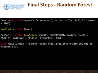
7. Random Forest
Generally, we confront this question by comparing
observed values with their predictions. Some of the more
common “quality” measures are the root mean square
error (RMSE), bias, and the R2 value
> Predicted <- predict(modelF, newdata = DSM_table2[-
training, ])
> RMSE <- sqrt(mean((DSM_table2$Value[-training] - Predicted)^2))
> RMSE
[1] 1.249491
> lm <- lm(Predicted~ DSM_table2$Value[-training])
> summary(lm)[["r.squared"]]
[1] 0.6079515
> bias <- mean(Predicted) - mean(DSM_table2$Value[-training])
> bias
[1] 0.01450241

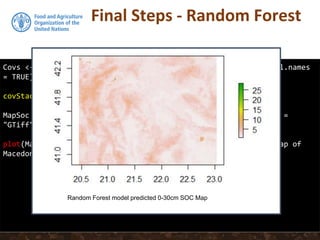
8. Random Forest
plot(DSM_table2$Value[-training],Predicted)
abline(a=0,b=1,lty=2, col="red")
abline(lm, col="blue")

9. Random Forest
plot(DSM_table2$Value[-training],Predicted)
abline(a=0,b=1,lty=2, col="red")
abline(lm, col="blue")
regression on predicted and observed values - blue
1:1 comparison - red

10. Final Steps - Random Forest
Covs <- list.files(path = "C:/mc/covs", pattern = ".tif$",full.names
= TRUE)
covStack <- stack(Covs)
MapSoc <- predict(covStack, modelF, "SOCMAPofMAcedonia", format =
"GTiff", datatype = "FLT4S", overwrite = TRUE)
plot(MapSoc, main = "Random Forest model predicted 0-30cm SOC Map of
Macedonia %")

11. Final Steps - Random Forest
Covs <- list.files(path = "C:/mc/covs", pattern = ".tif$",full.names
= TRUE)
covStack <- stack(Covs)
MapSoc <- predict(covStack, modelF, "SOCMAPofMAcedonia", format =
"GTiff", datatype = "FLT4S", overwrite = TRUE)
plot(MapSoc, main = "Random Forest model predicted 0-30cm SOC Map of
Macedonia %")
Random Forest model predicted 0-30cm SOC Map