Downloaded 21 times


![[Hastie et all., 2005]](https://image.slidesharecdn.com/talk4-151222141843/75/Conistency-of-random-forests-5-2048.jpg)

![Bagging
[Random Forest]](https://image.slidesharecdn.com/talk4-151222141843/75/Conistency-of-random-forests-7-2048.jpg)
![Grow different trees from same learning set ℒ 𝑛
Sampling with replacement [Breiman, 1994]
Random subspace sampling [Ho, 1995 & 1998]
Random output sampling [Breiman, 1998]
Randomized C4.5 [Dietterich, 1998]
Purely random forest [Breiman, 2000]
Extremely random trees [Guerts, 2006]](https://image.slidesharecdn.com/talk4-151222141843/75/Conistency-of-random-forests-13-2048.jpg)
![Grow different trees from same learning set ℒ 𝑛
Sampling with replacement - random subspace [Breiman, 2001]
Sampling with replacement - weighted subspace [Amaratunga, 2008; Xu,
2008; Wu, 2012]
Sampling with replacement - random subspace and regularized [Deng,
2012]
Sampling with replacement - random subspace and guided-regularized
[Deng, 2013]
Sampling with replacement - random subspace and random split
position selection [Saïp Ciss, 2014]](https://image.slidesharecdn.com/talk4-151222141843/75/Conistency-of-random-forests-14-2048.jpg)
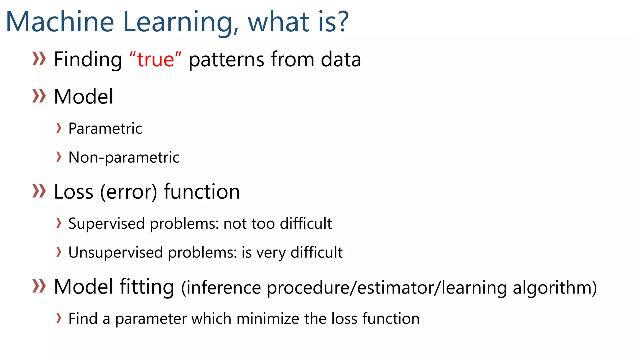
![What is a good learner?
[What is friendly with my data?]](https://image.slidesharecdn.com/talk4-151222141843/75/Conistency-of-random-forests-16-2048.jpg)
![Random Forest [Breiman, 2001]](https://image.slidesharecdn.com/talk4-151222141843/75/Conistency-of-random-forests-20-2048.jpg)
![WSRF [Wu, 2012]](https://image.slidesharecdn.com/talk4-151222141843/75/Conistency-of-random-forests-21-2048.jpg)
![Random Uniform Forest [Saïp Ciss, 2014]](https://image.slidesharecdn.com/talk4-151222141843/75/Conistency-of-random-forests-22-2048.jpg)
![RRF [Deng, 2012]](https://image.slidesharecdn.com/talk4-151222141843/75/Conistency-of-random-forests-23-2048.jpg)
![GRRF [Deng, 2013]](https://image.slidesharecdn.com/talk4-151222141843/75/Conistency-of-random-forests-24-2048.jpg)

![Random Forest [Breiman, 2001]](https://image.slidesharecdn.com/talk4-151222141843/75/Conistency-of-random-forests-27-2048.jpg)
![WSRF [Wu, 2012]](https://image.slidesharecdn.com/talk4-151222141843/75/Conistency-of-random-forests-28-2048.jpg)
![Random Uniform Forest [Saïp Ciss, 2014]](https://image.slidesharecdn.com/talk4-151222141843/75/Conistency-of-random-forests-29-2048.jpg)
![RRF [Deng, 2012]](https://image.slidesharecdn.com/talk4-151222141843/75/Conistency-of-random-forests-30-2048.jpg)
![GRRF [Deng, 2013]](https://image.slidesharecdn.com/talk4-151222141843/75/Conistency-of-random-forests-31-2048.jpg)
![GRRF with AUC [Deng, 2013]](https://image.slidesharecdn.com/talk4-151222141843/75/Conistency-of-random-forests-32-2048.jpg)
![GRRF with ER [Deng, 2013]](https://image.slidesharecdn.com/talk4-151222141843/75/Conistency-of-random-forests-33-2048.jpg)
![Random Forest [Breiman, 2001]](https://image.slidesharecdn.com/talk4-151222141843/75/Conistency-of-random-forests-35-2048.jpg)
![WSRF [Wu, 2012]](https://image.slidesharecdn.com/talk4-151222141843/75/Conistency-of-random-forests-36-2048.jpg)
![Random Uniform Forest [Saïp Ciss, 2014]](https://image.slidesharecdn.com/talk4-151222141843/75/Conistency-of-random-forests-37-2048.jpg)
![RRF [Deng, 2012]](https://image.slidesharecdn.com/talk4-151222141843/75/Conistency-of-random-forests-38-2048.jpg)
![GRRF [Deng, 2013]](https://image.slidesharecdn.com/talk4-151222141843/75/Conistency-of-random-forests-39-2048.jpg)
![GRRF with ER [Deng, 2013]](https://image.slidesharecdn.com/talk4-151222141843/75/Conistency-of-random-forests-40-2048.jpg)
![What is a good learner?
[Nothing you do will convince me]
[I need rigorous theoretical guarantees]](https://image.slidesharecdn.com/talk4-151222141843/75/Conistency-of-random-forests-41-2048.jpg)
![Asymptotic statistics and learning theory
[go beyond experiment results]](https://image.slidesharecdn.com/talk4-151222141843/75/Conistency-of-random-forests-42-2048.jpg)

![Learning Theory [Vapnik, 1999]
asymptotic theory
necessary and sufficient conditions
the best
possible](https://image.slidesharecdn.com/talk4-151222141843/75/Conistency-of-random-forests-45-2048.jpg)


![Strength, Correlation and Err [Breiman, 2001]
Θi ℒ 𝑛 Θi ℒ 𝑛
Θ ℒ 𝑛 Θ ℒ 𝑛
Theorem 2.3 An upper bound for the generalization error is given by:
𝑃𝐸∗
≤ 𝜌(1 − 𝑠2
)/𝑠2
where 𝜌 is the mean value of the correlation, s is the strength of the
set of classifiers.](https://image.slidesharecdn.com/talk4-151222141843/75/Conistency-of-random-forests-59-2048.jpg)
![RF and Adaptive Nearest Neighbors [Lin et al, 2006]
Θi ℒ 𝑛 𝒜(Θ𝑖 ℒ 𝑛)
Θ
Θi ℒ 𝑛
=
1
𝒙𝐣
:𝒙𝐣
∈ 𝐿 Θ 𝑖,𝒙 𝑗:𝒙𝐣
∈ 𝐿 Θ 𝑖,𝒙 𝑦j = 𝑗=1
𝑛
𝑤𝑗Λ 𝑖
𝑦𝑗
ℒ 𝑛 Θ𝑖 ℒ 𝑛 𝑗=1
𝑛
𝑤𝑗 𝑦𝑗
𝑤𝑗 𝑤𝑗Λ 𝑖
𝐻∞(𝒙; ℒ 𝑛) Θ
Θ
Θ
Non-adaptive if 𝑤𝑗 not depend on 𝑦𝑖’s of the learning set](https://image.slidesharecdn.com/talk4-151222141843/75/Conistency-of-random-forests-60-2048.jpg)
![RF and Adaptive Nearest Neighbors [Lin et al, 2006]
Θi ℒ 𝑛 𝒜(Θ𝑖 ℒ 𝑛)
Θ
Θi ℒ 𝑛
=
1
𝒙𝐣
:𝒙𝐣
∈ 𝐿 Θ 𝑖,𝒙 𝑗:𝒙𝐣
∈ 𝐿 Θ 𝑖,𝒙 𝑦j = 𝑗=1
𝑛
𝑤𝑗Λ 𝑖
𝑦𝑗
ℒ 𝑛 Θ𝑖 ℒ 𝑛 𝑗=1
𝑛
𝑤𝑗 𝑦𝑗
𝑤𝑗 𝑤𝑗Λ 𝑖
𝐻∞(𝒙; ℒ 𝑛) Θ
Θ
Θ
Non-adaptive if 𝑤𝑗 not depend on 𝑦𝑖’s of the learning set
The terminal node size k should be made to increase with the sample size 𝑛.
Therefore, growing large trees (k being a small constant) does not always
give the best performance.](https://image.slidesharecdn.com/talk4-151222141843/75/Conistency-of-random-forests-61-2048.jpg)
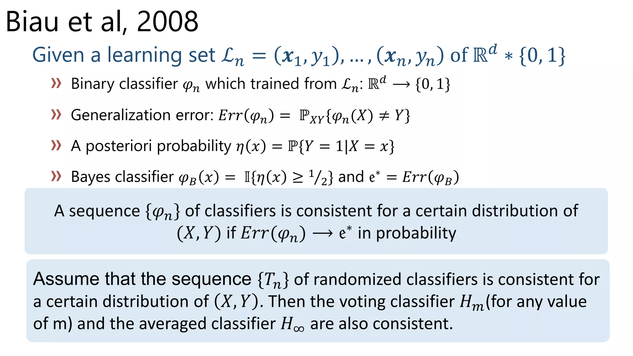
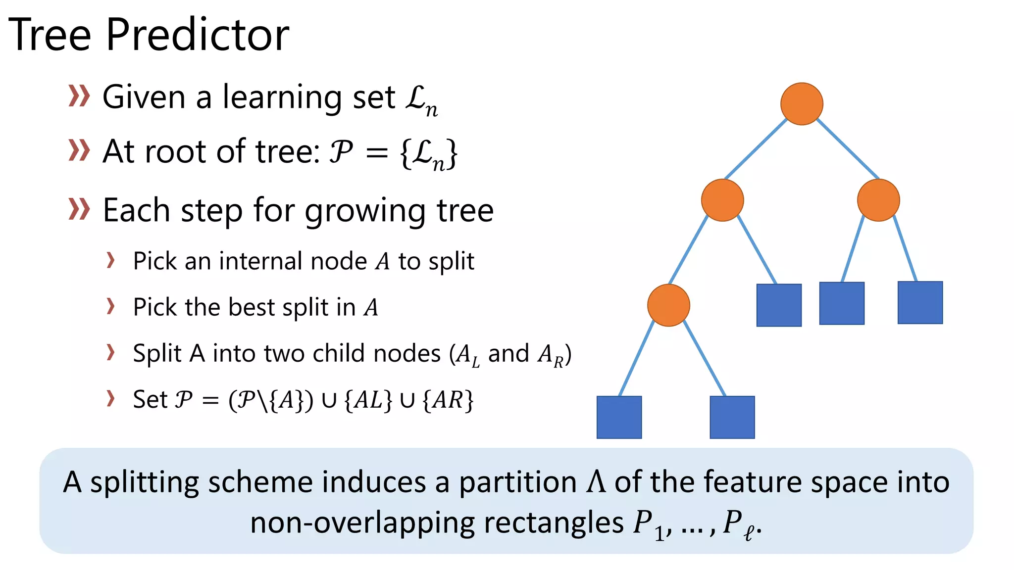
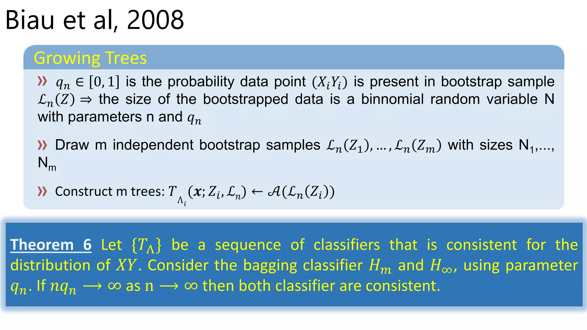
![Biau et al, 2008
Growing Trees
Node 𝐴 is randomly selected
The split feature j is selected uniformly at random from [1, … , 𝑝]
Finally, the selected node is split along the randomly chosen feature at a random location
* Recursive node splits do not depend on the labels 𝑦1, … , 𝑦𝑛
Theorem 2 Assume that the distribution of 𝑋 is supported on [0, 1] 𝑑
.
Then purely random forest classifier 𝐻∞ is consistent whenever 𝑘 ⟶
∞ and 𝑘
𝑛 ⟶ 0 as n ⟶ ∞.](https://image.slidesharecdn.com/talk4-151222141843/75/Conistency-of-random-forests-63-2048.jpg)
![Biau et al, 2012
Growing Trees
At each node, a coordinate is selected with 𝑝 𝑛𝑗 ∈ (0, 1) is the probability j-th feature is selected
the split is at the midpoint of the chosen side
Theorem 1 Assume that the distribution of 𝑋 has support on [0, 1] 𝑑
.
Then the random forests estimate 𝐻∞(𝒙; ℒ 𝑛) is consistent whenever
𝑝 𝑛𝑗 𝑙𝑜𝑔𝑘 𝑛 ⟶ ∞ for all j=1, …, p and 𝑘 𝑛
𝑛 ⟶ 0 as 𝑛 ⟶ ∞.](https://image.slidesharecdn.com/talk4-151222141843/75/Conistency-of-random-forests-65-2048.jpg)
![Biau et al, 2012
Assume that X is uniformly distributed on [0,1] 𝑝
𝒑 𝒏𝒋 = (𝟏/𝑺)(𝟏 + 𝝃 𝒏𝒋) 𝒇𝒐𝒓 𝒋 ∈ 𝓢
In sparse settings
Estimation Error (variance)
𝔼{[𝐻∞ 𝒙; ℒ 𝑛 − 𝐻∞ 𝒙; ℒ 𝑛 ]2} ≤ 𝐶𝜎2
S2
S − 1
𝑆
2𝑝
(1 + 𝜉 𝑛)
𝑘 𝑛
𝑛(𝑙𝑜𝑔𝑘 𝑛) 𝑆/2𝑝
If 𝑎 < 𝑝 𝑛𝑗 < 𝑏 form some constants 𝑎, 𝑏 ∈ 0,1 then
1 + 𝜉 𝑛 ≤
𝑆 − 1
𝑆2 𝑎 1 − 𝑏
𝑆
2𝑝](https://image.slidesharecdn.com/talk4-151222141843/75/Conistency-of-random-forests-66-2048.jpg)
![Biau et al, 2012
Assume that X is uniformly distributed on [0,1] 𝑝 and 𝜑 𝐵 𝒙 𝒮 is 𝐿 − 𝐿𝑖𝑝𝑠𝑐ℎ𝑖𝑡𝑧 on [0,1] 𝑠
𝒑 𝒏𝒋 = (𝟏/𝑺)(𝟏 + 𝝃 𝒏𝒋) 𝒇𝒐𝒓 𝒋 ∈ 𝓢
In sparse settings
Approximation Error (bias2)
𝔼 𝐻∞ 𝒙; ℒ 𝑛 − 𝜑 𝐵 𝒙
2
≤ 2𝑆𝐿2 𝑘 𝑛
−
0.75
𝑆𝑙𝑜𝑔2 1+𝛾 𝑛
+ [ sup
𝑥∈[0,1] 𝑝
𝜑 𝐵
2
(𝒙)]𝑒−𝑛/2𝑘 𝑛
where 𝛾 𝑛 = min
𝑗∈ 𝒮
𝜉 𝑛𝑗 tends to 0 as n tends to infinity.](https://image.slidesharecdn.com/talk4-151222141843/75/Conistency-of-random-forests-67-2048.jpg)
![Finite and infinite RFs [Scornet, 2014]
ℒ 𝑛 Θ𝑖 ℒ 𝑛
𝐻∞(𝒙; ℒ 𝑛) = 𝔼Θ{ Θ ℒ 𝑛 }
ℒ 𝑛
ℒ 𝑛 𝐻∞(𝒙; ℒ 𝑛)
Theorem 3.1 Conditionally on ℒ 𝑛, almost surely, for all 𝑥 ∈ 0, 1 𝑝
, we
have: 𝐻 𝑚 𝒙; ℒ 𝑛
𝑀→∞
𝐻∞(𝒙; ℒ 𝑛).](https://image.slidesharecdn.com/talk4-151222141843/75/Conistency-of-random-forests-68-2048.jpg)
![Finite and infinite RFs [Scornet, 2014]
One has 𝑌 = 𝑚 𝑋 + 𝜀 where 𝜀 is a centered Gaussian noise with
finite variance 𝜎2
, independent of 𝑋,
and 𝑚 ∞ = sup
𝑥∈[0,1] 𝑝
|𝑚(𝑥)| < ∞.
Assumption H
Theorem 3.3 Assume H is satisfied. Then, for all m, 𝑛 ∈ ℕ∗
,
𝐸𝑟𝑟 𝐻 𝑚 𝒙; ℒ 𝑛 = 𝐸𝑟𝑟 𝐻∞(𝒙; ℒ 𝑛) +
1
𝑚
𝔼 𝑋,ℒ 𝑛
[𝕍Θ[ 𝑇Λ (𝒙; Θ, ℒ 𝑛)]]
⇒ 𝑚 ≥
8 𝑚 ∞
2
+ 𝜎2
𝜀
+
32𝜎2
𝑙𝑜𝑔𝑛
𝜀
𝑡ℎ𝑒𝑛 𝐸𝑟𝑟 Hm − 𝐸𝑟𝑟 H∞ ≤ 𝜀
0 ≤ 𝐸𝑟𝑟 Hm − 𝐸𝑟𝑟 H∞ ≤
8
m
( 𝑚 ∞
2 + 𝜎2(1 + 4𝑙𝑜𝑔𝑛))](https://image.slidesharecdn.com/talk4-151222141843/75/Conistency-of-random-forests-69-2048.jpg)
![RF and Additive regression model [Scornet et al., 2015]
Growing Trees
without replacement
Assume that 𝐴 is selected node and 𝐴 > 1
Select uniformly, without replacement, a subset ℳ𝑡𝑟𝑦 ⊂ 1, … , 𝑝 , |ℳ𝑡𝑟𝑦| = 𝑚 𝑡𝑟𝑦
Select the best split in A by optimizing the CART-split criterion along the coordinates in ℳ𝑡𝑟𝑦
Cut the cell 𝐴 according to the best split. Call 𝐴 𝐿 and 𝐴 𝑅 the true resulting cell
Set 𝐴 𝐴 𝐿 𝐴 𝑅](https://image.slidesharecdn.com/talk4-151222141843/75/Conistency-of-random-forests-70-2048.jpg)
![RF and Additive regression model [Scornet et al., 2015]
𝑌 = 𝑗=1
𝑝
𝑚𝑗(𝑋(𝑗)
) + 𝜀
Assumption H1
Theorem 3.1 Assume that (H1) is satisfied. Then, provided 𝑛 ⟶ ∞ and
𝑡 𝑛(𝑙𝑜𝑔𝑎 𝑛)9
/𝑎 𝑛 ⟶ 0, is consistent.
Theorem 3.2 Assume that (H1) and (H2) are satisfied and let 𝑡 𝑛 = 𝑎 𝑛.
Then, provided 𝑎 𝑛 ⟶ ∞, 𝑡 𝑛 ⟶ ∞ and 𝑎 𝑛 𝑙𝑜𝑔𝑛/𝑛 ⟶ 0, is consistent.](https://image.slidesharecdn.com/talk4-151222141843/75/Conistency-of-random-forests-71-2048.jpg)
![RF and Additive regression model [Scornet et al., 2015]
, 𝑗1,𝑛 𝑋 , … , 𝑗 𝑘,𝑛 𝑋 the first cut directions used to construct
the cell containing 𝑋. 𝑗 𝑞,𝑛 𝑋 = ∞ if the cell has been cut strictly less than
q times.
Theorem 3.2 Assume that (H1) is satisfied. let k ∈ ℕ∗
and 𝜉 > 0.
Assume that there is no interval [𝑎, 𝑏] and no 𝑗 ∈ {1, … , 𝑆} such that
𝑚𝑗 is constant on [𝑎, 𝑏]. Then, with probability 1 − 𝜉, for all 𝑛 large
enough, we have, for all 1 ≤ 𝑞 ≤ 𝑘, 𝑗 𝑞,𝑛 𝑋 ∈ {1, … , 𝑆}.](https://image.slidesharecdn.com/talk4-151222141843/75/Conistency-of-random-forests-72-2048.jpg)
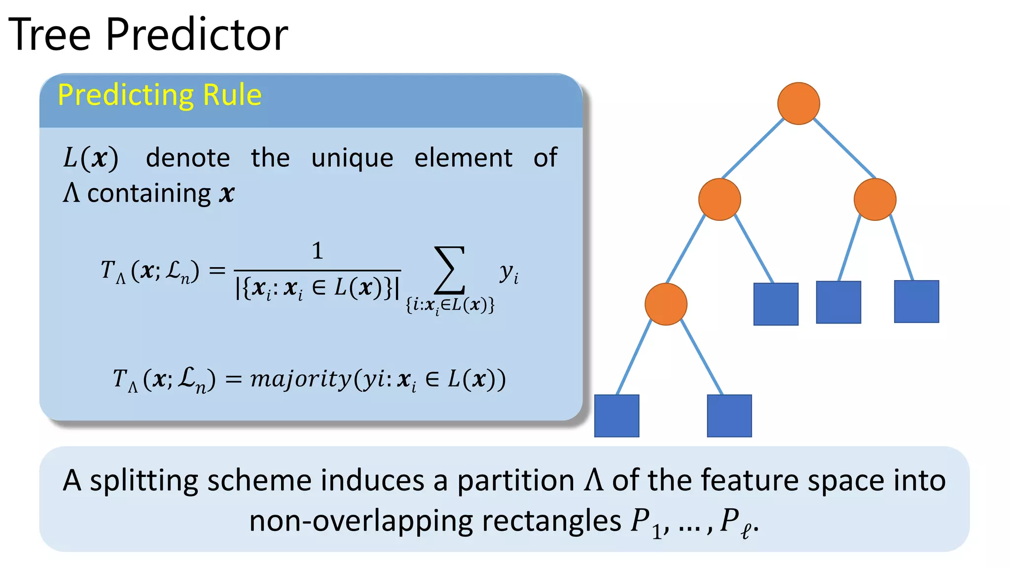
![[Wager, 2015]
A partition Λ is 𝛼, 𝑘 − 𝑣𝑎𝑙𝑖𝑑 if can generated by a recursive partitioning scheme in
which each child node contains at least a fraction 𝛼 of the data points in its parent
node for some 0 < 𝛼 < 0.5, and each terminal node contains at least 𝑘 training
examples for some k ∈ N.
Given a dataset 𝑋, 𝒱𝛼,𝑘(𝑋) denote the set of 𝛼, 𝑘 − 𝑣𝑎𝑙𝑖𝑑 partitions
𝑇Λ: [0,1] 𝑝→ ℝ, 𝑇Λ 𝒙 =
1
|{𝒙 𝑖: 𝒙 𝑖 ∈ 𝐿(𝒙)}| {𝑖: 𝒙 𝑖∈𝐿(𝒙)} 𝑦𝑖 (is called valid tree)
𝑇Λ
∗
: [0,1] 𝑝→ ℝ, 𝑇Λ
∗
𝒙 = 𝔼[𝑌|𝑋 ∈ 𝐿(𝒙)] (is called partition-optimal tree)
Whether we can treat 𝑇Λ as a good approximation to 𝑇Λ
∗
the
supported on the partition Λ](https://image.slidesharecdn.com/talk4-151222141843/75/Conistency-of-random-forests-73-2048.jpg)
![Given a learning set ℒ 𝑛 of [0,1] 𝑝
∗ −
𝑀
2
,
𝑀
2
with 𝑋~𝑈([0,1] 𝑝
)
[Wager, 2015]
Theorem 1
Given parameters n, p, k such that
lim
𝑛→∞
log 𝑛 log 𝑝
𝑘
= 0 𝑎𝑛𝑑 𝑝 = Ω(𝑛)
then
lim
𝑛,𝑑,𝑘→∞
ℙ sup
𝑥∈ 0,1 𝑝,Λ∈𝒱 𝛼,𝑘
|𝑇Λ − 𝑇Λ
∗
| ≤ 6𝑀
log 𝑛 log(𝑝)
klog((1 − 𝛼)−1)
= 1](https://image.slidesharecdn.com/talk4-151222141843/75/Conistency-of-random-forests-74-2048.jpg)
![[Wager, 2015]
Growing Trees (Guest-and-check)
Select a currently un-split node 𝐴 containing at least 2k training examples
Pick a candidate splitting variable 𝑗 ∈ {1, … , 𝑝} uniformly at random
Pick the minimum squared error (ℓ( 𝜃)) splitting point 𝜃
If either there has already been a successful split along variable j for some other nod or
ℓ( 𝜃) ≥ 36𝑀2
log 𝑛 log(𝑑)
𝑘𝑙𝑜𝑔((1 − 𝛼)−1)
The split succeeds and we cut the node 𝐴 at 𝜃 along the j-th variable; if not we do not split the
node 𝐴 this time.](https://image.slidesharecdn.com/talk4-151222141843/75/Conistency-of-random-forests-75-2048.jpg)
![[Wager, 2015]
In sparse settings
and a set of sign variables 𝜎𝑗 ∈ ±1 such that, for all
𝑗 ∈ and all 𝑥 ∈ [0,1] 𝑝,
𝔼 𝑌 𝑋 −𝑗
= 𝑥 −𝑗
, 𝑋 𝑗
>
1
2
− 𝔼 𝑌 𝑋 −𝑗
= 𝑥 −𝑗
, 𝑋 𝑗
≤
1
2
≥ 𝛽𝜎𝑗
Assumption H1
is Lipschitz-continuous in
Assumption H2](https://image.slidesharecdn.com/talk4-151222141843/75/Conistency-of-random-forests-76-2048.jpg)
![[Wager, 2015]
In sparse settings
and a set of sign variables 𝜎𝑗 ∈ ±1 such that, for all
𝑗 ∈ and all 𝑥 ∈ [0,1] 𝑝,
𝔼 𝑌 𝑋 −𝑗
= 𝑥 −𝑗
, 𝑋 𝑗
>
1
2
− 𝔼 𝑌 𝑋 −𝑗
= 𝑥 −𝑗
, 𝑋 𝑗
≤
1
2
≥ 𝛽𝜎𝑗
Assumption H1
is Lipschitz-continuous in
Assumption H2
Theorem 2 Under the conditions of theorem 1, suppose that
assumptions in the sparse setting hold, then guest-and-check forest is
consistent.](https://image.slidesharecdn.com/talk4-151222141843/75/Conistency-of-random-forests-77-2048.jpg)
![[Wager, 2015]
𝐻{Λ}1
𝐵: [0,1] 𝑝→ ℝ, 𝐻 Λ 1
𝐵 𝒙 =
1
𝐵 𝑏=1
𝐵
𝑇Λ 𝑏
(𝒙) (is called valid forest)
𝐻{Λ}1
𝐵
∗
: [0,1] 𝑝→ ℝ, 𝐻{Λ}1
𝐵
∗
𝒙 =
1
𝐵 𝑏=1
𝐵
𝑇Λ 𝑏
∗
(𝒙) (is called partition-optimal forest)
Theorem 4
lim
𝑛,𝑑,𝑘→∞
ℙ sup
𝐻∈ℋ 𝛼,𝑘
1
𝑛
𝑖=1
𝑛
(𝑦𝑖 − 𝐻(𝑥𝑖))2 − 𝔼[(𝑌 − 𝐻(𝑋))2] ≤ 11𝑀2
log 𝑛 log(𝑝)
klog((1 − 𝛼)−1)
= 1](https://image.slidesharecdn.com/talk4-151222141843/75/Conistency-of-random-forests-78-2048.jpg)
![RF and Additive regression model [Scornet et al., 2015]
the indicator that falls in the same cell as in the
random tree designed with ℒn and the random parameter
where ′is an independent copy of .
′, 𝑋1, … , 𝑋 𝑛,
′
, 𝑋1, … , 𝑋 𝑛](https://image.slidesharecdn.com/talk4-151222141843/75/Conistency-of-random-forests-82-2048.jpg)
![RF and Additive regression model [Scornet et al., 2015]](https://image.slidesharecdn.com/talk4-151222141843/75/Conistency-of-random-forests-83-2048.jpg)

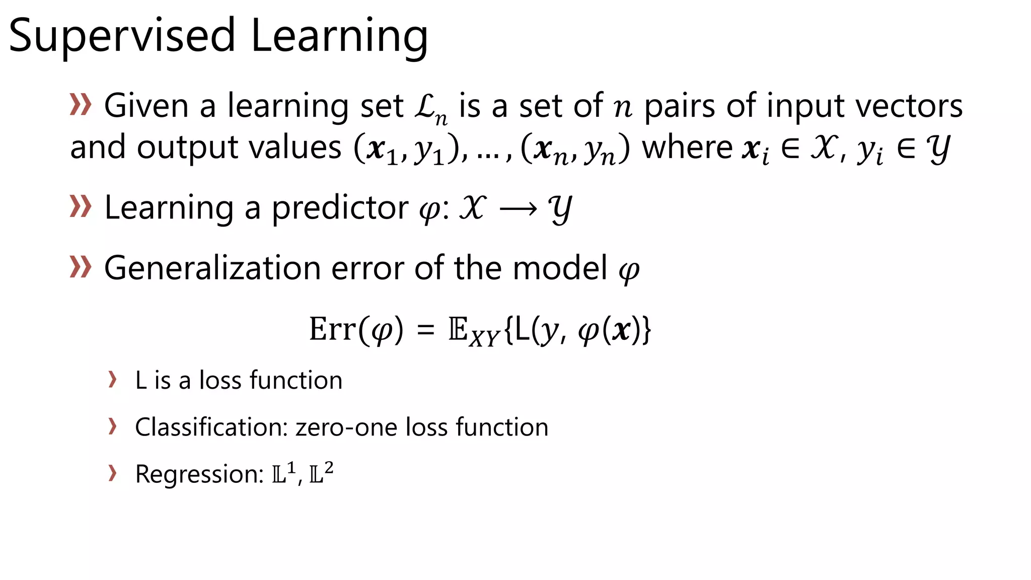
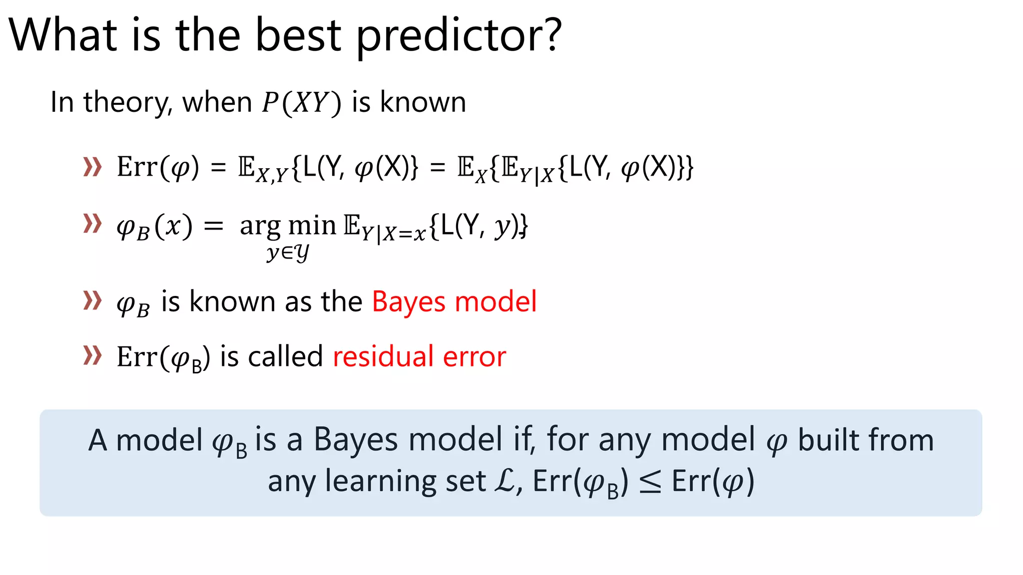
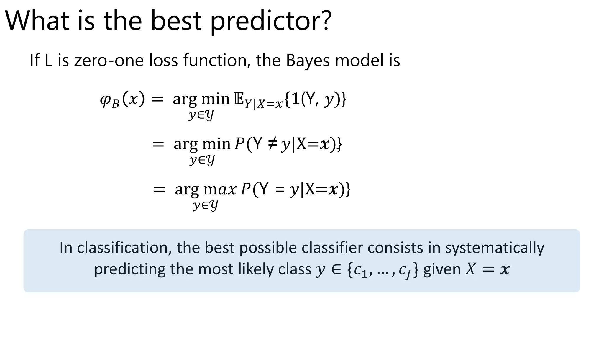
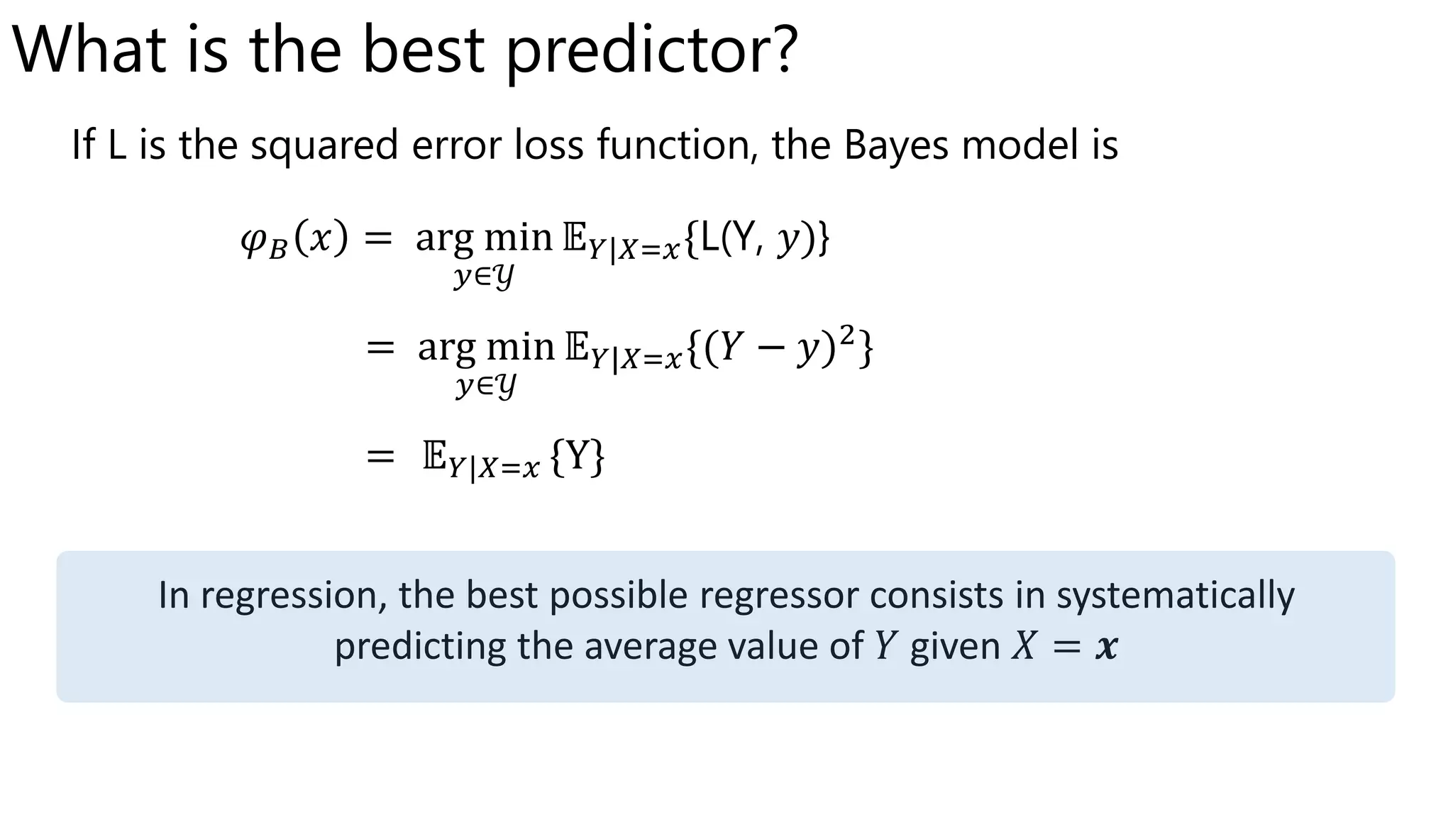
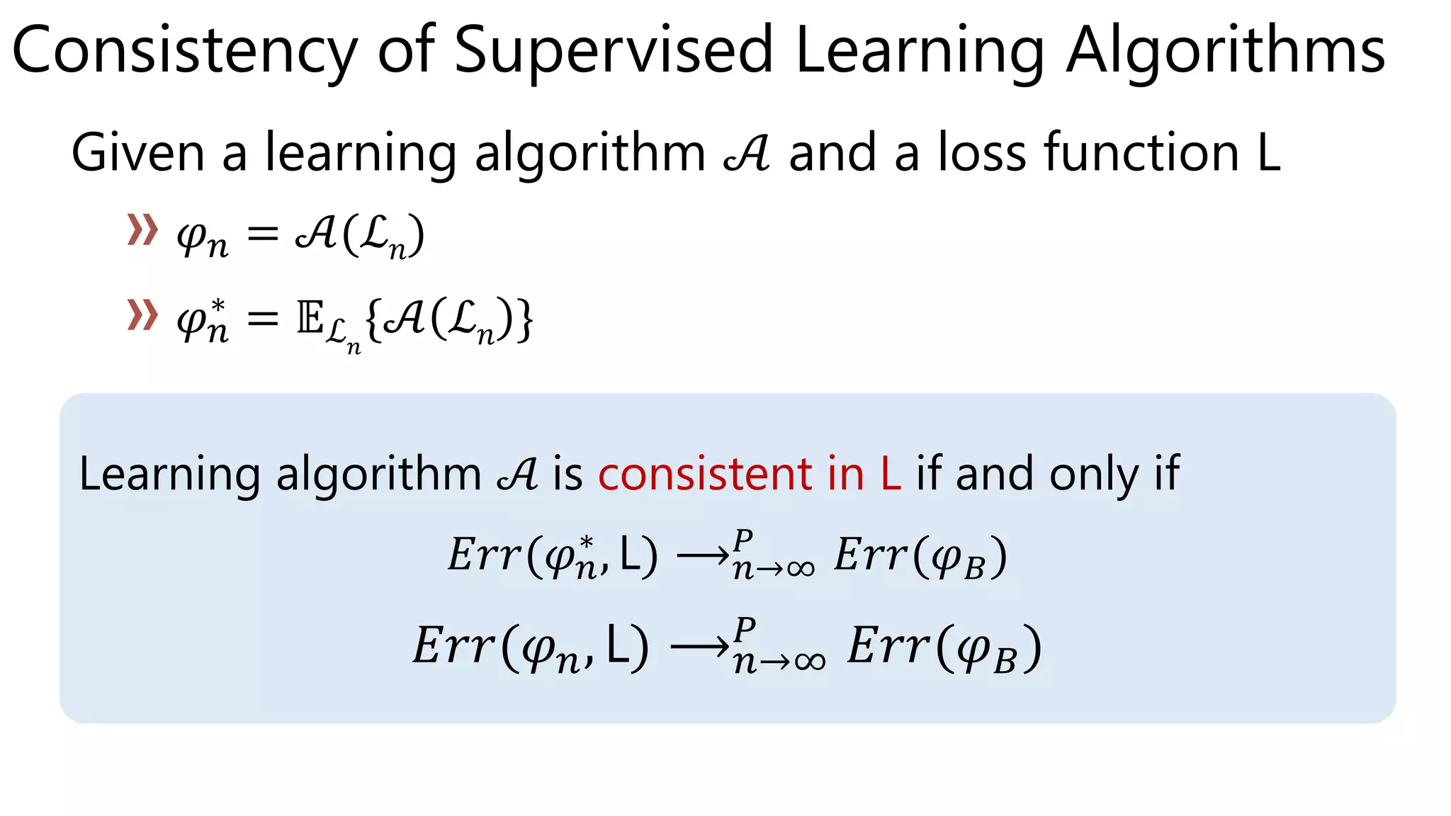
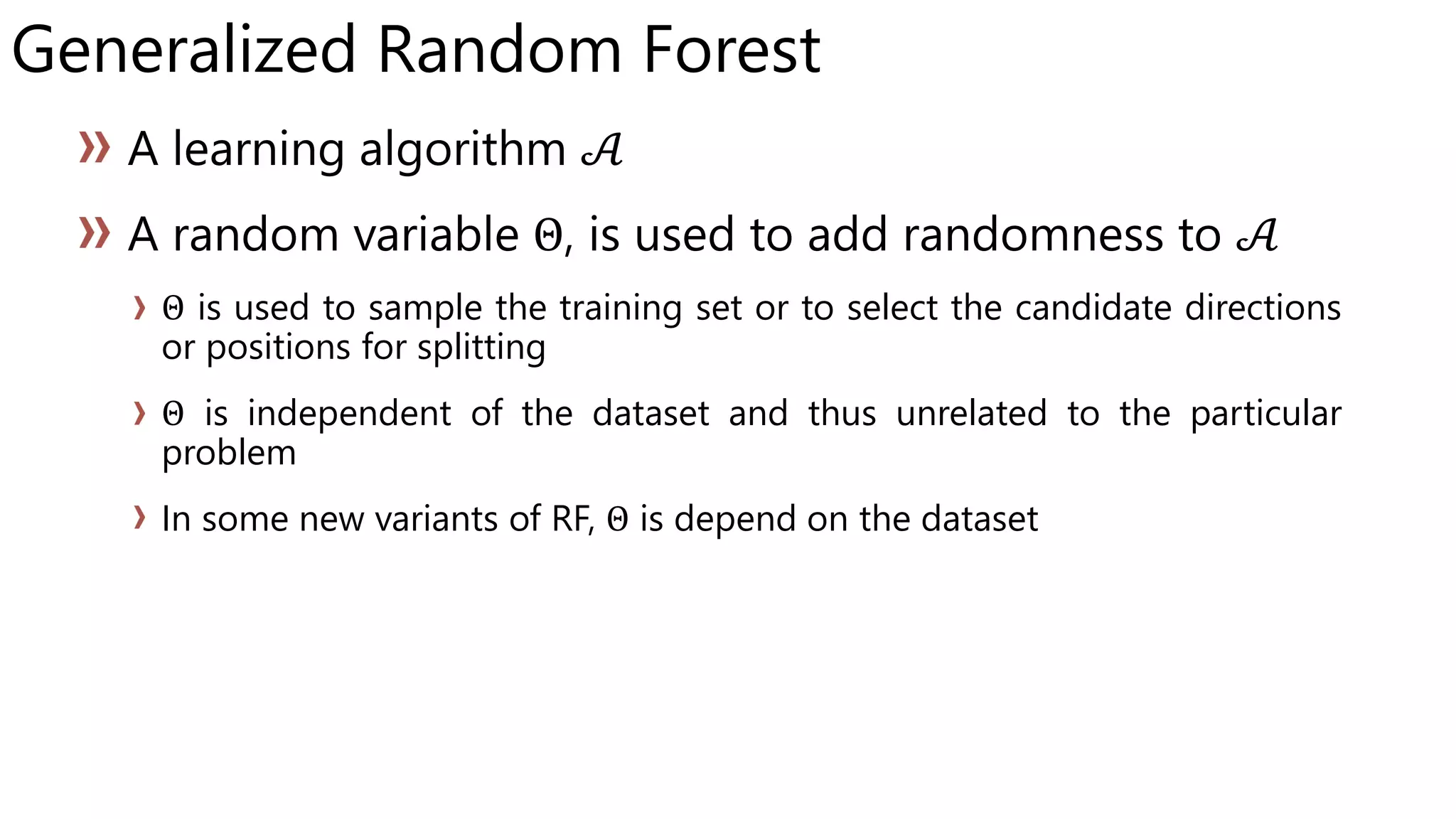
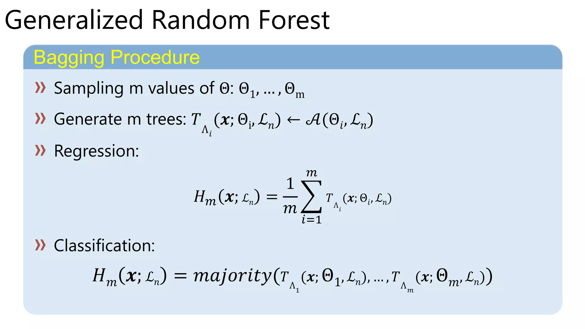
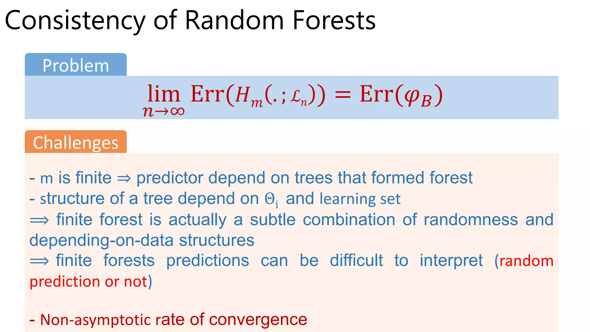
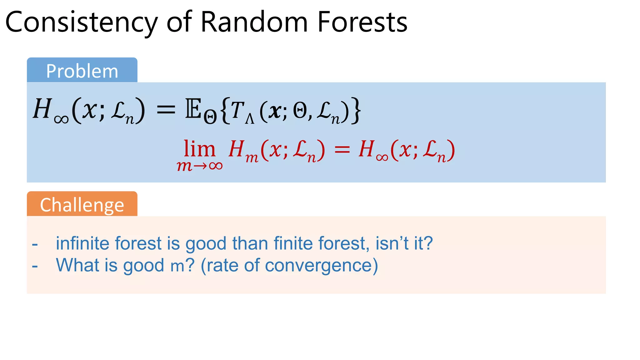
The document discusses consistency of random forests. It summarizes recent theoretical results showing that random forests are consistent estimators under certain conditions. Specifically, it is shown that random forests are consistent if the number of features sampled at each node (mtry) increases with sample size and the minimum node size decreases with sample size. The document also discusses how consistency holds even when the splitting criteria are randomized, as in random forests, as long as the base classifiers are consistent.


![Vibe Coding vs. Spec-Driven Development [Free Meetup]](https://cdn.slidesharecdn.com/ss_thumbnails/vibecodingvsspecdrivendevelopment-251209105622-43f455e7-thumbnail.jpg?width=640&height=640&fit=bounds)


