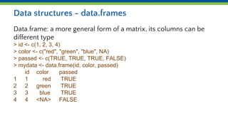
R provides several data structures for storing and manipulating data, including matrices, data frames, and lists. Matrices store data of the same type arranged in rows and columns, while data frames allow columns to contain different data types. Lists are flexible containers that can hold different data types and named components. These structures enable accessing and subsetting elements using row/column names or indices, and performing element-wise operations on the data.

1. R structures & objects: matrices and
data frames
Day 1 - Introduction to R for Life Sciences

2. Matrices
A matrix is a “vector in the shape of a table”
All items in the matrix are the same data type
Can be built from rows using rbind(), or from columns using cbind(),
or using matrix()
> rbind( 1:3, 11:13)
[,1] [,2] [,3]
[1,] 1 2 3
[2,] 11 12 13
> cbind(11:13, 23:25)
[,1] [,2]
[1,] 11 23
[2,] 12 24
[3,] 13 25

3. Using the matrix function
> x <- matrix(1:6, nrow=2, byrow=TRUE)
[,1] [,2] [,3]
[1,] 1 2 3
[2,] 4 5 6
Row and column names make life easier!
> x <- matrix(1:6, nrow=2, byrow=TRUE,
dimnames=list( c(“geneA”, “geneB”), c(“delA”, “delB”, “delC”))
delA delB delC
geneA 1 2 3
geneB 4 5 6

4. Data structures - data.frames
Data.frame: a more general form of a matrix, its columns can be
different type
> id <- c(1, 2, 3, 4)
> color <- c("red", "green", "blue", NA)
> passed <- c(TRUE, TRUE, TRUE, FALSE)
> mydata <- data.frame(id, color, passed)
id color passed
1 1 red TRUE
2 2 green TRUE
3 3 blue TRUE
4 4 <NA> FALSE

5. Operations are always element-wise
> a <- 1:3
> b <- 4:6
> a + b
5 7 9
> b^a # ‘raised to power’
4 25 216
> p <- matrix(1:4, ncol=2,
byrow=TRUE)
> q <- cbind(c(10, 10), c(100,100))
> p*q
[,1] [,2]
[1,] 10 200
[2,] 30 400

6. Useful functions
str() # display the data structure
summary() # display a summary of the data
length() # get the length of a vector or list (data.frame: nrow!)
dim() # get the dimensions of a data.frame or matrix
head() # show the first part of a data structure
You can also explore your data in the Environment window!

7. Dimensions of data.frames and matrices
> x <- matrix(1:6, nrow=2, byrow=TRUE)
[,1] [,2] [,3]
[1,] 1 2 3
[2,] 4 5 6
x[ i, j ]
index before the comma: indicates the row(s). If missing: all rows
index after the comma: indicates column(s). If missing: all columns

8. Example
> x
[,1] [,2] [,3]
[1,] 1 2 3
[2,] 4 5 6
Using integers:
> x[2, 3] # the value on the second row, third column
> x[ , 2] # all rows, second column. So: the whole 2nd column
> x[ , c(1,3)] # the first and third column (new data.frame or matrix!)
> x[ , -2] # everything but the second column
> x[ , 1:3] # first up to and including third column

9. Data Frames
data.frames
> mydata[ , "id"]
> mydata$id # does the same thing

10. Using logicals:
delA delB delC
geneA 1 2 3
geneB 4 5 6
> ind <- c(FALSE, TRUE, TRUE)
> x[ 1 , ind] # first row; first column:no, 2nd, 3rd column: yes
[1] 2 3

11. Using characters:
> x <- matrix(1:6, nrow=2, byrow=TRUE,
dimnames=list( c("geneA", "geneB"), c("delA", "delB", "delC"))
delA delB delC
geneA 1 2 3
geneB 4 5 6
> x["geneB", "delA"] # selects the value of geneB in delA
> x[, c("delA", "delC")] # selects columns delA and delC

12. Logical vector and selection
Often (implicitly) used in combination with select statements
delA delB delC
geneA 1 2 3
geneB 4 5 6
> ind <- x["geneA", ] > 1
[1] FALSE TRUE TRUE
> x["geneA", ind]
[1] 2 3

13. Operators
delA delB delC
geneA 1 2 3
geneB 4 5 6
> ind <- x["geneA", ] > 1 & x["geneA", ] < 3
> x["geneA", ind]
[1] 2

14. Data structures - lists
An ordered collection of "things"
> a <- c(1, 2, 3, 4)
> mylist <- list(name="Patrick", numbers=a, age=38)
$name
[1] "Patrick"
$numbers
[1] 1 2 3 4
$age
[1] 38

15. Specifics for lists
lists
>mylist <- list(analysis=”GSEA”, genes=c(“Foxo3a”, “TP53”), cutoff=0.05)
> mylist$analysis
> mylist$genes[2]

16. Data types - factors
Factors deal with categorical variables
> gender <- factor(c(rep("male", 2), rep("female", 3)))
> gender
[1] male male female female female the actual values
Levels: female male allowed values
> str(gender)
Factor w/ 2 levels "female","male": 2 2 1 1 1

17. Ordering
(Re)order a data.frame or matrix using the values from a single
column using order()
> mydata <- data.frame( id=c(1,3,4,2), name=c("geneB", "geneA", "geneD",
"geneC"), value=c(-0.2, 1.5, -3, 3))
> mydata[order(mydata[, "id"]), ] # sort on id
> mydata[order(mydata[, "name"]), ] # sort on name