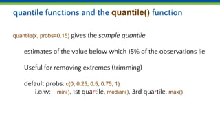
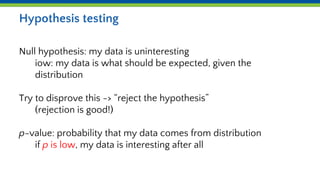
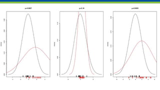
This document introduces various statistical functions in R including descriptive statistics like mean, median, and standard deviation. It covers distribution functions like the normal distribution and functions for generating random values. Hypothesis tests like the t-test are discussed along with ANOVA and linear models. Quantile functions and plotting are also introduced for understanding data distributions and removing outliers.

1. Statistical functions
Day 5 - Introduction to R for Life Sciences

2. Statistical functions
Descriptive statistics:
min(), max(), mean(), median(), sd(), var(), mad(), IQR(),
quantile() and cor(), cov()
Distribution functions
Hypothesis tests:
t.test(), wilcox.test(), var.test(), shapiro.test(), ks.test(), cor.test()
anova/linear models

3. What are distributions?
The (idealized) shape of your reference data
expression values, binding data, cell counts, read depth, ....
Why do we need them?
E.g. to calculate how probable an observed deviation is
→ p-values
R knows many different distributions
E.g. Normal, Uniform, Poisson, etc. etc. ….

4. Distribution functions in R (shown for Normal)
dnorm density function (shows shape of distribution)
pnorm cum. distribution function (needed for p-vals)
qnorm quantile function (inverse of distribution function)
rnorm generates values that belong to the normal
distribution
set.seed(3498) Reset the random number generator

6. Randomization of existing values
> sample(1:10)
[1] 8 3 5 7 4 9 6 1 10 2
> sample(1:10, size=4)
[1] 1 9 7 6
> sample(c(TRUE, FALSE), 6, replace=TRUE)
[1] FALSE TRUE FALSE TRUE FALSE FALSE
> sample(c("A", "C", "G", "T"), 16, replace=TRUE)
[1] "T" "T" "A" "T" "C" "C" "A" "G" "A" "G" "C" "A" "A" "T" "G" "C"

7. quantile functions and the quantile() function
quantile(x, probs=0.15) gives the sample quantile
estimates of the value below which 15% of the observations lie
Useful for removing extremes (trimming)
default probs: c(0, 0.25, 0.5, 0.75, 1)
i.o.w: min(), 1st quartile, median(), 3rd quartile, max()

8. Trimming
> quantile(x, probs=c(0.05, 0.95))
5% 95%
-1.404072 1.879870
> limits <- quantile(x, probs=c(0.05, 0.95))
> x <- x [ x > limits[1] & x < limits[2] ]
← these are just the names ...

9. Quantile plots
Check whether your observations conform to a particular
distribution
qqnorm()
Compares to the Normal distribution
qqplot()
Compares to other distributions
Line should be straight

10. Quantile plot example

11. Correlation
Number between -1 and 1; -1 and 1 strong similarity; 0 no similarity
Calculate with cor(x, y)

12. Hypothesis testing
Null hypothesis: my data is uninteresting
iow: my data is what should be expected, given the
distribution
Try to disprove this -> “reject the hypothesis”
(rejection is good!)
p-value: probability that my data comes from distribution
if p is low, my data is interesting after all

13. tests in R
Look like X.test(a.values, b.values)
e.g. t.test()
t-test gives the significance (p-value) for the difference in the
averages of two samples.

15. tests return a list(), but print something else
t.test(x,y) →
Welch Two Sample t-test
data: x and y
t = -2.8096, df = 15.245, p-value = 0.01304
alternative hypothesis: true difference in means
is not equal to 0
95 percent confidence interval:
-2.0611160 -0.2843106
sample estimates:
mean of x mean of y
-0.08099273 1.09172057
> str(t)
List of 9
$ statistic : Named num -2.81
$ parameter : Named num 15.2
$ p.value : num 0.013
$ conf.int : atomic [1:2] -2.061 -0.284
$ estimate : Named num [1:2] -0.081 1.092
$ null.value : Named num 0
$ alternative: chr "two.sided"
$ method : chr "Welch Two Sample t-test"
$ data.name : chr "x and y"