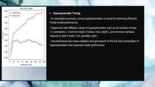
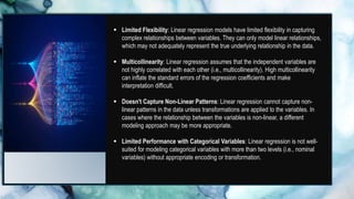
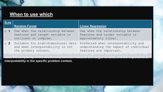
SlideShare a Scribd company logo
1 of 97
A Presentation on Random Forest
and Linear Regression
Created by:-
Shouvic Banik
Machine Learning and Decision Tree
What is Machine Learning?
 Machine learning is a subset of artificial intelligence (AI) that focuses on the
development of algorithms that enable computers to learn and improve from
experience without being explicitly programmed.
 It involves the use of statistical techniques to enable computers to learn patterns
from data and make predictions or decisions.
Importance of Machine Learning in Various Fields
Machine learning has revolutionized numerous industries by providing solutions to
complex problems and making processes more efficient.
Applications of machine learning span various fields including:
 Healthcare: Diagnosis, personalized treatment, drug discovery.
 Finance: Fraud detection, risk assessment, algorithmic trading.
 Marketing: Customer segmentation, recommendation systems, sentiment analysis.
 Transportation: Autonomous vehicles, route optimization, predictive maintenance.
 Retail: Demand forecasting, inventory management, customer behavior analysis.
Decision Tree in Machine Learning
 Flowchart-like tree structure with internal nodes representing features, branches
representing rules, and leaf nodes representing algorithm results.
 Versatile supervised machine-learning algorithm used for classification and
regression.
 Powerful algorithm used in Random Forest for training on different training data
subsets.
Tree structure
A decision tree is a flowchart-like structure in which each internal node represents a
test on an attribute, each branch represents the outcome of the test, and each leaf
node represents a class label.
Advantages and Disadvantages of decision tree
Advantages:
 Compared to other algorithms, decision trees require less data preparation during
pre-processing.
 A decision tree does not require normalization of data.
 A decision tree does not require scaling of data as well.
Disadvantages:
 A small change in the data can cause a large change in the decision tree structure
causing instability.
 For a Decision tree sometimes, the calculation can go far more complex than other
algorithms.
 Decision tree often involves higher time to train the model.
Random Forest Algorithm
Description of Random Forest
 A "Random Forest" is a method used in machine learning to improve the accuracy
of decision trees.
 It works by creating multiple decision trees during training and then choosing the
most common class among them. This helps to prevent overfitting by randomly
selecting some features for each decision tree.
 It is a popular ensemble learning technique used for both classification and
regression tasks in machine learning.
Overview of Ensemble Learning:
 Ensemble learning combines multiple models to improve the performance of the
overall system.
 It leverages the "wisdom of the crowd" principle, where combining multiple weak
learners can produce a strong learner.
 Ensemble methods typically work by training multiple models independently and
then combining their predictions to produce a final output.
 Random Forest is one of the most powerful and widely used ensemble learning
techniques due to its simplicity, scalability, and robustness
Why Choose Random Forest?
The Need for Random Forest Algorithm
Random Forest is a popular choice in machine learning due to its ability to overcome challenges in
traditional algorithms.
Some of the key reasons for using Random Forest include:
 High Dimensionality: Random Forest works well with data that has many features compared to the
number of samples.
 Overfitting: Random Forest is less prone to overfitting compared to individual decision trees,
making it more robust and generalizable.
 Feature Importance: It provides a built-in feature importance measure, allowing users to
understand the relative importance of different features in the prediction process.
 Handling Missing Data: Random Forest is a type of algorithm that can handle missing data in a
useful way. This is done by filling in the missing information and still maintaining accurate
predictions.
 Non-linear Relationships: It can capture complex, non-linear relationships between features and
target variables, making it suitable for a wide range of data types.
Comparison with Other Machine Learning Algorithms
Random Forest offers several advantages over other machine-learning algorithms:
 Decision Trees: Random Forest overcomes the limitations of individual decision
trees by aggregating multiple trees, reducing the risk of overfitting and improving
predictive performance
 Support Vector Machines (SVM): While SVMs are powerful for small to medium-
sized datasets, Random Forest tends to perform better on large datasets due to its
parallelizable nature and efficient computation.
 Neural Networks: Random Forest often requires less data preprocessing and
tuning compared to neural networks, making it more accessible and easier to
implement for many practitioners. Additionally, it provides transparent models,
making it easier to interpret and explain predictions.
Functioning Random Forest
Random Forest as a Collection of Decision Trees
 Random Forest consists of a collection of decision trees, where each
tree is trained independently.
 During training, each tree is built using a random subset of the training
data (bootstrap samples) and a random subset of the features.
 The randomness introduced during the construction of individual trees
helps to decorrelate them, reducing the risk of overfitting and improving
the overall predictive performance.
 In classification tasks, the final prediction of Random Forest is
determined by a majority vote (mode) of the predictions of individual
trees. In regression tasks, it's determined by averaging the predictions of
individual trees.
 By combining the predictions of multiple trees, Random Forest provides
a robust and accurate model that is less sensitive to noise and outliers in
the data.
Algorithm
Functioning of the Algorithm
- Random Forest is an ensemble learning technique that combines the predictions of
multiple decision trees to improve predictive accuracy and reduce overfitting.
- The algorithm consists of three main steps:
 Random selection of bootstrap samples from the training data.
 Construction of decision trees using the bootstrap samples and a subset of
features.
 Aggregation of predictions from individual trees to make the final prediction.
Splitting Criteria
 At each node of the decision tree, Random Forest uses a splitting criterion to
partition the data into subsets based on the values of a selected feature.
 The most common splitting criteria include:
 Gini impurity: Measures the probability of misclassifying a randomly chosen
element if it were randomly labelled according to the distribution of labels in the
node.
 Information gain (Entropy): Measures the reduction in entropy or uncertainty about
the class labels after the split.
Bootstrapping
 Bootstrapping is a sampling technique where random samples are drawn with
replacements from the original dataset.
 In Random Forest, each decision tree is trained on a different bootstrap sample
created from the original dataset.
 Bootstrapping introduces randomness into the training process, which helps to
decorrelate the individual trees and reduce overfitting.

Aggregation
 After constructing multiple decision trees, Random Forest aggregates their
predictions to make the final prediction.
 In classification tasks, the final prediction is determined by a majority vote (mode)
of the predictions of individual trees.
 In regression tasks, the final prediction is determined by averaging the
predictions of individual trees.
 Aggregation helps to improve the robustness and accuracy of the model by
combining the predictions of multiple trees.
By leveraging bootstrapping, splitting criteria, and aggregation, Random Forest
creates an ensemble of diverse decision trees that collectively provide a powerful
and reliable predictive model.
Advantages
The advantages of the Random Forest algorithm are as
follows:
 Robustness to Overfitting:
- Random Forest is less prone to overfitting compared to individual decision trees.
- By combining multiple decision trees trained on different subsets of data, Random
Forest reduces the risk of capturing noise and outliers in the training data.
 Handling Missing Values:
- Random Forest can effectively handle missing values in the dataset.
- During the construction of individual trees, missing values are handled by using the
available features for splitting without imputation.
- This ability to handle missing data makes Random Forest robust to real-world
datasets with common missing values.
 Efficient on Large Datasets:
- Random Forest is well-suited for large datasets due to its parallelizable nature and
efficient computation.
- The training process can be easily parallelized across multiple CPU cores or
distributed computing clusters, making it scalable to large datasets.
- Additionally, Random Forest requires minimal data preprocessing compared to other
algorithms, resulting in faster model development and deployment.
 Feature Importance:
- Random Forest provides a built-in feature importance measure, allowing users to
understand the relative importance of different features in the prediction process.
- This feature is valuable for feature selection, model interpretation, and identifying the
most relevant features for prediction.
 Versatility:
- Random Forest can be applied to both classification and regression tasks.
- It can handle a variety of data types, including categorical and numerical features,
without the need for extensive feature engineering.
 High Accuracy:
- Random Forest often achieves high predictive accuracy compared to other machine
learning algorithms.
- By aggregating the predictions of multiple decision trees, Random Forest leverages
the collective wisdom of the ensemble to produce accurate and reliable predictions.
Applications
Some applications of the Random Forest algorithm are as follows:
 Application for Image Classification :
-
 Random Forest is used in image classification tasks to classify objects, scenes, or
patterns within images.
 It can be applied in various domains such as:
 Medical imaging: Identifying tumors, lesions, or abnormalities in medical images
like X-rays, MRIs, or CT scans.
 Satellite imagery: Analysing satellite images for land cover classification, urban
planning, and environmental monitoring.
 Autonomous vehicles: Detecting and recognizing objects on the road, such as
pedestrians, vehicles, and traffic signs.
Application for Fraud Detection:
Random Forest is utilized in fraud detection systems to identify fraudulent activities
or transactions.
 It can analyze large volumes of transaction data and detect anomalies or
patterns indicative of fraudulent behavior.
 Applications include:
 Banking and finance: Detecting credit card fraud, identity theft, money
laundering, and insider trading.
 Insurance: Identifying fraudulent insurance claims and suspicious activities
related to claims processing.
 E-commerce: Preventing fraudulent activities such as fake reviews, account
takeover, and payment fraud.
Application for Medical Diagnosis:
 Random Forest is employed in medical diagnosis to assist healthcare professionals
in diagnosing diseases and predicting patient outcomes.
 It can analyze patient data, including medical records, lab results, and diagnostic
images, to provide diagnostic support and treatment recommendations.
 Examples of medical diagnosis applications include:
 Disease diagnosis: Diagnosing diseases such as cancer, diabetes, heart disease,
and neurological disorders based on patient symptoms and medical tests.
 Risk assessment: Predicting the risk of developing certain diseases or
complications based on genetic factors, lifestyle choices, and medical history.
 Treatment response prediction: Estimating the likelihood of treatment success or
failure for specific therapies or medications based on patient characteristics and
biomarkers.
Implementation
Tools and Libraries for Implementing Random Forest
 Scikit-learn:
- Scikit-Learn is a popular machine-learning library in Python that provides a simple and efficient
implementation of the Random Forest algorithm.
- It includes the `RandomForestClassifier` for classification tasks and `RandomForestRegressor`
for regression tasks.
 R:
- Random Forest is also well-supported in the R programming language, and the `Random Forest`
package is widely used for implementing Random Forest models.
 H2O.ai:
- H2O.ai is an open-source software for data analysis that includes an implementation
of Random Forest.
- H2O's Random Forest implementation is distributed and scalable, making it suitable
for large datasets.
 Apache Spark MLlib:
- Apache Spark MLlib, a machine learning library for Apache Spark, provides a
distributed implementation of Random Forest.
- It is designed for big data processing, making it suitable for working with large
datasets
Parameters Tuning
 Hyperparameters in Random Forest:
- Random Forest has several hyperparameters that can be tuned to optimize the
model's performance.
- Some key hyperparameters include the number of trees (`n_estimators`), the
maximum depth of the trees (`max_depth`), the minimum number of samples required
to split a node (`min_samples_split`), and the maximum number of features considered
for splitting (`max_features`).
 Importance of Tuning Parameters:
- Tuning hyperparameters is crucial for optimizing the performance of a Random
Forest model.
- Proper tuning helps prevent overfitting(an undesirable machine learning behavior that
occurs when the machine learning model gives accurate predictions for training data
but not for new data) by controlling the complexity of the model and improving its
generalization ability.
- By adjusting hyperparameters, we can find the best combination that maximizes the
model's predictive accuracy on unseen data.
 Cross-Validation:
- Cross-validation is a technique used to evaluate the performance of a model and
tune hyperparameters.
- In k-fold cross-validation, the training dataset is divided into k subsets (folds), and
the model is trained and evaluated k times, each time using a different fold as the
validation set.
- Average performance across all k folds is the final metric.
- Cross-validation helps ensure the model's performance estimate is reliable and
reduces the risk of overfitting the training data.
Performance Improvement
Methods to Improve Random Forest Model
Performance
 Feature Engineering:
- Feature engineering involves creating new features or transforming existing
ones to improve the performance of machine learning models.
- In Random Forest, feature engineering can include:
- Creating interaction features by combining existing features.
- Transforming numerical features to make their distribution more Gaussian-
like.
- Encoding categorical variables using techniques like one-hot encoding or
ordinal encoding.
- Extracting relevant information from text or image data using feature
extraction techniques.
 Feature Selection:
- Feature selection aims to identify the most relevant features that contribute the
most to the predictive performance of the model.
- Random Forest provides built-in feature importance scores that can be used for
feature selection.
- Techniques for feature selection include:
- Selecting top features based on feature importance scores.
- Using recursive feature elimination (RFE) to iteratively remove the least
important features.
- Applying domain knowledge to select features that are most relevant to the task
at hand.
 Hyperparameter Tuning:
- As described previously, tuning hyperparameters is crucial for optimizing Random
Forest model performance.
- Experiment with different values of hyperparameters such as the number of trees
(`n_estimators`), maximum depth of trees (`max_depth`), and minimum samples
required to split a node (`min_samples_split`).
- Use techniques like cross-validation and grid search to find the best combination of
hyperparameters that maximize model performance.
 Handling Imbalanced Data:
- If the dataset is imbalanced, where one class is significantly more prevalent
than others, consider techniques to address class imbalance.
- Techniques such as oversampling, under-sampling, or using weighted classes
can help improve the model's ability to predict minority classes accurately.
 Ensemble Learning:
- Random Forest is already an ensemble learning technique, but further
ensemble methods can be applied to improve performance.
- Techniques like bagging or boosting can be used in conjunction with
Random Forest to create more diverse and accurate ensembles.
Limitations
The limitations of Random Forest algorithms are as follows:
 Interpretability:
- Random Forest models are often less interpretable compared to simpler models like
decision trees.
- While Random Forest provides feature importance scores, interpreting the individual
decision-making process of each tree in the ensemble can be challenging.
- Understanding the relationship between features and predictions may require
additional effort, especially in complex models with a large number of trees and
features.
 Computational Complexity:
- Random Forest can be computationally expensive, especially when dealing with large
datasets and/or a large number of features.
- Training multiple decision trees in parallel and aggregating their predictions require
significant computational resources.
- As the number of trees (`n_estimators`) and maximum depth of trees (`max_depth`)
increases, the computational complexity of the algorithm also increases, leading to
longer training times.
 Overfitting in Noisy Data:
- While Random Forest is less prone to overfitting compared to individual decision
trees, it can still overfit noisy datasets, especially if hyperparameters are not properly
tuned.
- Random Forest tends to perform well on clean and structured data but may struggle
with noisy or unbalanced datasets where the signal-to-noise ratio is low.
 Memory Usage:
- Random Forest requires storing multiple decision trees in memory during training and
prediction.
- For large ensembles or datasets with many features, this can lead to high memory
usage, especially in memory-constrained environments.
 Lack of Extrapolation:
- Random Forest models may struggle with extrapolation, i.e., making predictions
outside the range of the training data.
- Random Forest relies on interpolation within the range of the training data, and its
performance may degrade when making predictions on data that significantly differ
from the training distribution.
 Black Box Nature:
- Despite providing good predictive performance, Random Forest is often
considered a "black box" model, where the internal workings of the model
are not easily interpretable.
- Understanding how individual features contribute to predictions may be
challenging, especially in complex models with high-dimensional feature
spaces.
Recap
Random Forest Algorithm:
- Ensemble learning technique combining multiple decision trees.
- Robustness to overfitting, handling missing values, and efficiency on large datasets.
Advantages:
- Robustness to overfitting, handling missing values, and versatility.
- Feature importance analysis and high accuracy.
Implementation:
- Implemented in various libraries like scikit-learn, R, H2O.ai, and Apache Spark MLlib.
- Example code provided for Python using scikit-learn.
Limitations:
- Interpretability challenges, computational complexity, the potential for overfitting in noisy data, memory usage, lack
of extrapolation, and black box nature.
Importance:
- Random Forest is a powerful and widely-used machine machine-learning algorithm.
- It addresses common challenges in traditional algorithms and provides robust and accurate predictions across various domains.
Versatility:
- Applicable to both classification and regression tasks.
- Handles diverse data types and is effective in different application domains.
- Offers a balance between model performance and interpretability.
Linear Regression
Description of Linear Regression
 Linear regression is a fundamental statistical technique used to model the
relationship between a dependent variable and one or more independent variables.
It assumes a linear relationship(a statistical term used to describe a straight-line
relationship between two variables) between the variables.
 The primary goal of linear regression is to predict the value of the dependent
variable based on the values of one or more independent variables. By
understanding the relationship between these variables, we can make accurate
predictions.
 Linear regression finds extensive use in various fields such as predictive analysis,
forecasting future trends, understanding correlations between variables, and
making data-driven decisions. Its versatility makes it a cornerstone in data analysis
and machine learning.
Why Choose Linear Regression?
Linear regression is a fundamental statistical technique used for
modeling the relationship between a dependent variable (often
denoted as ( Y )) and one or more independent variables (often
denoted as ( X )). Here are several reasons why linear
regression is widely used:
 Modeling Relationships: Linear regression helps us understand the relationship
between variables. It quantifies how changes in the independent variable(s) are
associated with changes in the dependent variable.
 Prediction: Linear regression can be used for prediction. Once the model is trained
on a dataset, it can be used to predict the value of the dependent variable for new
values of the independent variable(s).
 Interpretability: The coefficients of the linear regression model (slope and
intercept) have clear interpretations. They tell us how much the dependent variable
is expected to change for a one-unit change in the independent variable(s).
 Simple and Easy to Implement: Linear regression is computationally simple and
easy to implement, making it accessible even to those without advanced statistical
or mathematical backgrounds.
 Versatility: Linear regression can be applied in various fields and for different data
types. It serves as a foundation for more complex models and analyses.
 Assumption Testing: Linear regression provides diagnostic tools to test the
assumptions underlying the model, such as linearity, homoscedasticity, and
independence of errors.
 Variable Selection: Linear regression can be used to identify the most important
variables driving the variation in the dependent variable. This is useful for feature
selection in machine learning and predictive modeling.
 Benchmark Model: Linear regression often serves as a benchmark against which
the performance of other models can be compared. If a more complex model does
not significantly outperform linear regression, there might
be no need for additional complexity.
 Ease of Interpretation and Communication: Linear regression models are easy
to interpret and communicate to non-technical stakeholders, making them valuable
tools for decision-making.
 Foundation for Advanced Techniques: Linear regression forms the basis for
many advanced statistical and machine learning techniques, such as logistic
regression, polynomial regression, ridge regression, and lasso regression.
Simple Linear Regression
What is Simple linear Regression?
Simple linear regression is a statistical tool used to model how one variable depends
on another. It only works when the relationship between the two variables is linear,
which means that the values of one variable change proportionally with the values of
the other variable.
Equation:
Y=β0+β1*X+𝜖
Y: Dependent variable
X: Independent variable
β0 : Intercept
β1 : Slope
𝜖: Error term
Explanation of Terms:
 Dependent Variable (Y): The variable we are trying to predict or explain.
 Independent Variable (X): The variable we are using to make predictions or explain the
variation in the dependent variable.
 Intercept (β0 ): The value of the dependent variable when the independent variable is
zero. It represents the baseline value of the dependent variable.
 Slope (β1 ): The rate of change in the dependent variable for a one-unit change in the
independent variable.
 Error Term (𝜖): Represents the difference between the observed values of the
dependent variable and the values predicted by the regression model. It captures the
random variability or noise in the relationship between the variables.
Basics of Linear Regression
The Regression Line
A regression line is a straight line that tells us how one variable changes when another
variable changes. It can be used to predict the value of one variable when we know
the value of the other. Regression analysis helps us find the regression line. The
regression line shows how much and in what direction one variable changes when the
other variable changes. It's described by the equation:
Y=a+bX
Where:
 Y is the dependent variable (response)
 X is the independent variable (predictor)
 a is the y-intercept (the value of Y when X=0)
 b is the slope of the line (the rate of change of Y with respect to X)
 The regression line can be used to make predictions about the dependent variable
for any given value of the independent variable within the range of the data.
Dependent Variable:
Definition: The dependent variable, often denoted as 'Y', is the variable we are trying
to predict or explain. It's called 'dependent' because its value depends on the values of
other variables in the analysis.
Example: If you are studying the effect of study hours on test scores, the test score is
the dependent variable. It's what you are trying to predict or understand, and it
'depends' on the number of study hours.
Independent Variable:
Definition: The independent variable, often denoted as 'X', is the variable we suspect
influences the dependent variable. It's called 'independent' because it's presumed to
be independent of other variables in the model.
Example: In the same study, the number of hours spent studying is the independent
variable. It's the factor you think might be influencing the test scores.
Assumptions of Linear Regression
Assumption 1: Linearity
The relationship between the independent and dependent variables should be linear.
This means that the change in the independent variable is proportional to the change
in the independent variable.
Example: In a study examining the relationship between study hours and exam
scores, the assumption of linearity implies that an increase in study hours should lead
to a proportional increase in exam scores.
Assumption 2: Independence
The residuals (the differences between the observed and predicted values) should be
independent of each other. In other words, the residuals should have no pattern or
correlation.
Example: Consider a scenario where you're flipping a fair coin repeatedly.
Independence in this context would mean that the outcome of each flip (heads or tails)
is not influenced by the outcome of previous flips. In other words, whether the coin
lands on heads or tails on one flip should not affect the outcome of subsequent flips.
Each flip is independent of the others. This notion is crucial for fair coin-flipping
experiments and for accurate statistical analysis of the results.
Assumption 3: Homoscedasticity
It is important that the variance or spread of the residuals remains constant across all
levels of the independent variables. This ensures that the amount of error in our
predictions is consistent and does not change depending on the values of the factors
we are considering. In simpler terms, we can say that the spread of residuals should
remain the same throughout the range of the independent variable..
Example: In a regression analysis predicting housing prices based on square footage,
homoscedasticity implies that the variability in prediction errors should be consistent
for houses of all sizes. In other words, it suggests that our model's performance
remains stable and doesn't vary as we consider houses of different sizes.
Assumption 4: Normality of Residuals
The residuals should follow a normal distribution with a mean of zero, resembling a
bell-shaped curve.
Example: Consider a teacher grading a class on a test. If the distribution of errors in
grading is normal, it means that most students' grades will be close to their actual
performance. There will be fewer instances where a student's grade is significantly
higher or lower than what they actually deserve. This suggests that the grading
process is generally fair and accurate, with only occasional discrepancies.
Essential Note:
Violations of these assumptions can lead to biased estimates and inaccurate
predictions. It's essential to check and, if necessary, address these assumptions
before interpreting the results of a linear regression model. Various diagnostic
techniques and tests are available to assess the validity of these assumptions.
Multiple Linear Regression
What is multiple linear regression?
Multiple linear regression extends the concept to incorporate multiple independent
variables, enabling the modeling of complex relationships and interactions among
predictors.
The general form of a multiple linear regression model with 'p' independent variables is
given by:
Y=β0+β1X1+ β2X2+…….+ βnXn+∈
 Y: Dependent variable.
 X1,X2,...,Xn: Independent variables.
 β0: Intercept (baseline value of Y when all independent variables are zero).
 β1,β2,...,βn: Coefficients (represent the effect of each independent variable on Y).
 ε: Error term (captures the difference between observed and predicted values of
Y).
Explanation of Terms:
 Each independent variable (X1,X2,...,Xn) has its own coefficient (β1,β2,...,βn)
representing its effect on the dependent variable (Y).
 The intercept (β0) represents the value of Y when all independent variables are
zero. It provides the baseline value of Y in the absence of any predictors.
Example:
In a study predicting student performance (Y) based on study hours (X1) and previous
exam scores (X2), the multiple linear regression equation would look like:
Student Performance=β0+β1∗Study Hours+β2∗Previous Exam Scores+ε
•Here, β1 represents how student performance changes for each additional hour of
study, and β2 represents the impact of previous exam scores on student performance.
The goal of multiple linear regression is to estimate the coefficients (β0,β1,…,βp ) that
best fit the observed data. This is typically done using methods such as the least
squares approach, which minimizes the sum of the squared differences between the
observed and predicted values.
To perform multiple linear regression, statistical software such as Python (with libraries
like scikit-learn or statsmodels), R, or other statistical packages can be used. These
tools help in estimating the coefficients, assessing model fit, and making predictions
based on the model.
Some key concepts associated with multiple linear regression include:
1.Coefficient of determination (𝑹𝟐
): A measure of how well the model explains the
variability in the dependent variable. It ranges from 0 to 1, where higher values indicate
a better fit.
2.Adjusted 2𝑹𝟐
: A modified version of 2𝑹𝟐
that penalizes the inclusion of
unnecessary variables in the model.
3.Multicollinearity: The presence of high correlations among independent variables,
which can complicate the interpretation of individual coefficients.
4.Assumptions: Multiple linear regression assumes linearity, independence of errors,
homoscedasticity (constant variance of errors), and normality of errors.
Interpretation of coefficients
 In multiple linear regression, each coefficient (βi) represents the change in the
dependent variable (Y) for a one-unit increase in the corresponding independent
variable (Xi), while holding all other independent variables constant.
 This means that it measures how much each factor affects the final outcome, while
taking into account the influence of other factors in the equation.
Example:
 Suppose the coefficient of X1( β1) is 0.5. This means that for every one-unit increase in
X1, the dependent variable Y will increase by 0.5 units, holding all other variables
constant.
 Similarly, if the coefficient of X2 (β2) is -0.3, for every one-unit increase in X2, Y will
decrease by 0.3 units, while all other variables remain constant.
Significance:
 Understanding the interpretation of coefficients is essential for determining the relative
importance of different independent variables in predicting the dependent variable.
 It allows researchers to make informed decisions based on the impact of each predictor
while controlling for other variables in the model.
Evaluation Metrics
 Mean Squared Error (MSE):
MSE measures the average squared difference between the actual and predicted
values of the dependent variable. It quantifies the overall accuracy of the model's
predictions.
Significance: A lower MSE indicates that the model's predictions are closer to the
actual values, reflecting better model performance.
Root Mean Squared Error (RMSE):
RMSE is the square root of the MSE. It represents the average magnitude of the
prediction errors in the same units as the dependent variable.
Significance: Similar to MSE, a lower RMSE indicates better model performance, with
smaller prediction errors on average.
•R-squared (𝑹𝟐):
•𝑹𝟐
measures the proportion of variance in the dependent variable that
is explained by the independent variables in the model. It ranges from 0
to 1, where 1 indicates a perfect fit.
•Significance: A higher 𝑹𝟐 value indicates that the model explains
more variability in the dependent variable, suggesting a better fit.
However, it does not indicate whether the model's predictions are
accurate or unbiased.
Significance of evaluation metrics:
 Evaluation metrics are essential for assessing the performance of linear
regression models and comparing different models.
 MSE and RMSE provide insights into the accuracy of predictions, while 𝑹𝟐
quantifies the goodness of fit.
 Understanding these metrics helps researchers and practitioners make
informed decisions about model selection and refinement.
Implementing Linear Regression
Overview of Implementation Steps:
 Data Preprocessing: Prepare the dataset by handling missing
values, encoding categorical variables, and scaling numerical
features if necessary. Data preprocessing ensures the quality and
consistency of the data for model training.
 Splitting the Data: Divide the dataset into training and testing sets.
The training set is used to train the model, while the testing set is
used to evaluate its performance. Common splits include 70/30 or
80/20 for training/testing, respectively.
 Training the Model: Use the training dataset to fit the linear
regression model. During training, the model learns the relationship
between the independent and dependent variables by adjusting its
parameters to minimize the prediction errors (e.g., using the method
of least squares).
 Making Predictions: Apply the trained model to the testing dataset
to make predictions. The model uses the learned parameters to
estimate the dependent variable based on the values of the
independent variables in the testing set.
Advantages Linear Regression
Linear regression offers several advantages:
Simplicity: Linear regression is straightforward to understand and implement. It
provides a simple way to model the relationship between independent variables and a
dependent variable.
Interpretability: The coefficients in linear regression models represent the relationship
between the independent and dependent variables. This makes it easy to interpret the
impact of each variable on the outcome.
Efficiency: Linear regression models are computationally efficient, making them
suitable for large datasets with many variables.
Assumption Testing: Linear regression provides statistical tests for checking the
model’s assumptions, such as linearity, independence, homoscedasticity, and
normality of residuals, which helps ensure the validity of the results.
 Feature Selection: Linear regression can help identify the most important features
in predicting the outcome variable through backward elimination, forward selection,
or stepwise selection.
 Prediction: Linear regression can be used for prediction tasks, where the goal is to
estimate the dependent variable's value based on the independent variables'
values.
 Versatility: Linear regression can be extended and modified to handle more
complex relationships by incorporating polynomial terms, and interaction terms, or
using techniques like ridge regression and lasso regression for regularization.
 Baseline Model: Linear regression serves as a baseline model against which the
performance of more complex models can be compared. It provides a simple
benchmark for evaluating the effectiveness of other machine-learning algorithms.
Applications of Linear Regression
Linear regression finds applications across various fields
due to its simplicity, interpretability, and efficiency. Some
common applications include:
 Economics and Finance: Linear regression is widely used in economics and
finance to model relationships between variables such as GDP growth and
unemployment rates, stock prices and company performance, or interest rates and
loan defaults.
 Marketing and Sales: It helps analyze the impact of advertising expenditure on
sales, pricing strategies, market demand forecasting, and customer segmentation
based on purchasing behavior.
 Healthcare: Linear regression is used in healthcare to predict patient outcomes
based on age, medical history, and treatment protocols. It's also used in
epidemiology to study the relationship between risk factors and disease
prevalence.
 Social Sciences: Researchers use linear regression to analyze social phenomena
such as crime rates, educational attainment, and income inequality by studying
their relationships with various socioeconomic variables.
 Environmental Science: Linear regression helps in modeling environmental
factors like air quality, climate change, and pollution levels based on meteorological
and geographical data.
 Engineering: It's used in engineering for predicting the performance of systems
and processes, such as predicting the strength of materials based on their
composition, or forecasting energy consumption based on historical data
Operations Research: Linear regression is applied in optimizing business processes
and resource allocation, such as workforce planning, inventory management, and
production scheduling.
Sports Analytics: In sports, linear regression is used for player performance
prediction, team performance analysis, and determining the impact of various factors
like player age, experience, and playing conditions on game outcomes.
Risk Management: Linear regression is utilized in risk assessment and management
for predicting probabilities of events like loan defaults, insurance claims, or project
delays based on historical data and risk factors.
Quality Control: It's used in manufacturing for analyzing and improving product quality
by identifying factors contributing to defects or variations in product specifications.
Disadvantages of Linear Regression
Linear regression, like any statistical method, has its
limitations and disadvantages. Here are some of them:
 Assumption of Linearity: Linear regression assumes a linear relationship
between the independent and dependent variables. The model may provide biased
and inaccurate predictions if this assumption is violated.
 Sensitive to Outliers: Linear regression is sensitive to outliers, which are data
points that deviate significantly from the rest of the data. Outliers can distort the line
of best fit and influence the model's coefficients and predictions.
 Assumption of Homoscedasticity: Linear regression assumes that the variance
of the errors is constant across all levels of the independent variables. If this
assumption is violated (i.e., if the errors exhibit heteroscedasticity), the model's
predictions may be unreliable.
 Limited Flexibility: Linear regression models have limited flexibility in capturing
complex relationships between variables. They can only model linear relationships,
which may not adequately represent the true underlying relationship in the data.
 Multicollinearity: Linear regression assumes that the independent variables are
not highly correlated with each other (i.e., multicollinearity). High multicollinearity
can inflate the standard errors of the regression coefficients and make
interpretation difficult.
 Doesn't Capture Non-Linear Patterns: Linear regression cannot capture non-
linear patterns in the data unless transformations are applied to the variables. In
cases where the relationship between the variables is non-linear, a different
modeling approach may be more appropriate.
 Limited Performance with Categorical Variables: Linear regression is not well-
suited for modeling categorical variables with more than two levels (i.e., nominal
variables) without appropriate encoding or transformation.
Overfitting and Underfitting: Like any modeling technique, linear regression is
susceptible to overfitting (capturing noise in the data) or underfitting (oversimplifying
the relationship). Finding the right balance and selecting appropriate features are
crucial to avoid these issues.
Assumption of Independence: Linear regression assumes that the observations are
independent of each other. If the data violate this assumption (e.g., time series data
with autocorrelation), the model's predictions may be biased.
Sensitive to Missing Data: Linear regression cannot handle missing data in the
independent variables without preprocessing, which may lead to biased estimates if
not handled properly.
Recap
Linear Regression Overview:
 It models the relationship between dependent and independent variables.
 Used for prediction, forecasting, and trend analysis.
Assumptions and Evaluation:
 Requires linearity, independence, homoscedasticity, and normality of residuals.
 They were evaluated using metrics like MSE, RMSE, and R-squared.
Implementation Steps:
 Data preprocessing.
 Splitting data into training and testing sets.
 Training the model.
 Making predictions.
Importance:
 Fundamental in machine learning and data analysis.
 Simple, interpretable, and widely applicable.
Conclusion
S.no
Random Forest Linear Regression
o 1 Can capture complex nonlinear relationships between
features and target variable.
Simple and interpretable model, easy to understand and
explain.
o 2 Robust to outliers and overfitting, as it combines multiple
decision trees.
Fast training and prediction times, suitable for large datasets.
o 3 Automatically handles feature selection and feature
interactions.
Provides coefficients for each feature, allowing for direct
interpretation of feature importance.
o 4 Suitable for high-dimensional data and large datasets. Works well when the relationship between features and target
variable is approximately linear.
Strengths
S.no
Random Forest Linear Regression
o 1 More complex and less interpretable compared to linear
regression Assumes a linear relationship between features and target,
may not capture complex nonlinear patterns.
o 2 May require more computational resources and time for
training.
Sensitive to outliers and multicollinearity.
o 3 Prediction speed can be slower compared to linear
regression for large datasets
Limited ability to handle categorical variables without
appropriate encoding.
Weaknesses
S.no
Random Forest Linear Regression
o 1 Use when the relationship between
features and target variable is
nonlinear or complex.
Use when the relationship between
features and target variable is
approximately linear.
o 2 Suitable for high-dimensional data
and when interpretability is not
the primary concern.
Preferred when interpretability and
understanding the impact of individual
features are important.
When to use which
In summary, the choice between random forest and linear regression depends on the nature of the
data, the complexity of the relationship between features and target variable, and the importance of
interpretability in the specific problem context.

More Related Content

Similar to An Introduction to Random Forest and linear regression algorithms

Empowering Business Growth with Predictive Analytic - Statswork
Empowering Business Growth with Predictive Analytic - StatsworkEmpowering Business Growth with Predictive Analytic - Statswork
Empowering Business Growth with Predictive Analytic - StatsworkStats Statswork
 
Introduction to Random Forest
Introduction to Random Forest Introduction to Random Forest
Introduction to Random Forest Rupak Roy
 
Gradient Boosted trees
Gradient Boosted treesGradient Boosted trees
Gradient Boosted treesNihar Ranjan
 
Machine learning session6(decision trees random forrest)
Machine learning   session6(decision trees random forrest)Machine learning   session6(decision trees random forrest)
Machine learning session6(decision trees random forrest)Abhimanyu Dwivedi
 
Applied machine learning: Insurance
Applied machine learning: InsuranceApplied machine learning: Insurance
Applied machine learning: InsuranceGregg Barrett
 
Machine Learning Unit-5 Decesion Trees & Random Forest.pdf
Machine Learning Unit-5 Decesion Trees & Random Forest.pdfMachine Learning Unit-5 Decesion Trees & Random Forest.pdf
Machine Learning Unit-5 Decesion Trees & Random Forest.pdfAdityaSoraut
 
Know How to Create and Visualize a Decision Tree with Python.pdf
Know How to Create and Visualize a Decision Tree with Python.pdfKnow How to Create and Visualize a Decision Tree with Python.pdf
Know How to Create and Visualize a Decision Tree with Python.pdfData Science Council of America
 
Machine learning meets user analytics - Metageni tech talk
Machine learning meets user analytics - Metageni tech talkMachine learning meets user analytics - Metageni tech talk
Machine learning meets user analytics - Metageni tech talkGabriel Hughes PhD
 
Internship project report,Predictive Modelling
Internship project report,Predictive ModellingInternship project report,Predictive Modelling
Internship project report,Predictive ModellingAmit Kumar
 
CUSTOMER CHURN PREDICTION
CUSTOMER CHURN PREDICTIONCUSTOMER CHURN PREDICTION
CUSTOMER CHURN PREDICTIONIRJET Journal
 
Machine learning it is time...
Machine learning it is time...Machine learning it is time...
Machine learning it is time...Sandip Chatterjee
 
Python Code for Classification Supervised Machine Learning.pdf
Python Code for Classification Supervised Machine Learning.pdfPython Code for Classification Supervised Machine Learning.pdf
Python Code for Classification Supervised Machine Learning.pdfAvjinder (Avi) Kaler
 
Decision treeinductionmethodsandtheirapplicationtobigdatafinal 5
Decision treeinductionmethodsandtheirapplicationtobigdatafinal 5Decision treeinductionmethodsandtheirapplicationtobigdatafinal 5
Decision treeinductionmethodsandtheirapplicationtobigdatafinal 5ssuser33da69
 

Similar to An Introduction to Random Forest and linear regression algorithms (20)

Empowering Business Growth with Predictive Analytic - Statswork
Empowering Business Growth with Predictive Analytic - StatsworkEmpowering Business Growth with Predictive Analytic - Statswork
Empowering Business Growth with Predictive Analytic - Statswork
 
Unit 2-ML.pptx
Unit 2-ML.pptxUnit 2-ML.pptx
Unit 2-ML.pptx
 
Top Machine Learning Algorithms Used By AI Professionals ARTiBA.pdf
Top Machine Learning Algorithms Used By AI Professionals ARTiBA.pdfTop Machine Learning Algorithms Used By AI Professionals ARTiBA.pdf
Top Machine Learning Algorithms Used By AI Professionals ARTiBA.pdf
 
Introduction to Random Forest
Introduction to Random Forest Introduction to Random Forest
Introduction to Random Forest
 
Dissertation
DissertationDissertation
Dissertation
 
Gradient Boosted trees
Gradient Boosted treesGradient Boosted trees
Gradient Boosted trees
 
dm1.pdf
dm1.pdfdm1.pdf
dm1.pdf
 
Machine learning session6(decision trees random forrest)
Machine learning   session6(decision trees random forrest)Machine learning   session6(decision trees random forrest)
Machine learning session6(decision trees random forrest)
 
Applied machine learning: Insurance
Applied machine learning: InsuranceApplied machine learning: Insurance
Applied machine learning: Insurance
 
Machine Learning Unit-5 Decesion Trees & Random Forest.pdf
Machine Learning Unit-5 Decesion Trees & Random Forest.pdfMachine Learning Unit-5 Decesion Trees & Random Forest.pdf
Machine Learning Unit-5 Decesion Trees & Random Forest.pdf
 
Machine learning
Machine learningMachine learning
Machine learning
 
Know How to Create and Visualize a Decision Tree with Python.pdf
Know How to Create and Visualize a Decision Tree with Python.pdfKnow How to Create and Visualize a Decision Tree with Python.pdf
Know How to Create and Visualize a Decision Tree with Python.pdf
 
Introductionedited
IntroductioneditedIntroductionedited
Introductionedited
 
Machine learning meets user analytics - Metageni tech talk
Machine learning meets user analytics - Metageni tech talkMachine learning meets user analytics - Metageni tech talk
Machine learning meets user analytics - Metageni tech talk
 
Internship project report,Predictive Modelling
Internship project report,Predictive ModellingInternship project report,Predictive Modelling
Internship project report,Predictive Modelling
 
CUSTOMER CHURN PREDICTION
CUSTOMER CHURN PREDICTIONCUSTOMER CHURN PREDICTION
CUSTOMER CHURN PREDICTION
 
Primer on major data mining algorithms
Primer on major data mining algorithmsPrimer on major data mining algorithms
Primer on major data mining algorithms
 
Machine learning it is time...
Machine learning it is time...Machine learning it is time...
Machine learning it is time...
 
Python Code for Classification Supervised Machine Learning.pdf
Python Code for Classification Supervised Machine Learning.pdfPython Code for Classification Supervised Machine Learning.pdf
Python Code for Classification Supervised Machine Learning.pdf
 
Decision treeinductionmethodsandtheirapplicationtobigdatafinal 5
Decision treeinductionmethodsandtheirapplicationtobigdatafinal 5Decision treeinductionmethodsandtheirapplicationtobigdatafinal 5
Decision treeinductionmethodsandtheirapplicationtobigdatafinal 5
 

Recently uploaded

18-04-UA_REPORT_MEDIALITERAСY_INDEX-DM_23-1-final-eng.pdf
18-04-UA_REPORT_MEDIALITERAСY_INDEX-DM_23-1-final-eng.pdf18-04-UA_REPORT_MEDIALITERAСY_INDEX-DM_23-1-final-eng.pdf
18-04-UA_REPORT_MEDIALITERAСY_INDEX-DM_23-1-final-eng.pdfssuser54595a
 
“Oh GOSH! Reflecting on Hackteria's Collaborative Practices in a Global Do-It...
“Oh GOSH! Reflecting on Hackteria's Collaborative Practices in a Global Do-It...“Oh GOSH! Reflecting on Hackteria's Collaborative Practices in a Global Do-It...
“Oh GOSH! Reflecting on Hackteria's Collaborative Practices in a Global Do-It...Marc Dusseiller Dusjagr
 
How to Make a Pirate ship Primary Education.pptx
How to Make a Pirate ship Primary Education.pptxHow to Make a Pirate ship Primary Education.pptx
How to Make a Pirate ship Primary Education.pptxmanuelaromero2013
 
Presiding Officer Training module 2024 lok sabha elections
Presiding Officer Training module 2024 lok sabha electionsPresiding Officer Training module 2024 lok sabha elections
Presiding Officer Training module 2024 lok sabha electionsanshu789521
 
Industrial Policy - 1948, 1956, 1973, 1977, 1980, 1991
Industrial Policy - 1948, 1956, 1973, 1977, 1980, 1991Industrial Policy - 1948, 1956, 1973, 1977, 1980, 1991
Industrial Policy - 1948, 1956, 1973, 1977, 1980, 1991RKavithamani
 
Paris 2024 Olympic Geographies - an activity
Paris 2024 Olympic Geographies - an activityParis 2024 Olympic Geographies - an activity
Paris 2024 Olympic Geographies - an activityGeoBlogs
 
POINT- BIOCHEMISTRY SEM 2 ENZYMES UNIT 5.pptx
POINT- BIOCHEMISTRY SEM 2 ENZYMES UNIT 5.pptxPOINT- BIOCHEMISTRY SEM 2 ENZYMES UNIT 5.pptx
POINT- BIOCHEMISTRY SEM 2 ENZYMES UNIT 5.pptxSayali Powar
 
Accessible design: Minimum effort, maximum impact
Accessible design: Minimum effort, maximum impactAccessible design: Minimum effort, maximum impact
Accessible design: Minimum effort, maximum impactdawncurless
 
Micromeritics - Fundamental and Derived Properties of Powders
Micromeritics - Fundamental and Derived Properties of PowdersMicromeritics - Fundamental and Derived Properties of Powders
Micromeritics - Fundamental and Derived Properties of PowdersChitralekhaTherkar
 
URLs and Routing in the Odoo 17 Website App
URLs and Routing in the Odoo 17 Website AppURLs and Routing in the Odoo 17 Website App
URLs and Routing in the Odoo 17 Website AppCeline George
 
The basics of sentences session 2pptx copy.pptx
The basics of sentences session 2pptx copy.pptxThe basics of sentences session 2pptx copy.pptx
The basics of sentences session 2pptx copy.pptxheathfieldcps1
 
BASLIQ CURRENT LOOKBOOK LOOKBOOK(1) (1).pdf
BASLIQ CURRENT LOOKBOOK  LOOKBOOK(1) (1).pdfBASLIQ CURRENT LOOKBOOK  LOOKBOOK(1) (1).pdf
BASLIQ CURRENT LOOKBOOK LOOKBOOK(1) (1).pdfSoniaTolstoy
 
Call Girls in Dwarka Mor Delhi Contact Us 9654467111
Call Girls in Dwarka Mor Delhi Contact Us 9654467111Call Girls in Dwarka Mor Delhi Contact Us 9654467111
Call Girls in Dwarka Mor Delhi Contact Us 9654467111Sapana Sha
 
Measures of Central Tendency: Mean, Median and Mode
Measures of Central Tendency: Mean, Median and ModeMeasures of Central Tendency: Mean, Median and Mode
Measures of Central Tendency: Mean, Median and ModeThiyagu K
 
Q4-W6-Restating Informational Text Grade 3
Q4-W6-Restating Informational Text Grade 3Q4-W6-Restating Informational Text Grade 3
Q4-W6-Restating Informational Text Grade 3JemimahLaneBuaron
 
The Most Excellent Way | 1 Corinthians 13
The Most Excellent Way | 1 Corinthians 13The Most Excellent Way | 1 Corinthians 13
The Most Excellent Way | 1 Corinthians 13Steve Thomason
 
Grant Readiness 101 TechSoup and Remy Consulting
Grant Readiness 101 TechSoup and Remy ConsultingGrant Readiness 101 TechSoup and Remy Consulting
Grant Readiness 101 TechSoup and Remy ConsultingTechSoup
 

Recently uploaded (20)

18-04-UA_REPORT_MEDIALITERAСY_INDEX-DM_23-1-final-eng.pdf
18-04-UA_REPORT_MEDIALITERAСY_INDEX-DM_23-1-final-eng.pdf18-04-UA_REPORT_MEDIALITERAСY_INDEX-DM_23-1-final-eng.pdf
18-04-UA_REPORT_MEDIALITERAСY_INDEX-DM_23-1-final-eng.pdf
 
Model Call Girl in Bikash Puri Delhi reach out to us at 🔝9953056974🔝
Model Call Girl in Bikash Puri  Delhi reach out to us at 🔝9953056974🔝Model Call Girl in Bikash Puri  Delhi reach out to us at 🔝9953056974🔝
Model Call Girl in Bikash Puri Delhi reach out to us at 🔝9953056974🔝
 
“Oh GOSH! Reflecting on Hackteria's Collaborative Practices in a Global Do-It...
“Oh GOSH! Reflecting on Hackteria's Collaborative Practices in a Global Do-It...“Oh GOSH! Reflecting on Hackteria's Collaborative Practices in a Global Do-It...
“Oh GOSH! Reflecting on Hackteria's Collaborative Practices in a Global Do-It...
 
How to Make a Pirate ship Primary Education.pptx
How to Make a Pirate ship Primary Education.pptxHow to Make a Pirate ship Primary Education.pptx
How to Make a Pirate ship Primary Education.pptx
 
Presiding Officer Training module 2024 lok sabha elections
Presiding Officer Training module 2024 lok sabha electionsPresiding Officer Training module 2024 lok sabha elections
Presiding Officer Training module 2024 lok sabha elections
 
Industrial Policy - 1948, 1956, 1973, 1977, 1980, 1991
Industrial Policy - 1948, 1956, 1973, 1977, 1980, 1991Industrial Policy - 1948, 1956, 1973, 1977, 1980, 1991
Industrial Policy - 1948, 1956, 1973, 1977, 1980, 1991
 
Paris 2024 Olympic Geographies - an activity
Paris 2024 Olympic Geographies - an activityParis 2024 Olympic Geographies - an activity
Paris 2024 Olympic Geographies - an activity
 
Model Call Girl in Tilak Nagar Delhi reach out to us at 🔝9953056974🔝
Model Call Girl in Tilak Nagar Delhi reach out to us at 🔝9953056974🔝Model Call Girl in Tilak Nagar Delhi reach out to us at 🔝9953056974🔝
Model Call Girl in Tilak Nagar Delhi reach out to us at 🔝9953056974🔝
 
TataKelola dan KamSiber Kecerdasan Buatan v022.pdf
TataKelola dan KamSiber Kecerdasan Buatan v022.pdfTataKelola dan KamSiber Kecerdasan Buatan v022.pdf
TataKelola dan KamSiber Kecerdasan Buatan v022.pdf
 
POINT- BIOCHEMISTRY SEM 2 ENZYMES UNIT 5.pptx
POINT- BIOCHEMISTRY SEM 2 ENZYMES UNIT 5.pptxPOINT- BIOCHEMISTRY SEM 2 ENZYMES UNIT 5.pptx
POINT- BIOCHEMISTRY SEM 2 ENZYMES UNIT 5.pptx
 
Accessible design: Minimum effort, maximum impact
Accessible design: Minimum effort, maximum impactAccessible design: Minimum effort, maximum impact
Accessible design: Minimum effort, maximum impact
 
Micromeritics - Fundamental and Derived Properties of Powders
Micromeritics - Fundamental and Derived Properties of PowdersMicromeritics - Fundamental and Derived Properties of Powders
Micromeritics - Fundamental and Derived Properties of Powders
 
URLs and Routing in the Odoo 17 Website App
URLs and Routing in the Odoo 17 Website AppURLs and Routing in the Odoo 17 Website App
URLs and Routing in the Odoo 17 Website App
 
The basics of sentences session 2pptx copy.pptx
The basics of sentences session 2pptx copy.pptxThe basics of sentences session 2pptx copy.pptx
The basics of sentences session 2pptx copy.pptx
 
BASLIQ CURRENT LOOKBOOK LOOKBOOK(1) (1).pdf
BASLIQ CURRENT LOOKBOOK  LOOKBOOK(1) (1).pdfBASLIQ CURRENT LOOKBOOK  LOOKBOOK(1) (1).pdf
BASLIQ CURRENT LOOKBOOK LOOKBOOK(1) (1).pdf
 
Call Girls in Dwarka Mor Delhi Contact Us 9654467111
Call Girls in Dwarka Mor Delhi Contact Us 9654467111Call Girls in Dwarka Mor Delhi Contact Us 9654467111
Call Girls in Dwarka Mor Delhi Contact Us 9654467111
 
Measures of Central Tendency: Mean, Median and Mode
Measures of Central Tendency: Mean, Median and ModeMeasures of Central Tendency: Mean, Median and Mode
Measures of Central Tendency: Mean, Median and Mode
 
Q4-W6-Restating Informational Text Grade 3
Q4-W6-Restating Informational Text Grade 3Q4-W6-Restating Informational Text Grade 3
Q4-W6-Restating Informational Text Grade 3
 
The Most Excellent Way | 1 Corinthians 13
The Most Excellent Way | 1 Corinthians 13The Most Excellent Way | 1 Corinthians 13
The Most Excellent Way | 1 Corinthians 13
 
Grant Readiness 101 TechSoup and Remy Consulting
Grant Readiness 101 TechSoup and Remy ConsultingGrant Readiness 101 TechSoup and Remy Consulting
Grant Readiness 101 TechSoup and Remy Consulting
 

An Introduction to Random Forest and linear regression algorithms

  • 1. A Presentation on Random Forest and Linear Regression Created by:- Shouvic Banik
  • 2. Machine Learning and Decision Tree
  • 3. What is Machine Learning?  Machine learning is a subset of artificial intelligence (AI) that focuses on the development of algorithms that enable computers to learn and improve from experience without being explicitly programmed.  It involves the use of statistical techniques to enable computers to learn patterns from data and make predictions or decisions.
  • 4. Importance of Machine Learning in Various Fields Machine learning has revolutionized numerous industries by providing solutions to complex problems and making processes more efficient. Applications of machine learning span various fields including:  Healthcare: Diagnosis, personalized treatment, drug discovery.  Finance: Fraud detection, risk assessment, algorithmic trading.  Marketing: Customer segmentation, recommendation systems, sentiment analysis.  Transportation: Autonomous vehicles, route optimization, predictive maintenance.  Retail: Demand forecasting, inventory management, customer behavior analysis.
  • 5. Decision Tree in Machine Learning  Flowchart-like tree structure with internal nodes representing features, branches representing rules, and leaf nodes representing algorithm results.  Versatile supervised machine-learning algorithm used for classification and regression.  Powerful algorithm used in Random Forest for training on different training data subsets. Tree structure A decision tree is a flowchart-like structure in which each internal node represents a test on an attribute, each branch represents the outcome of the test, and each leaf node represents a class label.
  • 6. Advantages and Disadvantages of decision tree Advantages:  Compared to other algorithms, decision trees require less data preparation during pre-processing.  A decision tree does not require normalization of data.  A decision tree does not require scaling of data as well. Disadvantages:  A small change in the data can cause a large change in the decision tree structure causing instability.  For a Decision tree sometimes, the calculation can go far more complex than other algorithms.  Decision tree often involves higher time to train the model.
  • 8. Description of Random Forest  A "Random Forest" is a method used in machine learning to improve the accuracy of decision trees.  It works by creating multiple decision trees during training and then choosing the most common class among them. This helps to prevent overfitting by randomly selecting some features for each decision tree.  It is a popular ensemble learning technique used for both classification and regression tasks in machine learning.
  • 9. Overview of Ensemble Learning:  Ensemble learning combines multiple models to improve the performance of the overall system.  It leverages the "wisdom of the crowd" principle, where combining multiple weak learners can produce a strong learner.  Ensemble methods typically work by training multiple models independently and then combining their predictions to produce a final output.  Random Forest is one of the most powerful and widely used ensemble learning techniques due to its simplicity, scalability, and robustness
  • 10. Why Choose Random Forest?
  • 11. The Need for Random Forest Algorithm Random Forest is a popular choice in machine learning due to its ability to overcome challenges in traditional algorithms. Some of the key reasons for using Random Forest include:  High Dimensionality: Random Forest works well with data that has many features compared to the number of samples.  Overfitting: Random Forest is less prone to overfitting compared to individual decision trees, making it more robust and generalizable.  Feature Importance: It provides a built-in feature importance measure, allowing users to understand the relative importance of different features in the prediction process.  Handling Missing Data: Random Forest is a type of algorithm that can handle missing data in a useful way. This is done by filling in the missing information and still maintaining accurate predictions.  Non-linear Relationships: It can capture complex, non-linear relationships between features and target variables, making it suitable for a wide range of data types.
  • 12. Comparison with Other Machine Learning Algorithms Random Forest offers several advantages over other machine-learning algorithms:  Decision Trees: Random Forest overcomes the limitations of individual decision trees by aggregating multiple trees, reducing the risk of overfitting and improving predictive performance  Support Vector Machines (SVM): While SVMs are powerful for small to medium- sized datasets, Random Forest tends to perform better on large datasets due to its parallelizable nature and efficient computation.  Neural Networks: Random Forest often requires less data preprocessing and tuning compared to neural networks, making it more accessible and easier to implement for many practitioners. Additionally, it provides transparent models, making it easier to interpret and explain predictions.
  • 14. Random Forest as a Collection of Decision Trees  Random Forest consists of a collection of decision trees, where each tree is trained independently.  During training, each tree is built using a random subset of the training data (bootstrap samples) and a random subset of the features.  The randomness introduced during the construction of individual trees helps to decorrelate them, reducing the risk of overfitting and improving the overall predictive performance.  In classification tasks, the final prediction of Random Forest is determined by a majority vote (mode) of the predictions of individual trees. In regression tasks, it's determined by averaging the predictions of individual trees.  By combining the predictions of multiple trees, Random Forest provides a robust and accurate model that is less sensitive to noise and outliers in the data.
  • 16. Functioning of the Algorithm - Random Forest is an ensemble learning technique that combines the predictions of multiple decision trees to improve predictive accuracy and reduce overfitting. - The algorithm consists of three main steps:  Random selection of bootstrap samples from the training data.  Construction of decision trees using the bootstrap samples and a subset of features.  Aggregation of predictions from individual trees to make the final prediction.
  • 17. Splitting Criteria  At each node of the decision tree, Random Forest uses a splitting criterion to partition the data into subsets based on the values of a selected feature.  The most common splitting criteria include:  Gini impurity: Measures the probability of misclassifying a randomly chosen element if it were randomly labelled according to the distribution of labels in the node.  Information gain (Entropy): Measures the reduction in entropy or uncertainty about the class labels after the split.
  • 18. Bootstrapping  Bootstrapping is a sampling technique where random samples are drawn with replacements from the original dataset.  In Random Forest, each decision tree is trained on a different bootstrap sample created from the original dataset.  Bootstrapping introduces randomness into the training process, which helps to decorrelate the individual trees and reduce overfitting. 
  • 19. Aggregation  After constructing multiple decision trees, Random Forest aggregates their predictions to make the final prediction.  In classification tasks, the final prediction is determined by a majority vote (mode) of the predictions of individual trees.  In regression tasks, the final prediction is determined by averaging the predictions of individual trees.  Aggregation helps to improve the robustness and accuracy of the model by combining the predictions of multiple trees. By leveraging bootstrapping, splitting criteria, and aggregation, Random Forest creates an ensemble of diverse decision trees that collectively provide a powerful and reliable predictive model.
  • 21. The advantages of the Random Forest algorithm are as follows:  Robustness to Overfitting: - Random Forest is less prone to overfitting compared to individual decision trees. - By combining multiple decision trees trained on different subsets of data, Random Forest reduces the risk of capturing noise and outliers in the training data.  Handling Missing Values: - Random Forest can effectively handle missing values in the dataset. - During the construction of individual trees, missing values are handled by using the available features for splitting without imputation. - This ability to handle missing data makes Random Forest robust to real-world datasets with common missing values.
  • 22.  Efficient on Large Datasets: - Random Forest is well-suited for large datasets due to its parallelizable nature and efficient computation. - The training process can be easily parallelized across multiple CPU cores or distributed computing clusters, making it scalable to large datasets. - Additionally, Random Forest requires minimal data preprocessing compared to other algorithms, resulting in faster model development and deployment.  Feature Importance: - Random Forest provides a built-in feature importance measure, allowing users to understand the relative importance of different features in the prediction process. - This feature is valuable for feature selection, model interpretation, and identifying the most relevant features for prediction.
  • 23.  Versatility: - Random Forest can be applied to both classification and regression tasks. - It can handle a variety of data types, including categorical and numerical features, without the need for extensive feature engineering.  High Accuracy: - Random Forest often achieves high predictive accuracy compared to other machine learning algorithms. - By aggregating the predictions of multiple decision trees, Random Forest leverages the collective wisdom of the ensemble to produce accurate and reliable predictions.
  • 25. Some applications of the Random Forest algorithm are as follows:  Application for Image Classification : -  Random Forest is used in image classification tasks to classify objects, scenes, or patterns within images.  It can be applied in various domains such as:  Medical imaging: Identifying tumors, lesions, or abnormalities in medical images like X-rays, MRIs, or CT scans.  Satellite imagery: Analysing satellite images for land cover classification, urban planning, and environmental monitoring.  Autonomous vehicles: Detecting and recognizing objects on the road, such as pedestrians, vehicles, and traffic signs.
  • 26. Application for Fraud Detection: Random Forest is utilized in fraud detection systems to identify fraudulent activities or transactions.  It can analyze large volumes of transaction data and detect anomalies or patterns indicative of fraudulent behavior.  Applications include:  Banking and finance: Detecting credit card fraud, identity theft, money laundering, and insider trading.  Insurance: Identifying fraudulent insurance claims and suspicious activities related to claims processing.  E-commerce: Preventing fraudulent activities such as fake reviews, account takeover, and payment fraud.
  • 27. Application for Medical Diagnosis:  Random Forest is employed in medical diagnosis to assist healthcare professionals in diagnosing diseases and predicting patient outcomes.  It can analyze patient data, including medical records, lab results, and diagnostic images, to provide diagnostic support and treatment recommendations.  Examples of medical diagnosis applications include:  Disease diagnosis: Diagnosing diseases such as cancer, diabetes, heart disease, and neurological disorders based on patient symptoms and medical tests.  Risk assessment: Predicting the risk of developing certain diseases or complications based on genetic factors, lifestyle choices, and medical history.  Treatment response prediction: Estimating the likelihood of treatment success or failure for specific therapies or medications based on patient characteristics and biomarkers.
  • 29. Tools and Libraries for Implementing Random Forest  Scikit-learn: - Scikit-Learn is a popular machine-learning library in Python that provides a simple and efficient implementation of the Random Forest algorithm. - It includes the `RandomForestClassifier` for classification tasks and `RandomForestRegressor` for regression tasks.  R: - Random Forest is also well-supported in the R programming language, and the `Random Forest` package is widely used for implementing Random Forest models.
  • 30.  H2O.ai: - H2O.ai is an open-source software for data analysis that includes an implementation of Random Forest. - H2O's Random Forest implementation is distributed and scalable, making it suitable for large datasets.  Apache Spark MLlib: - Apache Spark MLlib, a machine learning library for Apache Spark, provides a distributed implementation of Random Forest. - It is designed for big data processing, making it suitable for working with large datasets
  • 32.  Hyperparameters in Random Forest: - Random Forest has several hyperparameters that can be tuned to optimize the model's performance. - Some key hyperparameters include the number of trees (`n_estimators`), the maximum depth of the trees (`max_depth`), the minimum number of samples required to split a node (`min_samples_split`), and the maximum number of features considered for splitting (`max_features`).
  • 33.  Importance of Tuning Parameters: - Tuning hyperparameters is crucial for optimizing the performance of a Random Forest model. - Proper tuning helps prevent overfitting(an undesirable machine learning behavior that occurs when the machine learning model gives accurate predictions for training data but not for new data) by controlling the complexity of the model and improving its generalization ability. - By adjusting hyperparameters, we can find the best combination that maximizes the model's predictive accuracy on unseen data.
  • 34.  Cross-Validation: - Cross-validation is a technique used to evaluate the performance of a model and tune hyperparameters. - In k-fold cross-validation, the training dataset is divided into k subsets (folds), and the model is trained and evaluated k times, each time using a different fold as the validation set. - Average performance across all k folds is the final metric. - Cross-validation helps ensure the model's performance estimate is reliable and reduces the risk of overfitting the training data.
  • 36. Methods to Improve Random Forest Model Performance  Feature Engineering: - Feature engineering involves creating new features or transforming existing ones to improve the performance of machine learning models. - In Random Forest, feature engineering can include: - Creating interaction features by combining existing features. - Transforming numerical features to make their distribution more Gaussian- like. - Encoding categorical variables using techniques like one-hot encoding or ordinal encoding. - Extracting relevant information from text or image data using feature extraction techniques.
  • 37.  Feature Selection: - Feature selection aims to identify the most relevant features that contribute the most to the predictive performance of the model. - Random Forest provides built-in feature importance scores that can be used for feature selection. - Techniques for feature selection include: - Selecting top features based on feature importance scores. - Using recursive feature elimination (RFE) to iteratively remove the least important features. - Applying domain knowledge to select features that are most relevant to the task at hand.
  • 38.  Hyperparameter Tuning: - As described previously, tuning hyperparameters is crucial for optimizing Random Forest model performance. - Experiment with different values of hyperparameters such as the number of trees (`n_estimators`), maximum depth of trees (`max_depth`), and minimum samples required to split a node (`min_samples_split`). - Use techniques like cross-validation and grid search to find the best combination of hyperparameters that maximize model performance.
  • 39.  Handling Imbalanced Data: - If the dataset is imbalanced, where one class is significantly more prevalent than others, consider techniques to address class imbalance. - Techniques such as oversampling, under-sampling, or using weighted classes can help improve the model's ability to predict minority classes accurately.
  • 40.  Ensemble Learning: - Random Forest is already an ensemble learning technique, but further ensemble methods can be applied to improve performance. - Techniques like bagging or boosting can be used in conjunction with Random Forest to create more diverse and accurate ensembles.
  • 42. The limitations of Random Forest algorithms are as follows:  Interpretability: - Random Forest models are often less interpretable compared to simpler models like decision trees. - While Random Forest provides feature importance scores, interpreting the individual decision-making process of each tree in the ensemble can be challenging. - Understanding the relationship between features and predictions may require additional effort, especially in complex models with a large number of trees and features.
  • 43.  Computational Complexity: - Random Forest can be computationally expensive, especially when dealing with large datasets and/or a large number of features. - Training multiple decision trees in parallel and aggregating their predictions require significant computational resources. - As the number of trees (`n_estimators`) and maximum depth of trees (`max_depth`) increases, the computational complexity of the algorithm also increases, leading to longer training times.
  • 44.  Overfitting in Noisy Data: - While Random Forest is less prone to overfitting compared to individual decision trees, it can still overfit noisy datasets, especially if hyperparameters are not properly tuned. - Random Forest tends to perform well on clean and structured data but may struggle with noisy or unbalanced datasets where the signal-to-noise ratio is low.
  • 45.  Memory Usage: - Random Forest requires storing multiple decision trees in memory during training and prediction. - For large ensembles or datasets with many features, this can lead to high memory usage, especially in memory-constrained environments.  Lack of Extrapolation: - Random Forest models may struggle with extrapolation, i.e., making predictions outside the range of the training data. - Random Forest relies on interpolation within the range of the training data, and its performance may degrade when making predictions on data that significantly differ from the training distribution.
  • 46.  Black Box Nature: - Despite providing good predictive performance, Random Forest is often considered a "black box" model, where the internal workings of the model are not easily interpretable. - Understanding how individual features contribute to predictions may be challenging, especially in complex models with high-dimensional feature spaces.
  • 47. Recap
  • 48. Random Forest Algorithm: - Ensemble learning technique combining multiple decision trees. - Robustness to overfitting, handling missing values, and efficiency on large datasets. Advantages: - Robustness to overfitting, handling missing values, and versatility. - Feature importance analysis and high accuracy. Implementation: - Implemented in various libraries like scikit-learn, R, H2O.ai, and Apache Spark MLlib. - Example code provided for Python using scikit-learn. Limitations: - Interpretability challenges, computational complexity, the potential for overfitting in noisy data, memory usage, lack of extrapolation, and black box nature.
  • 49. Importance: - Random Forest is a powerful and widely-used machine machine-learning algorithm. - It addresses common challenges in traditional algorithms and provides robust and accurate predictions across various domains. Versatility: - Applicable to both classification and regression tasks. - Handles diverse data types and is effective in different application domains. - Offers a balance between model performance and interpretability.
  • 51. Description of Linear Regression  Linear regression is a fundamental statistical technique used to model the relationship between a dependent variable and one or more independent variables. It assumes a linear relationship(a statistical term used to describe a straight-line relationship between two variables) between the variables.  The primary goal of linear regression is to predict the value of the dependent variable based on the values of one or more independent variables. By understanding the relationship between these variables, we can make accurate predictions.  Linear regression finds extensive use in various fields such as predictive analysis, forecasting future trends, understanding correlations between variables, and making data-driven decisions. Its versatility makes it a cornerstone in data analysis and machine learning.
  • 52. Why Choose Linear Regression?
  • 53. Linear regression is a fundamental statistical technique used for modeling the relationship between a dependent variable (often denoted as ( Y )) and one or more independent variables (often denoted as ( X )). Here are several reasons why linear regression is widely used:  Modeling Relationships: Linear regression helps us understand the relationship between variables. It quantifies how changes in the independent variable(s) are associated with changes in the dependent variable.  Prediction: Linear regression can be used for prediction. Once the model is trained on a dataset, it can be used to predict the value of the dependent variable for new values of the independent variable(s).  Interpretability: The coefficients of the linear regression model (slope and intercept) have clear interpretations. They tell us how much the dependent variable is expected to change for a one-unit change in the independent variable(s).
  • 54.  Simple and Easy to Implement: Linear regression is computationally simple and easy to implement, making it accessible even to those without advanced statistical or mathematical backgrounds.  Versatility: Linear regression can be applied in various fields and for different data types. It serves as a foundation for more complex models and analyses.  Assumption Testing: Linear regression provides diagnostic tools to test the assumptions underlying the model, such as linearity, homoscedasticity, and independence of errors.  Variable Selection: Linear regression can be used to identify the most important variables driving the variation in the dependent variable. This is useful for feature selection in machine learning and predictive modeling.  Benchmark Model: Linear regression often serves as a benchmark against which the performance of other models can be compared. If a more complex model does not significantly outperform linear regression, there might be no need for additional complexity.
  • 55.  Ease of Interpretation and Communication: Linear regression models are easy to interpret and communicate to non-technical stakeholders, making them valuable tools for decision-making.  Foundation for Advanced Techniques: Linear regression forms the basis for many advanced statistical and machine learning techniques, such as logistic regression, polynomial regression, ridge regression, and lasso regression.
  • 57. What is Simple linear Regression? Simple linear regression is a statistical tool used to model how one variable depends on another. It only works when the relationship between the two variables is linear, which means that the values of one variable change proportionally with the values of the other variable.
  • 58. Equation: Y=β0+β1*X+𝜖 Y: Dependent variable X: Independent variable β0 : Intercept β1 : Slope 𝜖: Error term Explanation of Terms:  Dependent Variable (Y): The variable we are trying to predict or explain.  Independent Variable (X): The variable we are using to make predictions or explain the variation in the dependent variable.  Intercept (β0 ): The value of the dependent variable when the independent variable is zero. It represents the baseline value of the dependent variable.  Slope (β1 ): The rate of change in the dependent variable for a one-unit change in the independent variable.  Error Term (𝜖): Represents the difference between the observed values of the dependent variable and the values predicted by the regression model. It captures the random variability or noise in the relationship between the variables.
  • 59. Basics of Linear Regression
  • 60. The Regression Line A regression line is a straight line that tells us how one variable changes when another variable changes. It can be used to predict the value of one variable when we know the value of the other. Regression analysis helps us find the regression line. The regression line shows how much and in what direction one variable changes when the other variable changes. It's described by the equation: Y=a+bX Where:  Y is the dependent variable (response)  X is the independent variable (predictor)  a is the y-intercept (the value of Y when X=0)  b is the slope of the line (the rate of change of Y with respect to X)  The regression line can be used to make predictions about the dependent variable for any given value of the independent variable within the range of the data.
  • 61. Dependent Variable: Definition: The dependent variable, often denoted as 'Y', is the variable we are trying to predict or explain. It's called 'dependent' because its value depends on the values of other variables in the analysis. Example: If you are studying the effect of study hours on test scores, the test score is the dependent variable. It's what you are trying to predict or understand, and it 'depends' on the number of study hours. Independent Variable: Definition: The independent variable, often denoted as 'X', is the variable we suspect influences the dependent variable. It's called 'independent' because it's presumed to be independent of other variables in the model. Example: In the same study, the number of hours spent studying is the independent variable. It's the factor you think might be influencing the test scores.
  • 62. Assumptions of Linear Regression
  • 63. Assumption 1: Linearity The relationship between the independent and dependent variables should be linear. This means that the change in the independent variable is proportional to the change in the independent variable. Example: In a study examining the relationship between study hours and exam scores, the assumption of linearity implies that an increase in study hours should lead to a proportional increase in exam scores.
  • 64. Assumption 2: Independence The residuals (the differences between the observed and predicted values) should be independent of each other. In other words, the residuals should have no pattern or correlation. Example: Consider a scenario where you're flipping a fair coin repeatedly. Independence in this context would mean that the outcome of each flip (heads or tails) is not influenced by the outcome of previous flips. In other words, whether the coin lands on heads or tails on one flip should not affect the outcome of subsequent flips. Each flip is independent of the others. This notion is crucial for fair coin-flipping experiments and for accurate statistical analysis of the results.
  • 65. Assumption 3: Homoscedasticity It is important that the variance or spread of the residuals remains constant across all levels of the independent variables. This ensures that the amount of error in our predictions is consistent and does not change depending on the values of the factors we are considering. In simpler terms, we can say that the spread of residuals should remain the same throughout the range of the independent variable.. Example: In a regression analysis predicting housing prices based on square footage, homoscedasticity implies that the variability in prediction errors should be consistent for houses of all sizes. In other words, it suggests that our model's performance remains stable and doesn't vary as we consider houses of different sizes.
  • 66. Assumption 4: Normality of Residuals The residuals should follow a normal distribution with a mean of zero, resembling a bell-shaped curve. Example: Consider a teacher grading a class on a test. If the distribution of errors in grading is normal, it means that most students' grades will be close to their actual performance. There will be fewer instances where a student's grade is significantly higher or lower than what they actually deserve. This suggests that the grading process is generally fair and accurate, with only occasional discrepancies.
  • 67. Essential Note: Violations of these assumptions can lead to biased estimates and inaccurate predictions. It's essential to check and, if necessary, address these assumptions before interpreting the results of a linear regression model. Various diagnostic techniques and tests are available to assess the validity of these assumptions.
  • 69. What is multiple linear regression? Multiple linear regression extends the concept to incorporate multiple independent variables, enabling the modeling of complex relationships and interactions among predictors. The general form of a multiple linear regression model with 'p' independent variables is given by: Y=β0+β1X1+ β2X2+…….+ βnXn+∈  Y: Dependent variable.  X1,X2,...,Xn: Independent variables.  β0: Intercept (baseline value of Y when all independent variables are zero).  β1,β2,...,βn: Coefficients (represent the effect of each independent variable on Y).  ε: Error term (captures the difference between observed and predicted values of Y).
  • 70. Explanation of Terms:  Each independent variable (X1,X2,...,Xn) has its own coefficient (β1,β2,...,βn) representing its effect on the dependent variable (Y).  The intercept (β0) represents the value of Y when all independent variables are zero. It provides the baseline value of Y in the absence of any predictors. Example: In a study predicting student performance (Y) based on study hours (X1) and previous exam scores (X2), the multiple linear regression equation would look like: Student Performance=β0+β1∗Study Hours+β2∗Previous Exam Scores+ε •Here, β1 represents how student performance changes for each additional hour of study, and β2 represents the impact of previous exam scores on student performance.
  • 71. The goal of multiple linear regression is to estimate the coefficients (β0,β1,…,βp ) that best fit the observed data. This is typically done using methods such as the least squares approach, which minimizes the sum of the squared differences between the observed and predicted values. To perform multiple linear regression, statistical software such as Python (with libraries like scikit-learn or statsmodels), R, or other statistical packages can be used. These tools help in estimating the coefficients, assessing model fit, and making predictions based on the model.
  • 72. Some key concepts associated with multiple linear regression include: 1.Coefficient of determination (𝑹𝟐 ): A measure of how well the model explains the variability in the dependent variable. It ranges from 0 to 1, where higher values indicate a better fit. 2.Adjusted 2𝑹𝟐 : A modified version of 2𝑹𝟐 that penalizes the inclusion of unnecessary variables in the model. 3.Multicollinearity: The presence of high correlations among independent variables, which can complicate the interpretation of individual coefficients. 4.Assumptions: Multiple linear regression assumes linearity, independence of errors, homoscedasticity (constant variance of errors), and normality of errors.
  • 74.  In multiple linear regression, each coefficient (βi) represents the change in the dependent variable (Y) for a one-unit increase in the corresponding independent variable (Xi), while holding all other independent variables constant.  This means that it measures how much each factor affects the final outcome, while taking into account the influence of other factors in the equation. Example:  Suppose the coefficient of X1( β1) is 0.5. This means that for every one-unit increase in X1, the dependent variable Y will increase by 0.5 units, holding all other variables constant.  Similarly, if the coefficient of X2 (β2) is -0.3, for every one-unit increase in X2, Y will decrease by 0.3 units, while all other variables remain constant. Significance:  Understanding the interpretation of coefficients is essential for determining the relative importance of different independent variables in predicting the dependent variable.  It allows researchers to make informed decisions based on the impact of each predictor while controlling for other variables in the model.
  • 76.  Mean Squared Error (MSE): MSE measures the average squared difference between the actual and predicted values of the dependent variable. It quantifies the overall accuracy of the model's predictions. Significance: A lower MSE indicates that the model's predictions are closer to the actual values, reflecting better model performance. Root Mean Squared Error (RMSE): RMSE is the square root of the MSE. It represents the average magnitude of the prediction errors in the same units as the dependent variable. Significance: Similar to MSE, a lower RMSE indicates better model performance, with smaller prediction errors on average.
  • 77. •R-squared (𝑹𝟐): •𝑹𝟐 measures the proportion of variance in the dependent variable that is explained by the independent variables in the model. It ranges from 0 to 1, where 1 indicates a perfect fit. •Significance: A higher 𝑹𝟐 value indicates that the model explains more variability in the dependent variable, suggesting a better fit. However, it does not indicate whether the model's predictions are accurate or unbiased.
  • 78. Significance of evaluation metrics:  Evaluation metrics are essential for assessing the performance of linear regression models and comparing different models.  MSE and RMSE provide insights into the accuracy of predictions, while 𝑹𝟐 quantifies the goodness of fit.  Understanding these metrics helps researchers and practitioners make informed decisions about model selection and refinement.
  • 80. Overview of Implementation Steps:  Data Preprocessing: Prepare the dataset by handling missing values, encoding categorical variables, and scaling numerical features if necessary. Data preprocessing ensures the quality and consistency of the data for model training.  Splitting the Data: Divide the dataset into training and testing sets. The training set is used to train the model, while the testing set is used to evaluate its performance. Common splits include 70/30 or 80/20 for training/testing, respectively.  Training the Model: Use the training dataset to fit the linear regression model. During training, the model learns the relationship between the independent and dependent variables by adjusting its parameters to minimize the prediction errors (e.g., using the method of least squares).  Making Predictions: Apply the trained model to the testing dataset to make predictions. The model uses the learned parameters to estimate the dependent variable based on the values of the independent variables in the testing set.
  • 82. Linear regression offers several advantages: Simplicity: Linear regression is straightforward to understand and implement. It provides a simple way to model the relationship between independent variables and a dependent variable. Interpretability: The coefficients in linear regression models represent the relationship between the independent and dependent variables. This makes it easy to interpret the impact of each variable on the outcome. Efficiency: Linear regression models are computationally efficient, making them suitable for large datasets with many variables. Assumption Testing: Linear regression provides statistical tests for checking the model’s assumptions, such as linearity, independence, homoscedasticity, and normality of residuals, which helps ensure the validity of the results.
  • 83.  Feature Selection: Linear regression can help identify the most important features in predicting the outcome variable through backward elimination, forward selection, or stepwise selection.  Prediction: Linear regression can be used for prediction tasks, where the goal is to estimate the dependent variable's value based on the independent variables' values.  Versatility: Linear regression can be extended and modified to handle more complex relationships by incorporating polynomial terms, and interaction terms, or using techniques like ridge regression and lasso regression for regularization.  Baseline Model: Linear regression serves as a baseline model against which the performance of more complex models can be compared. It provides a simple benchmark for evaluating the effectiveness of other machine-learning algorithms.
  • 85. Linear regression finds applications across various fields due to its simplicity, interpretability, and efficiency. Some common applications include:  Economics and Finance: Linear regression is widely used in economics and finance to model relationships between variables such as GDP growth and unemployment rates, stock prices and company performance, or interest rates and loan defaults.  Marketing and Sales: It helps analyze the impact of advertising expenditure on sales, pricing strategies, market demand forecasting, and customer segmentation based on purchasing behavior.  Healthcare: Linear regression is used in healthcare to predict patient outcomes based on age, medical history, and treatment protocols. It's also used in epidemiology to study the relationship between risk factors and disease prevalence.
  • 86.  Social Sciences: Researchers use linear regression to analyze social phenomena such as crime rates, educational attainment, and income inequality by studying their relationships with various socioeconomic variables.  Environmental Science: Linear regression helps in modeling environmental factors like air quality, climate change, and pollution levels based on meteorological and geographical data.  Engineering: It's used in engineering for predicting the performance of systems and processes, such as predicting the strength of materials based on their composition, or forecasting energy consumption based on historical data
  • 87. Operations Research: Linear regression is applied in optimizing business processes and resource allocation, such as workforce planning, inventory management, and production scheduling. Sports Analytics: In sports, linear regression is used for player performance prediction, team performance analysis, and determining the impact of various factors like player age, experience, and playing conditions on game outcomes. Risk Management: Linear regression is utilized in risk assessment and management for predicting probabilities of events like loan defaults, insurance claims, or project delays based on historical data and risk factors. Quality Control: It's used in manufacturing for analyzing and improving product quality by identifying factors contributing to defects or variations in product specifications.
  • 89. Linear regression, like any statistical method, has its limitations and disadvantages. Here are some of them:  Assumption of Linearity: Linear regression assumes a linear relationship between the independent and dependent variables. The model may provide biased and inaccurate predictions if this assumption is violated.  Sensitive to Outliers: Linear regression is sensitive to outliers, which are data points that deviate significantly from the rest of the data. Outliers can distort the line of best fit and influence the model's coefficients and predictions.  Assumption of Homoscedasticity: Linear regression assumes that the variance of the errors is constant across all levels of the independent variables. If this assumption is violated (i.e., if the errors exhibit heteroscedasticity), the model's predictions may be unreliable.
  • 90.  Limited Flexibility: Linear regression models have limited flexibility in capturing complex relationships between variables. They can only model linear relationships, which may not adequately represent the true underlying relationship in the data.  Multicollinearity: Linear regression assumes that the independent variables are not highly correlated with each other (i.e., multicollinearity). High multicollinearity can inflate the standard errors of the regression coefficients and make interpretation difficult.  Doesn't Capture Non-Linear Patterns: Linear regression cannot capture non- linear patterns in the data unless transformations are applied to the variables. In cases where the relationship between the variables is non-linear, a different modeling approach may be more appropriate.  Limited Performance with Categorical Variables: Linear regression is not well- suited for modeling categorical variables with more than two levels (i.e., nominal variables) without appropriate encoding or transformation.
  • 91. Overfitting and Underfitting: Like any modeling technique, linear regression is susceptible to overfitting (capturing noise in the data) or underfitting (oversimplifying the relationship). Finding the right balance and selecting appropriate features are crucial to avoid these issues. Assumption of Independence: Linear regression assumes that the observations are independent of each other. If the data violate this assumption (e.g., time series data with autocorrelation), the model's predictions may be biased. Sensitive to Missing Data: Linear regression cannot handle missing data in the independent variables without preprocessing, which may lead to biased estimates if not handled properly.
  • 92. Recap
  • 93. Linear Regression Overview:  It models the relationship between dependent and independent variables.  Used for prediction, forecasting, and trend analysis. Assumptions and Evaluation:  Requires linearity, independence, homoscedasticity, and normality of residuals.  They were evaluated using metrics like MSE, RMSE, and R-squared. Implementation Steps:  Data preprocessing.  Splitting data into training and testing sets.  Training the model.  Making predictions. Importance:  Fundamental in machine learning and data analysis.  Simple, interpretable, and widely applicable.
  • 95. S.no Random Forest Linear Regression o 1 Can capture complex nonlinear relationships between features and target variable. Simple and interpretable model, easy to understand and explain. o 2 Robust to outliers and overfitting, as it combines multiple decision trees. Fast training and prediction times, suitable for large datasets. o 3 Automatically handles feature selection and feature interactions. Provides coefficients for each feature, allowing for direct interpretation of feature importance. o 4 Suitable for high-dimensional data and large datasets. Works well when the relationship between features and target variable is approximately linear. Strengths
  • 96. S.no Random Forest Linear Regression o 1 More complex and less interpretable compared to linear regression Assumes a linear relationship between features and target, may not capture complex nonlinear patterns. o 2 May require more computational resources and time for training. Sensitive to outliers and multicollinearity. o 3 Prediction speed can be slower compared to linear regression for large datasets Limited ability to handle categorical variables without appropriate encoding. Weaknesses
  • 97. S.no Random Forest Linear Regression o 1 Use when the relationship between features and target variable is nonlinear or complex. Use when the relationship between features and target variable is approximately linear. o 2 Suitable for high-dimensional data and when interpretability is not the primary concern. Preferred when interpretability and understanding the impact of individual features are important. When to use which In summary, the choice between random forest and linear regression depends on the nature of the data, the complexity of the relationship between features and target variable, and the importance of interpretability in the specific problem context.